Abstract
To investigate the mechanism of flow-induced vibrations in the cooling system of a double crystal monochromator (DCM), this paper utilizes a multi-physics numerical simulation approach, employing ANSYS and FLUENT platforms to simulate the flow state of liquid nitrogen in the cooling system and explore the amplitude response of the DCM. Initially, simulations were conducted to examine the flow state of liquid nitrogen with varying frequency and amplitude pulsations. Subsequently, modal analysis was employed to investigate the amplitude response of the DCM in the pitch direction vibrations under pulsating excitation. Finally, this research investigated the influence of high heat load-induced liquid nitrogen boiling on a DCM. The results indicate that pipe resistance is the fundamental cause of vibration induced by pulsating excitation. Low-frequency excitation enhances the amplification factor of DCM vibration. In contrast, due to the rapid conversion of fluid kinetic energy to pressure potential energy, high-frequency excitation increases the pulsation amplitude in the pipe. Additionally, there is a linear relationship between the amplitude of liquid nitrogen velocity fluctuations and the response amplitude of a DCM. The slug flow formed after liquid nitrogen boiling generates low-frequency pulse signals, and intermittent fluid impacts cause significant vibrations in the DCM. These research findings provide a reference for the analysis and design of ultra-high-stability DCM cooling systems.
1. Introduction
Synchrotron radiation sources are large-scale scientific facilities used to explore microscopic substances widely applied in fields such as chemistry, physics, life sciences, materials science, energy, and environmental science. The synchrotron radiation light source has undergone three iterations of upgrades, and the developmental trend in synchrotron radiation light sources is to provide X-rays with nanoscale spatial resolution. With a significant increase in brightness, a liquid nitrogen cooling system has been adopted to maintain the surface accuracy of DCM (double crystal monochromator) crystals.
However, introducing the liquid nitrogen cooling system has induced vibration for the DCM, leading to substantial deterioration in the quality of the emitted light. Sergueev et al. [1], in their experiments at the PETRA III beamline in Germany, conducted vibration spectrum analysis and identified two sources of vibrations based on a frequency boundary at 150 Hz. They attributed high-frequency vibrations to the Bragg angle feedback control system and low-frequency vibrations to the liquid nitrogen cooling system. However, their analysis did not delve into the specific excitation mechanisms of each component within the liquid nitrogen cooling system, which comprises a pump unit, external transport pipelines, and the cooling circuit. Hiroshi Yamazaki et al. [2,3], on the BL41XU beamline in Japan, performed vibration analysis on a needle-pillar cooling structure DCM. They observed vibrations caused by the cooling water machine at frequencies below 5 Hz, pipeline vibrations within the vacuum chamber at 179 Hz, vibrations from the vacuum pump at 207 Hz, and an unidentified vibration at 117 Hz. Paw Kristiansen et al. [4] conducted micro-vibration tests on a DCM at the Bio MAX beamline in Sweden. Their results indicated that operating the DCM under high-pressure and low-flow conditions effectively reduced vibrations, especially at a 9° Bragg angle. Paw Kristiansen and Hiroshi Yamazaki found a direct correlation between the DCM’s stability and the operational mode of the cooling system. However, their research lacked an examination of the coolant flow state. Yichen Fan et al. [5] observed significant interference from the coolant circulation system on the DCM. After maintenance of the cooling system, the amplitude of bimorph crystal vibration decreased to 25% of the original system. Fan’s research highlighted that enhancing the DCM’s structural stiffness could mitigate the cooling system’s negative impact. He emphasized that structural optimization could reduce the vibration effects induced by the cooling system, but did not investigate changes in fluid dynamics before and after optimization. Hongliang Qin et al. [6] discovered that increasing the liquid nitrogen flow rate from 2.4 L/min to 3.2 L/min to enhance cooling power resulted in a relatively minor increase (only 12%) in the root mean square amplitude of the DCM vibration. Until now, researchers have not conducted in-depth investigations into the specific mechanisms of flow-induced vibrations in the cooling system of a DCM or publicly disclosed relevant findings. This is primarily due to the experimental challenges posed by the method of measuring the crystal angular displacement of the DCM, and subsequently conducting vibration analysis on the synchrotron radiation beamline. It becomes difficult to accurately analyze the specific impacts of various vibration sources within the cooling system.
The cooling system of the DCM is complex and consists of various types of pipelines, such as U-shaped, L-shaped, arc-shaped, and straight pipes. These pipes are connected in both series and parallel configurations, making it quite challenging to observe the internal fluid motion of the cooling circuit. When the crystal of the DCM absorbs heat cooled by liquid nitrogen, boiling phenomena occur in the coolant. Boiling inside the pipelines leads to the formation of a two-phase gas–liquid flow, consequently inducing structural vibrations. Simultaneously, the pump responsible for supplying low-temperature liquid nitrogen can adversely affect the stability of the DCM. When these factors are coupled, isolating the individual impacts of various vibration sources on the DCM becomes challenging. This research utilized the HYPERWORKS 2017/FLUENT 14.5/ANSYS 14.5 platform to conduct a fluid–thermal–structure coupling numerical simulation in the cooling system of the DCM at the Shanghai Synchrotron Radiation Facility (SSRF). The objective was to investigate the mechanisms of flow-induced vibrations in the DCM cooling system by simulating the motion of the internal fluid within the DCM cooling system and analyzing the amplitude response characteristics of the DCM. The results are intended to provide valuable insights for the analysis and design of an ultra-stable DCM.
2. Numerical Calculation Model
2.1. Geometric Model and Mesh Model
The primary structure of the SSRF’s DCM is illustrated in Figure 1, comprising a liquid nitrogen cooling circuit, the first crystal, the second crystal, and a micro-adjustment mechanism for the second crystal. In the cooling circuit of the second crystal, seven monitoring points (p1–p7) are arranged to detect the fluid’s motion state. Liquid nitrogen supplied by the pump enters the cooling circuit through the inlet. It initially flows into the cooling circuit of the first crystal, carrying away the heat generated by the first crystal before reaching the second crystal. After cooling the second crystal, the liquid nitrogen flows towards the outlet. The micro-adjustment mechanism for the second crystal, as depicted in Figure 1, connects the upper and lower parts through a flexible hinge, with the upper part equipped with a spring to balance gravity.
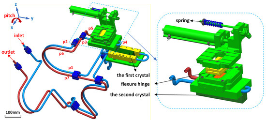
Figure 1.
DCM structure and cooling system.
The structural mesh of the DCM is illustrated in Figure 2, where the inner surface of the pipelines belongs to the fluid–solid coupling interface. Therefore, a double layer of hexahedral elements was used to discretize the pipelines. The hinges serve as the primary deformation components, with the most diminutive geometric dimensions near the axis of rotation, resulting in minimal stiffness. The reasonableness of the discretization of the hinges is crucial for the accuracy of solid domain simulations. At the axis of rotation of the hinge, this research employed four layers of hexahedral elements to capture the geometric shape more accurately. The smallest mesh size at this location is only 0.076 mm. As for the spring used to balance gravity, this research employed a more accurate solver with built-in standard spring properties without mesh partitioning. During the simulation, fixed constraints were applied to the clamping plate at the upper end of the flexible hinge and both ends of the cooling circuit for the second crystal.
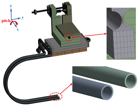
Figure 2.
Finite element model of mechanical structure.
Heat exchange in the cooling system primarily occurs in the U-shaped circuit of the first crystal, and at the inlet and outlet of the curved pipes in the second crystal circuit; fixed supports are designed for the pipes. Therefore, fluid movement has a minimal impact on crystal vibration before the fixed support of the first crystal circuit and after the fixed support of the second crystal circuit. The focus is on the region from the inlet of the U-shaped circuit for the first crystal to the outlet of the second crystal circuit. The mesh partitioning for the fluid domain is depicted in Figure 3. For the inlet mesh of the fluid, the outer layer uses hexahedral mesh elements with a height of 0.3 mm to place the fluid near the wall in the logarithmic region [7]. This facilitates solving the motion state of the fluid near the wall using the k-ε wall function method.
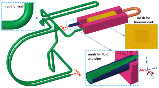
Figure 3.
Finite element model of fluid–thermal coupling. The green part is the mesh of the liquid nitrogen. The yellow part is the mesh of Si crystal (the first crystal). The pink part is the mesh of copper blocks used for cooling. The other parts are mesh of stainless-steel pipes.
In this paper, a mesh independence test is performed on the above mesh. The above mesh is Case 4 in Table 1. In the structural domain, the hinge is a critical deformation component. Through Table 1 and Figure 4, it is observed that by adjusting the mesh size of the hinge, the maximum predicted equivalent stress in Case 4 no longer undergoes significant changes under the influence of gravity. This indicates that the simulation results are independent of the mesh. In the thermal–fluid coupling analysis, the maximum temperature of the first crystal in Case 4 no longer changes. Considering both accuracy and efficiency in the calculations, this paper adopted Case 4 for numerical simulations.

Table 1.
The number of elements corresponding to each case in the mesh independence test.
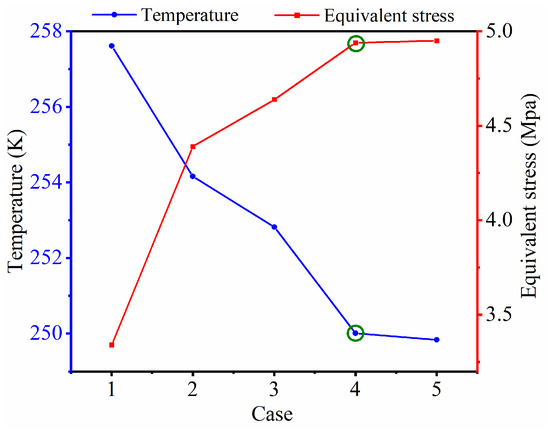
Figure 4.
The variation trends of temperature and stress in the mesh independence test. The abscissa corresponds to the 5 cases of mesh in Table 1. The blue line represents the temperature change trend, monitoring the maximum temperature on the surface of the first crystal, while the red line represents the stress change trend, monitoring the maximum equivalent stress of the flexible hinge. The green circles indicate that after this point, further mesh refinement will no longer result in significant changes in the corresponding parameters.
2.2. One-Way Fluid–Solid Coupling Numerical Simulation Method
In fluid–solid coupling calculations, the fluid domain is solved based on the mass conservation (continuity equation) and the conservation of momentum, and the solid structure is computed according to the governing equation for solid deformation.
The continuity equation is [8]:
where is the density of the cooling medium, and is the velocity vector.
The Conservation of momentum equation [9] is:
where is the density of the fluid, is the time, is the velocity vector, is the pressure, is the stress tensor, is the gravitational acceleration vector, and is the external force vector.
During the phase-change simulation, the widely employed Lee model was utilized, which is currently the most extensively applied phase-change model. The Lee model [10] of continuity equation is:
where is the volume fraction of vapor, is the vapor density, and is the velocity vector; the subscript “” is the vapor phase, is the mass transfer source term.
The equation for solving the mass transfer source term in the Lee model for the phase change process is:
where subscript “” represents the liquid phase, represents temperature, and is the saturation temperature of liquid nitrogen. is the phase change mass transfer coefficient, and subscripts “” and “” are the vaporization and condensation processes, respectively.
The governing equation for solid deformation is:
where is the density of the solid material, is the local acceleration vector, is the Cauchy stress tensor, and is the volume force tensor.
The vibration analysis in fluid–solid coupling calculations involves the equivalent of displacement and stress. Of course, in this model that includes heat transfer, it is also necessary to adhere to the principles of temperature and heat flux equivalent. At the fluid–solid coupling interface, some of the physical quantities of the fluid and the solid should act as boundary conditions for each other, namely:
where and represent the fluid side and solid side near the fluid–solid coupling interface, respectively; is displacement, is stress, is the normal stress at the fluid–solid coupling interface, is temperature, and is heat flux.
The fluid–solid coupling method can be categorized into two types: two-way fluid–solid coupling and one-way fluid–solid coupling. Two-way fluid–solid coupling is typically employed when both the fluid and structural domains undergo significant deformations, where changes in one physical domain significantly impact the geometric dimensions and shape of the other domain, particularly at the interface [11]. In the cooling system of the DCM, the deformation of the solid structure is minimal and insufficient to affect the motion characteristics of the fluid significantly. Simultaneously, the movement of the fluid has a relatively small impact on the shape of the structural domain. Therefore, during the simulation, significant changes in the meshes of both domains are not expected. A numerical simulation method using one-way fluid–solid coupling is chosen to improve computational efficiency. This better aligns with the actual conditions of the DCM cooling system and facilitates simulation analyses under various operating conditions.
2.3. The Boundary Condition Setting of the Calculation
2.3.1. Boundary Conditions of Flow Pulsation
The pressure pulsation in the cooling system originates from the pump that supplies the low-temperature coolant. In the cooling system of the DCM, commonly used pump types include centrifugal pumps and plunger pumps, both of which induce fluid pulsations in the system. The pressure pulsation caused by centrifugal pumps is related to the pump’s blades. The oscillation frequency of the fluid is equal to the product of the pumping frequency and the number of blades, and the pulsation characteristics of the fluid over time follow the changing trend of a trigonometric function [12,13]. The fluid oscillation induced by plunger pumps is related to the driving mechanism, which employs a crank-slider mechanism. When the crank angular velocity is constant, the displacement of the slider and the crank angle have a nonlinear relationship [14], causing periodic variations in the fluid pressure supplied by the pump. Therefore, this paper introduces a velocity boundary condition with a sinusoidal trend as the pulsed excitation for the cooling system. The expression for the velocity boundary condition is given by: . Here, is the instantaneous velocity at the inlet, is the average flow velocity of the cooling system, is the amplitude of velocity pulsation caused by the pump, is the pulsation frequency, and is the moment in time. The flow rate provided by the liquid nitrogen supply system during rated power operation is L/min, corresponding to a flow velocity of m/s. As shown in Table 2, when studying the influence of pulsation frequency on the stability of the DCM, the pulsating flow velocity frequency is the excitation in the low-frequency range, and is the high-frequency range (40–400 Hz nearly covers the range of flow pulsations typically induced by low-temperature liquid nitrogen pumps; for the sake of study and analysis, this range is divided into two research sections in this paper). When investigating the influence of pulsation amplitude on the stability of the DCM, the flow velocity under the rated power of the liquid nitrogen supply system is taken as the reference, and a velocity pulsation with an amplitude A (ranging from 0.1% to 1% of the average flow velocity) is chosen as the excitation. In this section, single phase simulation is used, excluding two-phase gas–liquid flow.
Table 2.
Boundary conditions of pulsation effect.
2.3.2. Boundary Conditions for Liquid Nitrogen Boiling Simulation
In addition to the fluid pulsation caused by the pump, the system will also experience vibration due to the boiling of liquid nitrogen. As the heat load generated by the first crystal is approximately W, and the boiling point of liquid nitrogen at atmospheric pressure is K, boiling of the coolant may occur. Therefore, conducting an in-depth study of the boiling phenomenon inside the cooling system is essential.
Firstly, a comprehensive steady-state fluid–thermal two-way interaction analysis is conducted to obtain temperature field data for both solid and fluid under stable conditions. As shown in Table 3, the inlet liquid nitrogen flow velocity is 0.995 m/s, and the temperature is K, representing saturated liquid nitrogen under standard conditions. The heat flux density at the beam spot is , forming a rectangular shape with dimensions of . Its geometric center is located on the meridian of the first crystal, away from the left end face of the first crystal. Next, the temperature field data at the fluid–solid interface will be extracted for use as boundary conditions in the research of liquid nitrogen boiling. To investigate the boiling of liquid nitrogen, the volume of fluid (VOF) two-phase flow method is employed to simulate the motion of liquid nitrogen and nitrogen gas [15,16]. The pump operates at a rated power with a flow rate of L/min and an operating pressure at standard atmospheric pressure. The initial temperature of liquid nitrogen inside the flow domain is K.
Table 3.
The initial boundary conditions of liquid nitrogen boiling.
The complete incompressible conservation of momentum equation was solved using the SIMPLEC method. Energy and momentum use a second-order upwind scheme, and the equation of volume fraction by the Geo-Reconstruct scheme, and turbulent kinetic energy and turbulent dissipation rate are discretized using a first-order upwind scheme. The pressure uses the PRESTO! scheme. Adaptive time steps are used with a global maximum Courant number (CFL) of 0.5 and convergence residuals are controlled below . The simulation covers a fluid time of s, with the first s dedicated to excluding the initial liquid nitrogen inside the pipes and allowing the flow field to reach a stable state under actual operating conditions. Data sampling is performed only on the flow field at s, with a sampling interval of s. During the calculation, the minimum time step is s, and the maximum time step is s. With the support of a -core GHz high-performance workstation, the fluid calculation took 70 h. The relevant physical properties of liquid nitrogen and nitrogen gas are shown in Figure 5 [17,18].
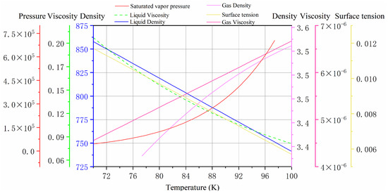
Figure 5.
Physical properties of liquid nitrogen and nitrogen.
3. Results and Discussion
3.1. Modal Analysis and Angular Calculation
The laws of vibration of an object are closely related to its intrinsic frequency. The vibration in the pitch direction of the DCM will significantly affect the quality of the beam [19]. In the DCM of SSRF, the first crystal has no freedom of motion in the pitch direction, so only the vibration in the pitch direction of the second crystal is considered. Therefore, this paper carried out a modal analysis on the overall part of the second crystal of the DCM of SSRF (including the second crystal, an angle adjustment mechanism for the second crystal, and the connected cooling piping). Figure 6 shows the results of the wet modal [20] analysis.
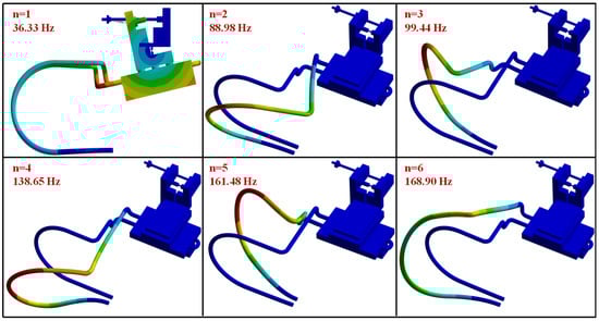
Figure 6.
Wet modal analysis of the DCM (the pressure in the pipe is generated at a liquid nitrogen flow velocity of 0.995 m/s). The color contours in the figure represent the displacement of the structure relative to the initial position, with red > yellow > green > blue. The red annotations represent the mode order and the corresponding natural frequency.
The angular displacement of the DCM is calculated based on the difference in displacement along the z direction between the two endpoints of the crystal’s meridian line, as illustrated in Figure 7. Given the small amplitude of the DCM’s vibration, the length of (in Figure 7) can be approximated as equal to the crystal’s meridian line (150 mm). Therefore, the angular displacement of the monochromator can be calculated using the following equation:
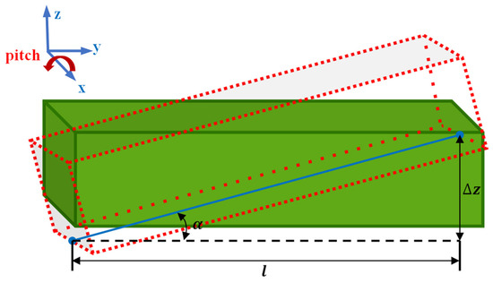
Figure 7.
Calculation of the vibration angle of the second crystal. The green portion represents the crystal’s initial position, the red dashed box represents the position of the crystal after vibration, and the blue line represents the meridian line of the crystal.
In the equation, represents the angular displacement of the DCM, rad; is the displacement difference between the two endpoints of the meridian line, mm; and l is the length of the meridian line, with = 150 mm.
3.2. Effect of Liquid Nitrogen Pulsation on DCM Stability
Figure 8 shows the pressure variation curves at seven monitoring points in the fluid domain under excitation with a frequency of 200 Hz and an amplitude of 1%∙ ( is the average flow velocity of the cooling system). From Figure 8, it can be observed that the pulsation period of pressure at each monitoring point is consistent with the excitation period, and the pulsation amplitude of pressure is more significant at the upstream monitoring points than at the downstream.
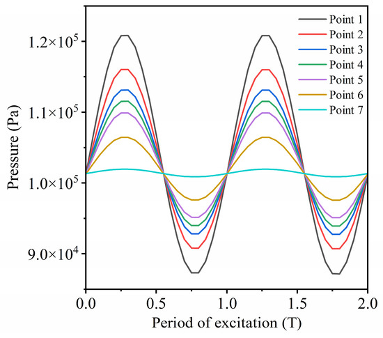
Figure 8.
Pressure changes at monitoring points. The x-axis is the time in units of pulsation periods of liquid nitrogen.
Firstly, the fluid flow must adhere to the continuity equation, which states that the total mass entering and leaving a unit fluid volume must be equal. On a macro scale, since the pipe is of constant diameter, the velocities in each section are similar. Therefore, the fluctuation in the inlet velocity will cause fluctuations in the velocities in different sections of the pipe, and the trends of these fluctuations are consistent. Next, there is energy loss in the fluid flow process, and the upstream needs to increase the pressure to maintain a smooth flow. (a) When fluid flows through the pipe, energy loss occurs due to the friction between the fluid, the pipe wall, and the internal viscosity. Energy loss is divided into along-pipe resistance loss and local resistance loss 21. The formula for calculating along-pipe resistance is given by Equation (8). (b) When the shape or size of the structural domain changes, turbulent vortices are generated in the fluid domain near the fluid–structure interface, and local relative motion intensifies. This type of motion hinders the flow of the fluid, applying backpressure locally in the opposite direction to the motion, forming back pressure. The force generated by this is called local resistance, and the calculation of local resistance uses Formula (9). Thus, the pipe resistance loss is given by: .
where represents the along-pipe resistance loss, represents the local resistance loss, is the dimensionless relative friction factor, is the length of the pipe, is the equivalent diameter of the pipe, is the density of liquid nitrogen, represents the average velocity of liquid nitrogen across the cross-section of the pipeline, and is the dimensionless local resistance coefficient, which is related to the shape and size of the pipe. The turbulent along-pipe resistance coefficient is a function of the Reynolds number and the absolute roughness of the pipe wall . When Reynolds number is constant, the friction factor is numerically positively correlated with .
Additionally, according to the energy conservation equation and the Bernoulli equation for steady flow, any two points within the fluid should adhere to:
where , and represent the pressure head, velocity head, and elevation head of the fluid per unit volume, respectively, and represents the mechanical energy loss from point 1 to point 2. The total pressure of the fluid is .
When the fluid runs stably, the pressure at the upstream monitoring point is more significant than that at the downstream. The distances between the monitoring points in the vertical direction are relatively close, with a maximum gap of only 0.1 m, and the liquid nitrogen flow velocity is 0.995 m/s. Relative to the effects of kinetic and mechanical energy losses, the influence of gravitational potential energy is negligible. Taking the monitoring points (with subscripts for upstream and for downstream) and the exit position (with subscript ) as references, the following equations follow:
due to the more significant resistance loss in the upstream pipeline than in the downstream, resulting in > , causing . However, due to flow velocity fluctuations inside the pipeline, the resistance loss is proportional to the square of the velocity, resulting in mechanical energy loss changing proportionally with the square of the velocity. When the flow velocity changes, the variation in mechanical energy loss is > . Combining Equations (11) and (12), , and consequently, the amplitude of the pressure pulsations is greater upstream than downstream.
The pressure pulsation at each point in Figure 8 does not precisely follow the trend of the excitation. Specifically, the positive pressure pulsation amplitude is more significant for each monitoring point than the negative. Taking any monitoring point as an example, when the velocity at this monitoring point changes from to , the pipeline’s resistance loss changes from to . This change can be described by Equations (13) and (14):
where is the magnitude of the velocity change. When the structure and material of the pipe do not change, the friction coefficient varies relatively. This study can ignore the change in here. From Equation (14), it can be observed that when the magnitude of velocity change is constant, the change in pipeline pressure loss is directly proportional to the initial velocity (ignoring the small numerical value of ). Therefore, when the fluid velocity is relatively large, the change in pipeline pressure loss is significant, leading to a correspondingly large change in mechanical energy loss . This results in a relatively large amplitude of pressure pulsations , consequently causing the amplitude of positive pressure pulsations to be more significant than that of negative ones.
In Figure 9, it can be observed that with the increase in the frequency of velocity pulsation, the pulsation amplitude at each point significantly increases. This is mainly due to the rapid transformation of energy in the system. The flow of liquid nitrogen in the cooling system is continuous, and the inflow and outflow are equal. When the inflow velocity decreases, the velocity at the outlet also decreases accordingly, causing the kinetic energy of the liquid nitrogen inside the pipe to transform into potential energy, acting on the internal flow field. As the frequency of velocity pulsation increases, it shortens the duration of energy conversion, reducing the kinetic energy discharged at the system outlet. More kinetic energy is stored internally, leading to a conversion into higher potential energy. This phenomenon is similar to the “water hammer effect”.
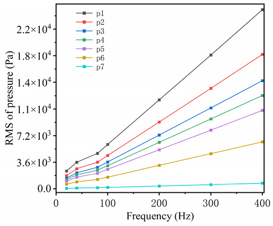
Figure 9.
Root mean square of pressure amplitude at the monitoring point.
3.2.1. Frequency Impact
Under the pulsating liquid nitrogen excitation, the vibration of the DCM is considered as forced vibration. Figure 10a and Figure 11a illustrate the time-domain curves of the DCM angular vibration under pulsating liquid nitrogen excitation. It can be observed that the crystal angular displacement exhibits harmonic response characteristics under the influence of pulsating excitation. This harmonic response is jointly induced by the structural nonlinearity within the system and the harmonic excitation generated by liquid nitrogen.
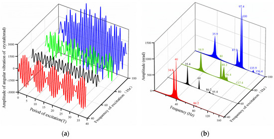
Figure 10.
The angular vibration response of the DCM under the influence of the excitation of frequency f1 (the abscissa is the time in units of pulsation periods of liquid nitrogen, and all short horizontal lines in the figure represent “minus sign”). (a) Time domain feature. (b) Frequency domain feature.
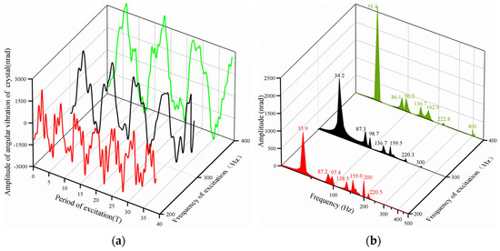
Figure 11.
The angular vibration response of the DCM under the excitation of frequency f2 (the abscissa is the time in units of pulsation periods of liquid nitrogen). (a) Time domain feature. (b) Frequency domain feature.
The internal system includes elastic elements such as flexible hinges, springs for balancing gravity, and external pipelines. Since the DCM has the minimum stiffness in the pitch direction, its vibration mainly manifests as the swinging of the crystal around the hinge center, with the trajectories of various points approximating a circular arc in the plane. Usually, the restoring force of elastic elements satisfies a proportional relationship with displacement only along the designed force line. However, this linear relationship is easily disrupted when the action point moves in space. Furthermore, the amplitude of pressure pulsation along the fluid path constantly changes, causing pulsating pressure differences at the inlet and outlet of the U-shaped pipe at the second crystal, triggering z direction vibrations of the second crystal. The vibration induces distortion in the flexible hinge. The continuously changing distortion angle causes the hinge stiffness to vary, thereby leading to changes in the elastic coefficient of the flexible hinge in the pitch direction.
Performing a Fourier transform on the time-domain curves of the crystal vibration response yields Figure 10b and Figure 11b. From these two spectra, it can be observed that the response frequency of the DCM forced vibration is composed of the natural frequency of the DCM and the coolant excitation frequency.
Considering the precision mechanical characteristics of the DCM, the amplitudes are generally small, ranging from micrometers to even nanometers. Therefore, linearizing the analysis of such ultra-low amplitude nonlinear vibrations in a specific direction is often possible. In the z direction, by converting the crystal’s displacement in the heading direction into an angle, this research can obtain the angular variation of the second crystal. The following linear harmonic excitation vibration response equation [22] exists:
is the crystal displacement at the time, is the amplification factor of the harmonic response, is the excitation amplitude, is the excitation frequency, is the phase difference of the vibration response, is the natural frequency of the structure, and is the viscous damping coefficient.
As shown in Figure 10 and Figure 11, in this forced vibration system, the pulsation frequency of the coolant will significantly excite the nearby natural frequency of the DCM. In the low-frequency range, the first natural and excitation frequencies are the DCM vibration’s master frequencies. Under high-frequency excitation, the first mode mainly dominates the DCM vibration. When the excitation frequency is 40 Hz, this frequency is close to the first mode of the structure, resulting in a significant amplification factor of the vibration, and the first mode is significantly excited. Currently, the response frequency of the DCM is the frequency of the excitation and the first mode. When the excitation frequency is 60 Hz, the DCM vibration amplitude is minimal, and this excitation frequency is almost equidistant from the first mode and the second mode frequencies. In this case, the response of the DCM is still dominated by the first mode and the excitation frequency. However, the amplitude of the first mode is lower than the operating condition at 40 Hz, since when , the amplification factor X decreases faster than ( is the amplification factor at resonance, the maximum gain of amplitude). When the excitation frequency is 80 Hz, the DCM frequency is still the first mode and the excitation frequency. This is mainly due to the significant increase in excitation amplitude caused by the increase in excitation frequency. Although the amplification factor X decreases slightly at this time, the first mode frequency remains the master vibration frequency due to increased excitation amplitude. The second mode of the system is manifested as the U-shaped pipe outlet section swinging in the z direction, with a small contribution to the DCM’s vibration in the pitch direction. In addition, at the end of the outlet pipe, the pressure pulsation amplitude is minimal. Although the amplification factor of the second mode is significant at this frequency, the peak at 88.2 Hz in the frequency amplitude diagram is not significant. When the excitation frequency is 100 Hz, it is close to the third mode frequency (99.4 Hz) of the DCM, making the system resonant. At the same time, with the increase in the amplitude of the pipeline pressure pulsation, the third mode of the DCM is significantly excited. At this time, the pipe at the entrance of the U-shaped circuit undergoes significant swinging, triggering a significant vibration of the DCM in the pitch direction.
In the high-frequency range of excitation, the first mode is the dominant manifestation of the DCM vibration response. The DCM has minor stiffness in the pitch direction, and it only exhibits rotation of the crystal around the flexible hinge in the first mode. This modal vibration contributes maximally to the DCM’s pitch-directional motion. In addition, the system’s natural frequency does not match the high-frequency excitation (200 Hz, 300 Hz, 400 Hz). With the significant increase in the excitation amplitude, the amplitude of the first mode response of the DCM gradually increases. Specifically, the increase in the excitation frequency causes a larger amplitude of the DCM response, indicating that the impact of the pressure amplitude caused by the rapid conversion of energy is stronger than the impact of the amplification factor in the high-frequency excitation region.
The above analysis shows that the DCM’s vibration response is mainly influenced by the pressure pulsation caused by the velocity pulsation of liquid nitrogen, and the pressure pulsation is also influenced by the pipeline resistance. The vibration response amplitude of the DCM is positively correlated with the amplitude of pressure pulsation. In the high-frequency range, the impact of excitation amplitude on vibration is more pronounced than the amplification factor changes caused by frequency, suggesting that the pressure amplitude variation caused by fluid frequency has a more significant impact on vibration in the high-frequency region.
In the design of the liquid nitrogen cooling system, efforts should be made to reduce pipeline resistance to lower the excitation amplitude brought by flow pulsation, for example, by polishing and grinding to reduce the roughness of the pipeline, increasing the diameter of the pipeline or reducing the length of the pipeline to decrease along-the-path resistance, increasing the curvature at pipe bends, and adopting equal or gradual diameter pipeline designs to reduce local resistance in the system.
Considering the impact of excitation frequency on system vibration, measures should be taken to reduce high-frequency excitation to ensure system stability. In addition, the operating range of the pump frequency should be positioned after the first-order frequency to reduce the amplification factor when the crystal is subjected to forced vibration. Choosing a pump with high flow and low speed is advisable. A lower speed pump causes lower pulsation frequency, and lower frequency ensures flow stability. Reciprocating pump types can be chosen, since under constant flow conditions the pulsation frequency generated by reciprocating pumps is often lower than that of centrifugal pumps.
The influence of external pipelines should be given special attention in system design. The second and third modal vibrations of the DCM are the bending vibrations of the outlet and inlet bends of the U-shaped circuit. When the system experiences second and third modal vibrations, the external pipelines generate displacement components in the z direction, causing vibration in the crystal. The natural frequency of external pipelines is relatively high, making it prone to resonance when the pump is running. Therefore, it is necessary to strengthen the rigidity of external pipelines, increase their modal frequency, and keep them away from the frequency range of flow pulsation excitation.
3.2.2. Amplitude Influence
In the experiment, this research investigated the influence of different amplitude pulsating liquid nitrogen at 200 Hz on the vibration of the DCM. The relevant results are presented in Figure 12. As the flow pulsation amplitude continuously increases, the phase angle and frequency of the DCM response remain consistent, with the only variation being a gradual enhancement of the response amplitude. According to Equations (15)–(17), when the excitation frequency is constant, the harmonic vibration response is only related to the excitation amplitude. Since the DCM’s flow velocity amplitude is positively correlated with the pressure pulsation amplitude, changes in the pulsation amplitude will not alter the trend of the DCM vibration response. They will only affect the amplitude size of the vibration.
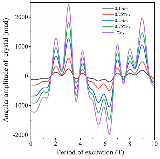
Figure 12.
The vibration response curve of the crystal under the influence of amplitude of pulsation.
In Figure 13, it is found that there is a linear relationship between the amplitude of DCM vibration and the amplitude of flow velocity pulsation. The intercept of the linear equation is 9.544, indicating that when the excitation amplitude is 0, the DCM’s vibration amplitude will attenuate to a few nanoradians. The non-zero intercept is due to errors in the simulation analysis. From Equations (8) and (15), it can be observed that when the amplitude changes of flow velocity fluctuation are small (), the pressure changes have a linear relationship with . This linear relationship is crucial for engineering practice because it validates the correctness of our linearized analysis of the nonlinear problem and provides a method for controlling and predicting system responses. In practical applications, a flow rate pulsation attenuator can be designed to reduce the vibration amplitude of the DCM.
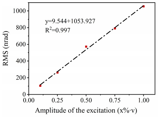
Figure 13.
The root mean square of amplitude.
3.3. Impact of Liquid Nitrogen Boiling on the Stability of the DCM
3.3.1. Temperature Field Analysis
Simulations were conducted for the DCM crystal temperature and the liquid nitrogen flow state for the pump’s rated power operation. The temperature field distribution of a crystal is shown in Figure 14a, with the lowest temperature around 80.98 K near the entrance of the cooling circuit and the highest temperature at the geometric center illuminated by the beam, approximately 249.97 K. Figure 14b illustrates the temperature field distribution on the wall of the U-shaped circuit. In this contour plot, heat is mainly concentrated in the wall area closest to the beam, gradually decreasing along the axis. In the radial direction of the pipe, the temperature distribution is nearly symmetrical.
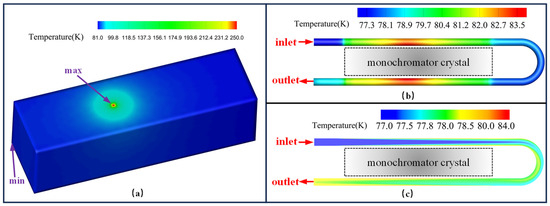
Figure 14.
Temperature distribution. (a) The first crystal. (b) The wall of the U-shaped circuit of the first crystal. (c) Liquid nitrogen in the U-shaped circuit.
Figure 14c displays the temperature field distribution inside the nitrogen circulation loop. The liquid nitrogen temperature gradually increases from the entrance to the loop exit. In the region close to the wall of the fluid, influenced by the near-wall effect and the proximity to the heat source in space, the temperature of liquid nitrogen rises more significantly. When the liquid nitrogen flows through the curved pipe, under the influence of turbulence and secondary flow, the fluid is mixed, resulting in a uniform temperature field near the exit of the curved pipe. Due to the secondary heating effect on the wall of the outlet segment, the temperature near the boundary layer reaches 84 K. At the outlet of the loop, the liquid nitrogen temperature is around 78.25 K, exceeding the saturation boiling point of liquid nitrogen at atmospheric pressure, leading to boiling.
3.3.2. Gas–Liquid Two-Phase Flow Simulation
Figure 15a illustrates the distribution of gas volume fraction in the cooling loop. Liquid nitrogen boiling begins at the inlet section of the cooling loop, forming a bubbly flow. Subsequently, during the secondary heating process in the cooling loop, the gas volume fraction gradually increases, forming slug flow [23] in the cooling loop of the first crystal.
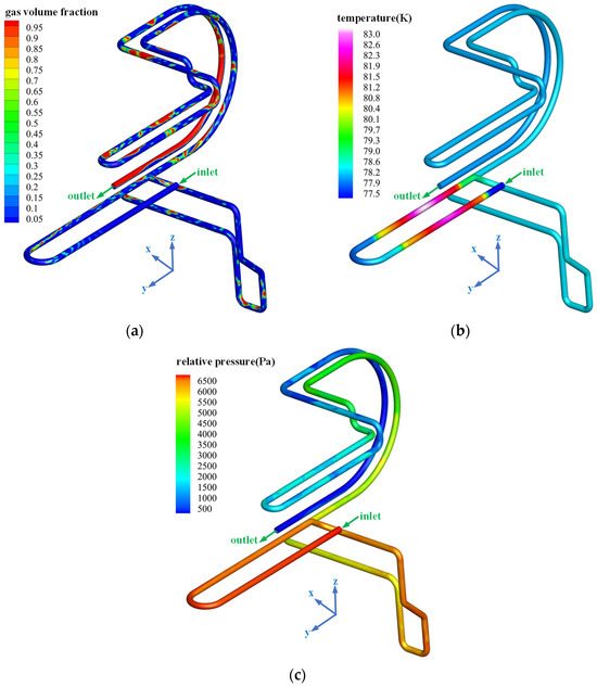
Figure 15.
Two-phase flow field cloud map. (a) Gas distribution. (b) Temperature field contour plot. (c) Relative pressure contour plot.
The development of a two-phase flow downstream in the heating loop results from the combined effects of superheated boiling and the decrease in saturation vapor pressure. The temperature cloud map of the cooling loop wall in Figure 15b shows that after liquid nitrogen flows out of the cooling loop of the first crystal, it still has a relatively high temperature, indicating that the liquid nitrogen is in a superheated state. Over time, the superheated liquid nitrogen continuously undergoes vaporization, gradually increasing the gas volume fraction downstream. The phase-change model used in this research is the Lee model, and the occurrence of boiling or condensation is related to the saturation temperature of liquid nitrogen. As shown in Figure 15c, the pressure gradually decreases with the extension of the flow path, causing the saturation temperature to drop. Therefore, gas continues to be generated inside the downstream loop.
Based on the simulation results, when the gas–liquid two-phase flow passes through the bends in the pipeline, the fluid velocity slows down, and the bubbles in the fluid merge. Bubbles near the inner side of the bend entrance momentarily pause and merge with subsequent inflowing bubbles before entering the bend. This phenomenon was also observed by Deng Dong [24] in visual experiments on liquid nitrogen flow through bends, where bubbles seemed to be momentarily “frozen”. This phenomenon occurs because the fluid behavior is complex at the bend, and there is significant local resistance at the bend entrance. The gas phase has low inertia during the flow process, and its kinetic energy is insufficient to overcome the resistance loss, leading to a rapid decrease in velocity. When it merges with subsequent bubbles into a much larger bubble, it hinders the liquid phase flow in the pipeline. Under the push of the liquid phase, the merged big bubble can then passively enter the bend. As liquid nitrogen flows to the two-crystal circuit, the gas–liquid two-phase flow in the pipeline evolves into slug flow.
Slug flow is characterized by the alternating gas and liquid flow, representing a strongly turbulent gas–liquid two-phase flow phenomenon. Due to the significant difference in fluid density between the gas and liquid phases and speed differences between the gas and liquid phases, there is a significant difference in fluid energy within a unit volume. Under the action of centrifugal force, the liquid is “thrown” to the outside of the pipe, squeezing the bubbles into the inside. The obstruction of the pipeline causes the direction of fluid motion to change continuously, leading to changes in fluid momentum. This results in the continuous impact of the alternating gas–liquid two-phase flow on the pipeline, causing the pressure field on each side of the pipeline wall to change continuously. Under the influence of centrifugal force, the pressure on the outer side of the bend wall is higher than the inner side, leading to continuous changes in pressure on both sides of the bend wall and ultimately causing pipeline instability.
As shown in Figure 15a, after the slug flow exits the bend and reaches the straight pipe, due to the influence of gravity, the gas initially on the inside of the bend rises toward the top of the pipe. This process triggers intense oscillations in the flow field. In the two-crystal circuit, there are numerous L-shaped, U-shaped, and arc-shaped pipelines, and the movement of the gas–liquid two-phase flow near these pipelines is complex, causing drastic changes in internal pressure.
3.3.3. Crystal Vibration Response
Under the influence of gas–liquid two-phase flow, the amplitude response of the DCM is shown in Figure 16. From Figure 16a, it can be observed that, compared to velocity pulsation, the impact of gas–liquid two-phase flow on the stability of the crystal is significantly enhanced. Under the effect of slug flow, the system reaches relative stability at 0.27 s, followed by resonance. Through the frequency-amplitude diagram in Figure 16b, it can be found that the fundamental frequency of the response is 35.5 Hz, which is the first-order modal frequency of the DCM vibration.
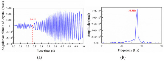
Figure 16.
The vibration response plot of the DCM under the action of gas–liquid. (a) Time domain feature. (b) Frequency domain feature two-phase flow.
Figure 17 shows the change in liquid volume fraction at the x-z section of monitoring point p3. The figure shows that the curve of liquid volume fraction in the section has significant breaks at certain moments, exhibiting a low-frequency pulse signal. The energy of the fluid is intermittent, and the fundamental frequency of the pulse excitation is very close to the first-order modal frequency of the DCM, continuously impacting the outer wall of each bend in the pipeline. After the slug flow exits the bend, under the influence of gravity, the high-energy liquid phase will fall back to the bottom of the pipe and then impact the pipeline again. Moreover, for the pulse excitation signal, the response amplitude of the DCM is related to the integration of this pulse signal segment. Hence, the vibration of the DCM induced by slug flow is higher than the influence of harmonic signals.
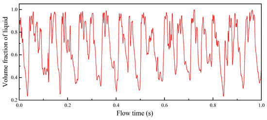
Figure 17.
Liquid volume fraction at monitoring point 3.
To avoid liquid nitrogen boiling, commonly used methods mainly include increasing the degree of undercooling, raising the flow rate, and elevating the saturation boiling point. Hossein Khosroabadi [25] and others pointed out that increasing the degree of undercooling can lead to the crystal temperature field being in the “cold expansion” range, causing the crystal surface to cave in. Taking measures to increase the flow rate imposes higher requirements on the performance indicators of pumps and pulsation attenuators. This can improve the turbulence intensity inside the pipeline, making designing an ultra-stable DCM cooling system more challenging. Kristiansen and others carried out testing at the MAX IV laboratory in Sweden and found that high-pressure conditions are favorable for minimizing DCM vibration. Their test data showed that their pipeline withstood a pressure of 5.9 standard atmospheres, raising the saturation temperature of liquid nitrogen from the standard condition of 77.36 K to around 91.89 K. This ensures that heat is wholly absorbed before liquid nitrogen boils, preventing the occurrence of gas–liquid two-phase flow-induced vibration. Additionally, it is possible to reduce local resistance in the pipeline by increasing the curvature of the cooling pipeline and shortening the distance between the boiling point and the second crystal to avoid the transition from bubbly flow to slug flow.
4. Conclusions
This article points out that the flow-induced vibration in the DCM cooling system is mainly caused by the liquid nitrogen pulsation supplied by the pump, and the oscillation and impact caused by the two-phase flow of gas and liquid. To better understand fluid-induced vibration phenomena, this paper conducted a modal analysis of the DCM, coupled numerical simulation of fluid–thermal–solid, and flow field analysis of liquid nitrogen phase transition. The temperature distribution and coolant flow state during the operation of the DCM at the Shanghai Synchrotron Radiation Source beamline were successfully simulated, and the vibration response of the crystal’s second crystal under various conditions was ultimately determined. Based on the results of numerical simulations, valuable recommendations are provided for designing and optimizing the DCM cooling system.
- The fundamental cause of the DCM vibrations induced by pulsating excitation is attributed to pipe resistance. In the design of the cooling system structure, measures can be taken to reduce pipeline resistance or flow velocity, such as choosing smooth pipes, increasing pipe diameter, reducing pipe length, and increasing the curvature of bends.
- There is a linear relationship between the amplitude of velocity pulsation and the amplitude of DCM vibration. It is necessary to design a flow pulsation attenuator to weaken the amplitude of velocity pulsation fundamentally.
- Elevating the modal frequency of the pipeline and ensuring that the excitation frequency is between the low first and second modal frequencies can reduce the amplification factors of low-order modal responses. When the frequency of the velocity pulsation is high, the pressure pulsation caused by the rapid conversion of energy has a significant impact.
- When liquid nitrogen boils under high thermal load conditions, the generated two-phase gas–liquid flow will significantly affect the system’s vibration. Adopting a high-pressure cooling system and utilizing large-radius bends in the piping is recommended to mitigate the adverse effects caused by slug flow.
Author Contributions
Conceptualization, X.G. and A.L.; methodology, A.L.; software, A.L. and K.C.; validation, X.G. and Q.L.; formal analysis, X.G.; investigation, Y.B.; resources, X.G. and Q.L.; data curation, S.L.; writing—original draft preparation, A.L. and W.Z.; writing—review and editing, X.G. and Y.B.; supervision, X.G.; project administration, X.G. and Q.L.; funding acquisition, X.G. All authors have read and agreed to the published version of the manuscript.
Funding
This research was funded by the National Natural Science Foundation of China (No. 62375261, 61974142) and National Key Research and Development Program of China (No. 2023YFA1608603).
Institutional Review Board Statement
Not applicable.
Informed Consent Statement
Not applicable.
Data Availability Statement
The original contributions presented in the study are included in the article, further inquiries can be directed to the corresponding author.
Acknowledgments
Thanks to Yuan Song, a researcher in the Beamline Equipment Research Group, for his assistance in data checking and manuscript revision for this paper.
Conflicts of Interest
The authors declare no conflicts of interest.
References
- Sergueev, I.; Döhrmann, R.; Horbach, J.; Heuer, J. Angular Vibrations of cryogenically cooled double-crystal monochromators. J. Synchrotron Radiat. 2016, 23, 1097–1103. [Google Scholar] [CrossRef] [PubMed]
- Yamazaki, H.; Shimizu, Y.; Kimura, H.; Watanabe, S.; Ono, H.; Ishikawa, T. Present status of pin-post water-cooled silicon crystals for monochromators of spring-8 X-ray undulator beamlines. AIP Conf. Proc. 2007, 879, 946–949. [Google Scholar] [CrossRef]
- Yamazaki, H.; Shimizu, Y.; Shimizu, N.; Kawamoto, M.; Kawano, Y.; Senba, Y.; Ohashi, H.; Goto, S. Present status of stability improvement of SPring-8 standard x-ray monochromators. In Proceedings of the SPIE 7077, Advances in X-ray/EUV Optics and Components III, San Diego, CA, USA, 3 September 2008; p. 707719. [Google Scholar] [CrossRef]
- Kristiansen, P.; Johansson, U.; Ursby, T.; Jensen, B. Vibrational stability of a cryocooled horizontal double-crystal monochromator. J. Synchrotron Radiat. 2016, 23, 1076–1081. [Google Scholar] [CrossRef] [PubMed]
- Fan, Y.; Li, Z.; Xu, Z.; Zhang, Q.; Liu, Y.; Wang, J. High-Precision In-Situ Detection Technology for Monochromator Crystal Angle Micro-Vibration. Chin. Opt. 2020, 13, 156–164. (In Chinese) [Google Scholar] [CrossRef]
- Qin, H.; Fan, Y.; Zhang, L.; Jin, L.; He, Y.; Zhu, W. Design and stability performance of a cradle type cryo-cooled monochromator at Shanghai Synchrotron Radiation Facility. Nucl. Instrum. Methods Phys. Res. Sect. A Accel. Spectrometers Detect. Assoc. Equip. 2022, 1027, 166350. [Google Scholar] [CrossRef]
- Granda, M.; Trojan, M.; Taler, D. CFD analysis of steam superheater operation in steady and transient state. Energy 2020, 199, 117423. [Google Scholar] [CrossRef]
- Zhang, M.; Jing, S.; Li, G. Engineering Fluid Mechanics; Xian Jiaotong University Press: Xi’an, China, 2006. (In Chinese) [Google Scholar]
- Chen, W.; Mao, Z.; Tian, W. Water cooling structure design and temperature field analysis of permanent magnet synchronous motor for underwater unmanned vehicle. Appl. Therm. Eng. 2024, 240, 122243. [Google Scholar] [CrossRef]
- Lee, W.H. Pressure Iteration Scheme for Two-Phase Flow Modeling. In Multiphase Transport: Fundamentals, Reactor Safety, Applications; World Scientific Publishing Co.: Singapore, 1980; Volume 1, pp. 407–431. [Google Scholar] [CrossRef]
- Miao, H.; Chen, Y.; Lv, L.; Wang, X.; Xu, G.; Wang, N. Analysis of Flow-Induced Vibration in Heat Exchanger Tubes Based on Bidirectional Fluid-solid coupling. Nucl. Technol. 2018, 41, 80–86. (In Chinese) [Google Scholar]
- Lu, R.; Yuan, J.; Zhu, Y. Numerical Simulation and Experimental Study of Unstable Flow Inside a Waste Heat Discharge Pump. Vib. Impact 2016, 35, 33–38. (In Chinese) [Google Scholar]
- Wang, Y.; Dai, C. Steady-State Full Three-Dimensional Numerical Simulation of Low Specific Speed Centrifugal Pump in Multiphase Flow. J. Agric. Mach. 2009, 40, 89–93. (In Chinese) [Google Scholar]
- Zhong, W.; Tang, Y.; Bu, S. Modeling of Pulsation Characteristics in a Low-Temperature Liquid Nitrogen Pump. Cryog. Eng. 2014, 6, 42–45. (In Chinese) [Google Scholar]
- Liu, X.; Su, G.; Yao, Z.; Yan, Z.; Yu, Y. Numerical Study of Flow Boiling of ADN-Based Liquid Propellant in a Capillary. Materials 2023, 16, 1858. [Google Scholar] [CrossRef] [PubMed]
- Lv, B.; Xu, D.; Wang, W.; Shi, Y.; Xin, J.; Fang, Z.; Li, L. Numerical Simulation of Pulsating Two-Phase Flow in a Single-Circuit Liquid Helium Pulsating Heat Pipe. Low Temp. Eng. 2023, 1, 26–30+49. (In Chinese) [Google Scholar]
- Fu, Y.; Gao, B.; Ni, D.; Zhang, W.; Fu, Y. Study on the Influence of Thermodynamic Effects on the Characteristics of Liquid Nitrogen Cavitating Flow around Hydrofoils. Symmetry 2023, 15, 1946. [Google Scholar] [CrossRef]
- Fan, H.; Diao, Y. Fluid Mechanics; Machinery Industry Press: Beijing, China, 2020. (In Chinese) [Google Scholar]
- Liu, G.; Ma, L.; Liu, J. Handbook of Chemical and Chemical Engineering Properties; Chemical Industry Press: Beijing, China, 2002. (In Chinese) [Google Scholar]
- Duan, J.; Li, C.; Jin, J. Modal Analysis of Tubing Considering the Effect of Fluid–Structure Interaction. Energies 2022, 15, 670. [Google Scholar] [CrossRef]
- Geraldes, R.R.; Caliari, R.; Moreno, G.B.Z.L.; Ruijl, T.; Sanfelici, L.; Saveri Silva, M.; Neto, N.M.S.; Tolentino, H.C.N.; Westfahl, H., Jr. The New High Dynamics DCM for Sirius. In Proceedings of the MEDSI’16, Barcelona, Spain, 11–16 September 2016; pp. 141–146. [Google Scholar] [CrossRef]
- Cheng, Y.D. Structural Vibration Analysis; Jilin University Press: Changchun, China, 2008. (In Chinese) [Google Scholar]
- Wang, L.; Zhang, Y.; Bao, Y.; Ma, T. Numerical study of transient flow characteristics of gas-liquid two-phase flow in inclined upward tube under periodic vibration. Ocean Eng. 2023, 282, 115024. [Google Scholar] [CrossRef]
- Deng, D. Study on the Influence of Rotating Bend on the Flow and Heat Transfer of Liquid Nitrogen in a Vertical U-shaped Tube. Ph.D. Thesis, Shanghai Jiao Tong University, Shanghai, China, 2014. (In Chinese). [Google Scholar]
- Khosroabadi, H.; Alianelli, L.; Porter, D.G.; Collins, S.; Sawhney, K. Cryo-cooled silicon crystal monochromators: A study of power load, temperature and deformation. J. Synchrotron Rad. 2022, 29, 377–385. [Google Scholar] [CrossRef] [PubMed]
Disclaimer/Publisher’s Note: The statements, opinions and data contained in all publications are solely those of the individual author(s) and contributor(s) and not of MDPI and/or the editor(s). MDPI and/or the editor(s) disclaim responsibility for any injury to people or property resulting from any ideas, methods, instructions or products referred to in the content. |
© 2024 by the authors. Licensee MDPI, Basel, Switzerland. This article is an open access article distributed under the terms and conditions of the Creative Commons Attribution (CC BY) license (https://creativecommons.org/licenses/by/4.0/).