
Sample-Based Gradient Edge and Angular Prediction for VVC Lossless Intra-Coding


Abstract
1. Introduction
2. Related Works
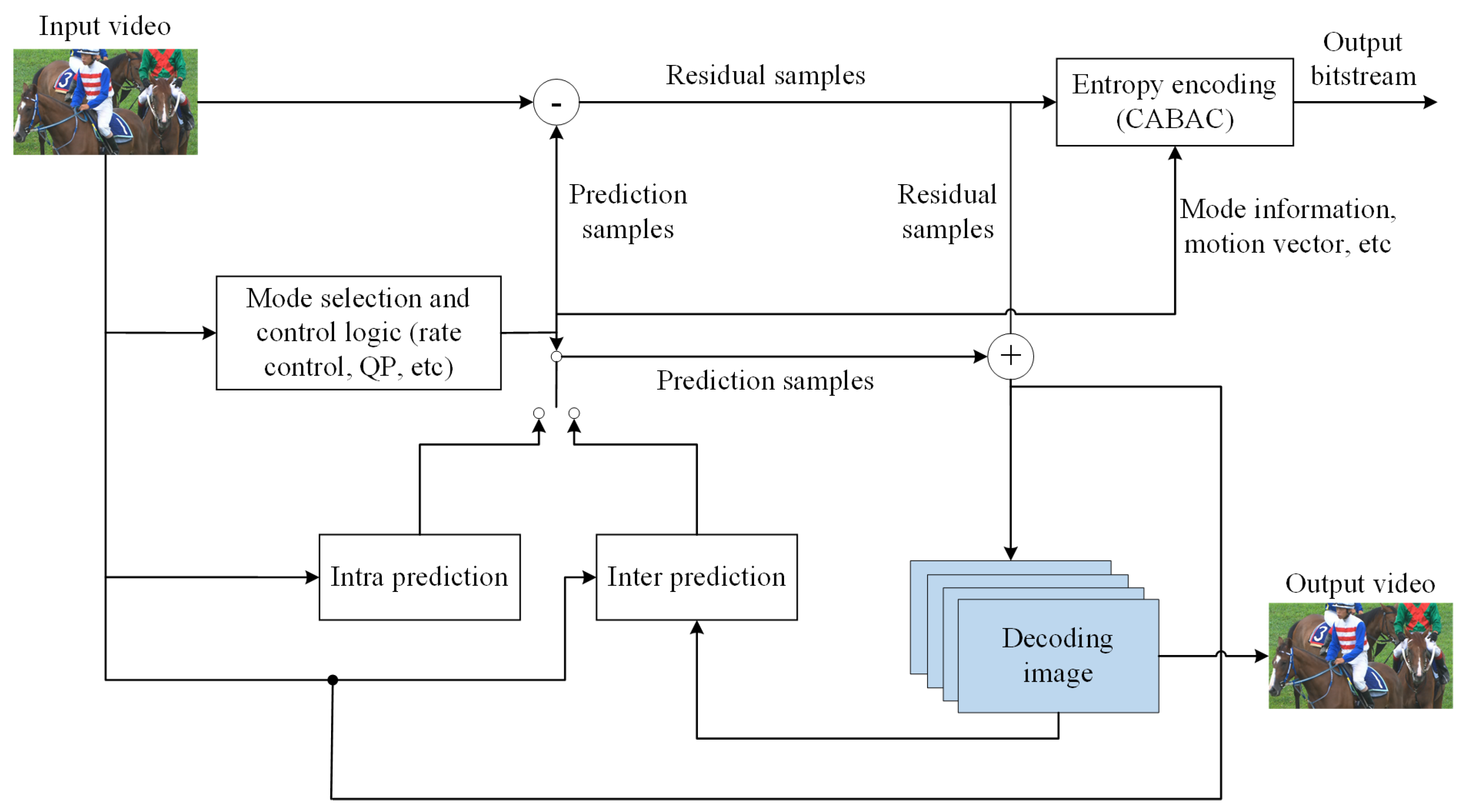
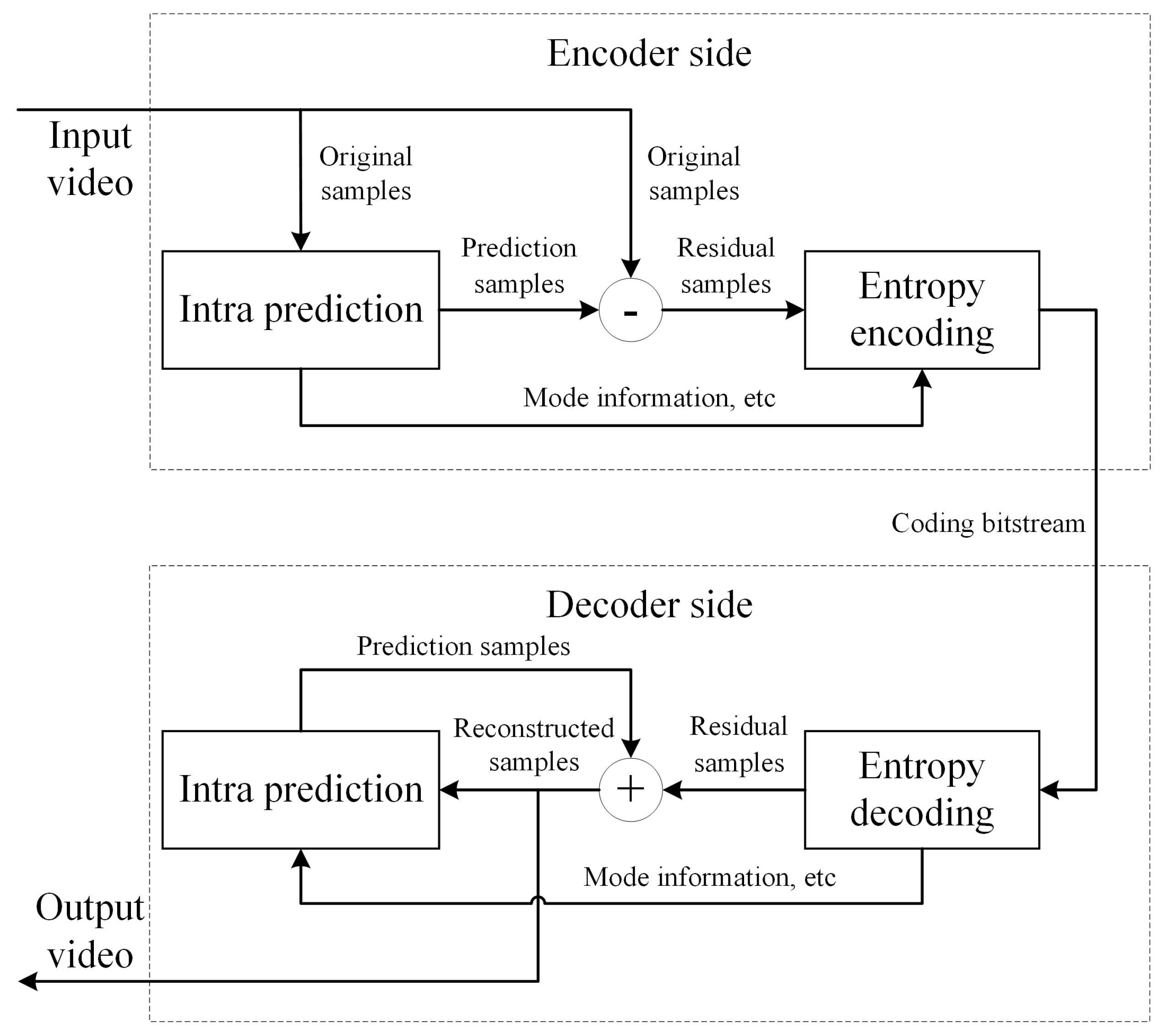
3. Proposed Method
3.1. Sample-Based Intra-Gradient Edge Detection and Angular Prediction
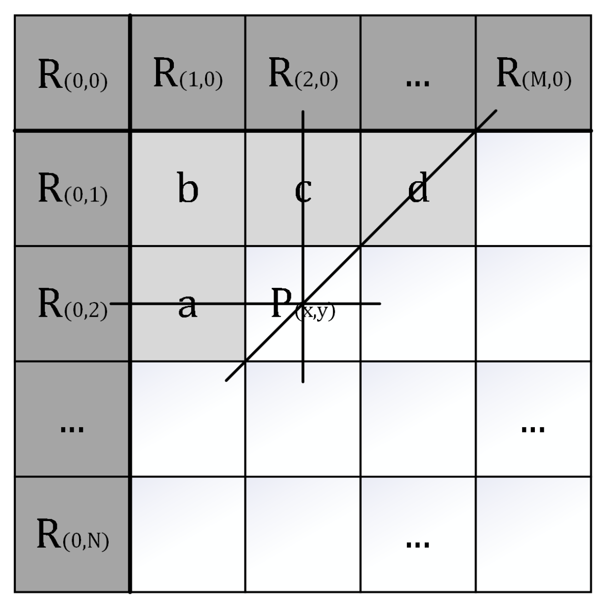
3.1.1. Edge Regions: Gradient Edge Detection
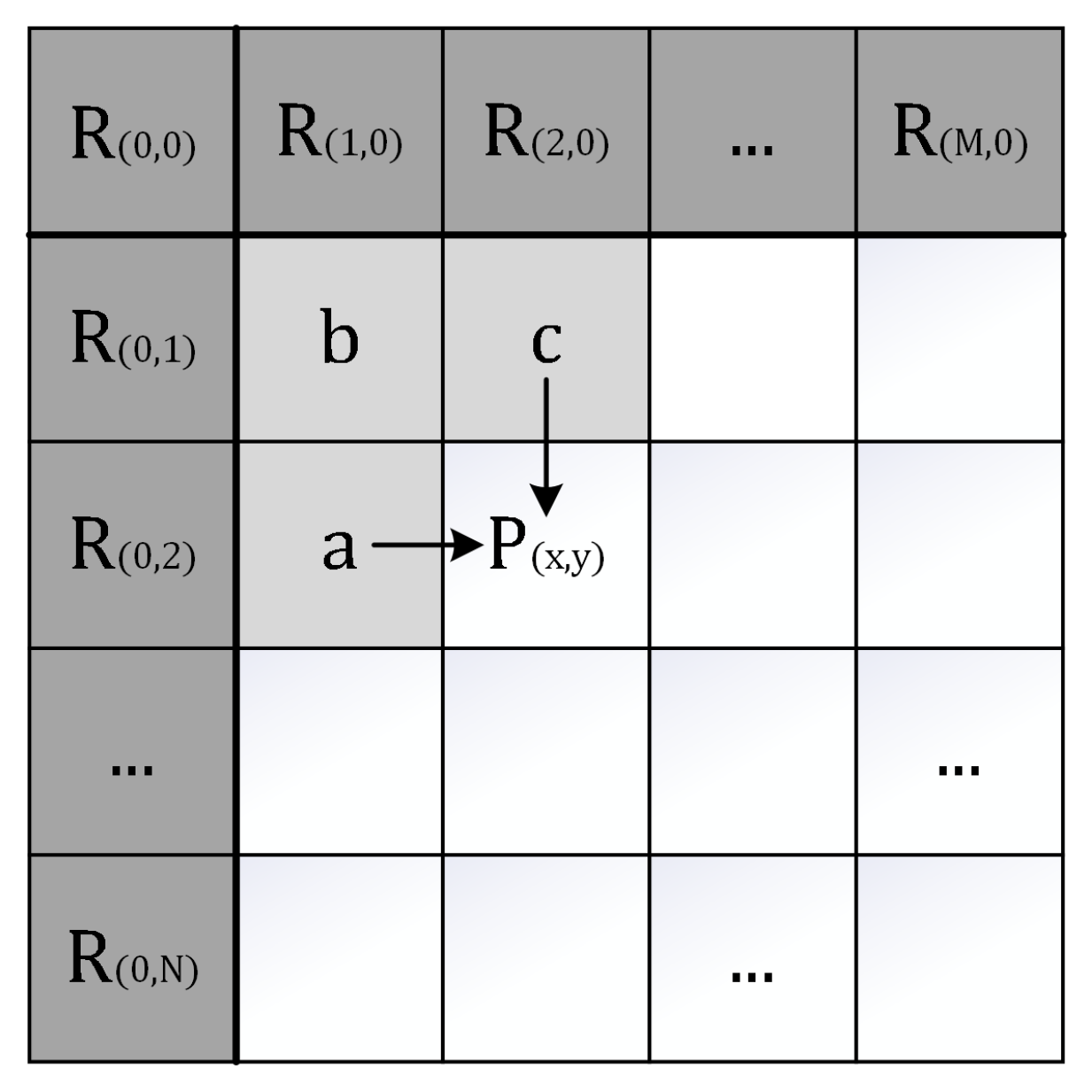
3.1.2. Smooth Regions: Average Prediction
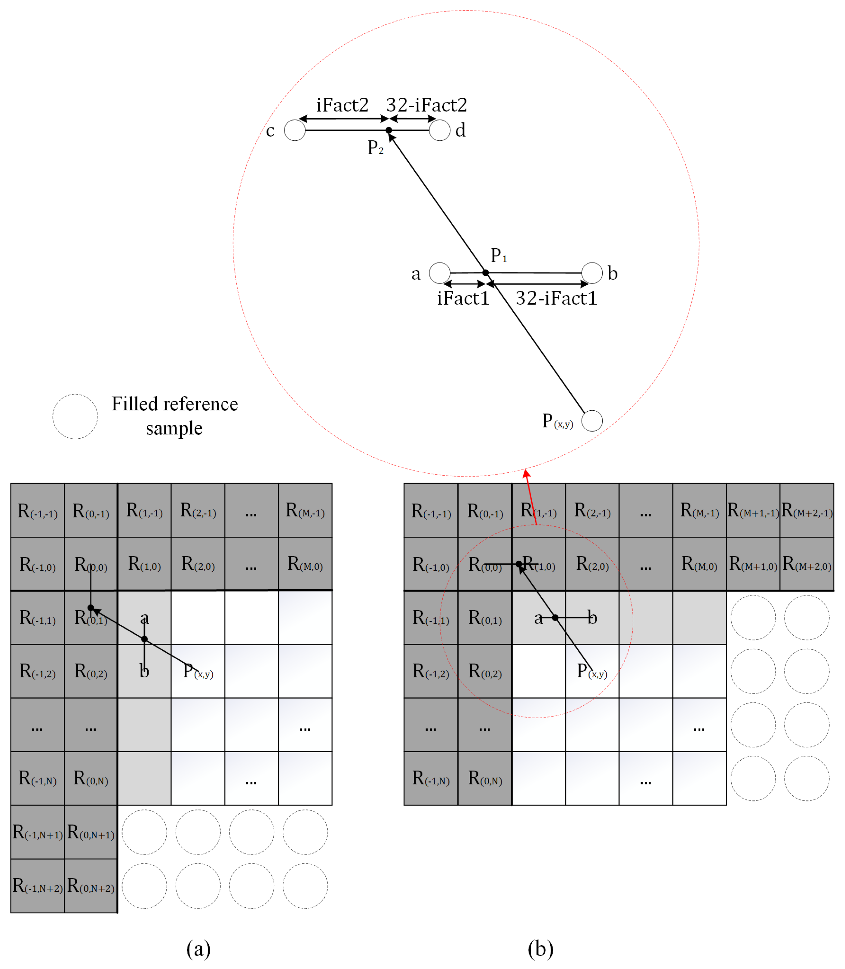
3.1.3. Directional Texture Regions: Angular Prediction
3.2. Intra-Prediction Flowchart
4. Results and Analysis
5. Conclusions
Author Contributions
Funding
Institutional Review Board Statement
Informed Consent Statement
Data Availability Statement
Conflicts of Interest
References
- Bross, B.; Wang, Y.-K.; Ye, Y.; Liu, S.; Chen, J.; Sullivan, G.J.; Ohm, J.-R. Overview of the versatile video coding (VVC) standard and its applications. IEEE Trans. Circuits Syst. Video Technol. 2021, 31, 3736–3764. [Google Scholar] [CrossRef]
- Sullivan, G.J.; Ohm, J.-R.; Han, W.-J.; Wiegand, T. Overview of the high efficiency video coding (HEVC) standard. IEEE Trans. Circuits Syst. Video Technol. 2012, 22, 1649–1668. [Google Scholar] [CrossRef]
- Wiegand, T.; Sullivan, G.J.; Bjontegaard, G.; Luthra, A. Overview of the H.264/AVC video coding standard. IEEE Trans. Circuits Syst. Video Technol. 2003, 13, 560–576. [Google Scholar] [CrossRef]
- Unno, K.; Kameda, Y.; Kita, Y.; Matsuda, I.; Itoh, S.; Kawamura, K. Lossless video coding based on probability model optimization with improved adaptive prediction. In Proceedings of the 2021 IEEE International Conference on Image Processing (ICIP), Anchorage, AK, USA, 19–22 September 2021; pp. 2044–2048. [Google Scholar]
- Zhao, L.; An, J.; Ma, S.; Zhao, D.; Fan, X. Improved intra transform skip mode in HEVC. In Proceedings of the 2013 IEEE International Conference on Image Processing (ICIP), Melbourne, Australia, 15–18 September 2013; pp. 2010–2014. [Google Scholar]
- Abdoli, M.; Henry, F.; Brault, P.; Dufaux, F.; Duhamel, P.; Philippe, P. Intra block-DPCM with layer separation of screen content in VVC. In Proceedings of the 2019 IEEE International Conference on Image Processing (ICIP), Taipei, Taiwan, 22–25 September 2019; pp. 3162–3166. [Google Scholar]
- Lee, Y.L.; Han, K.H.; Lim, S.C. Lossless intra coding for improved 4: 4: 4 coding in H. 264/MPEG-4 AVC. Joint Video Team (JVT). IEEE Trans. Image Process. 2005. [Google Scholar]
- Lee, Y.-L.; Han, K.-H.; Sullivan, G.J. Improved lossless intra coding for H.264/MPEG-4 AVC. IEEE Trans. Image Process. 2006, 15, 2610–2615. [Google Scholar] [CrossRef] [PubMed]
- Song, L.; Luo, Z.; Xiong, C. Improving lossless intra coding of H.264/AVC by pixel-wise spatial interleave prediction. IEEE Trans. Circuits Syst. Video Technol. 2011, 21, 1924–1928. [Google Scholar] [CrossRef]
- Wang, L.-L.; Siu, W.-C. Improved lossless coding algorithm in H.264/AVC based on hierarchical intra prediction. In Proceedings of the 2011 18th IEEE International Conference on Image Processing (ICIP), Brussels, Belgium, 11–14 September 2011; pp. 2009–2012. [Google Scholar]
- Lee, S.; Kim, I.K.; Kim, C. RCE2: Test 1 Residual DPCM for HEVC lossless Coding; Doc. JCTVC-M0079; Joint Collaborative Team on Video Coding (JCT-VC): Geneva, Switzerland, 2013. [Google Scholar]
- Xu, J.; Joshi, R.; Cohen, R.A. Overview of the emerging HEVC screen content coding extension. IEEE Trans. Circuits Syst. Video Technol. 2016, 26, 50–62. [Google Scholar] [CrossRef]
- Hong, S.-W.; Kwak, J.-H.; Lee, Y.-L. Cross residual transform for lossless intra-coding for HEVC. Signal Process. Image Commun. 2013, 28, 1335–1341. [Google Scholar] [CrossRef]
- Jeon, G.; Kim, K.; Jeong, J. Improved residual DPCM for HEVC lossless coding. In Proceedings of the 2014 27th SIBGRAPI Conference on Graphics, Patterns and Images, Rio de Janeiro, Brazil, 27–30 August 2014; pp. 95–102. [Google Scholar]
- Kim, K.; Jeon, G.; Jeong, J. Improvement of implicit residual DPCM for HEVC. In Proceedings of the 2014 Tenth International Conference on Signal-Image Technology and Internet-Based Systems, Marrakech, Morocco, 23–27 November 2014; pp. 652–658. [Google Scholar]
- Nguyen, T.; Xu, X.; Henry, F.; Liao, R.L.; Sarwer, M.G.; Karczewicz, M.; Chao, Y.H.; Xu, J.; Liu, S.; Marpe, D.; et al. Overview of the screen content support in VVC: Applications, coding tools, and performance. IEEE Trans. Circuits Syst. Video Technol. 2021, 31, 3801–3817. [Google Scholar] [CrossRef]
- Zhou, M.; Gao, W.; Jiang, M.; Yu, H. HEVC lossless coding and improvements. IEEE Trans. Circuits Syst. Video Technol. 2012, 22, 1839–1843. [Google Scholar] [CrossRef]
- Zhou, M.; Budagavi, M. RCE2: Experimental Results on Test 3 and Test 4; Doc. JCTVC-M0056; Joint Collaborative Team on Video Coding (JCT-VC): Geneva, Switzerland, 2013. [Google Scholar]
- Sanchez, V.; Bartrina-Rapesta, J. Lossless compression of medical images based on HEVC intra coding. In Proceedings of the 2014 IEEE International Conference on Acoustics, Speech and Signal Processing (ICASSP), Florence, Italy, 4–9 May 2014; pp. 6622–6626. [Google Scholar]
- Sanchez, V.; Aulí-Llinàs, F.; Bartrina-Rapesta, J.; Serra-Sagristà, J. HEVC-based lossless compression of whole slide pathology images. In Proceedings of the 2014 IEEE Global Conference on Signal and Information Processing (GlobalSIP), Atlanta, GA, USA, 3–5 December 2014; pp. 297–301. [Google Scholar]
- Sanchez, V. Lossless screen content coding in HEVC based on sample-wise median and edge prediction. In Proceedings of the 2015 IEEE International Conference on Image Processing (ICIP), Quebec City, QC, Canada, 27–30 September 2015; pp. 4604–4608. [Google Scholar]
- Sanchez, V.; Aulí-Llinàs, F.; Serra-Sagristà, J. Piecewise mapping in HEVC lossless intra-prediction coding. IEEE Trans. Image Process. 2016, 25, 4004–4017. [Google Scholar] [CrossRef] [PubMed]
- Weinberger, M.J.; Seroussi, G.; Sapiro, G. The LOCO-I lossless image compression algorithm: Principles and standardization into JPEG-LS. IEEE Trans. Image Process. 2000, 9, 1309–1324. [Google Scholar] [CrossRef] [PubMed]
- Sanchez, V. Sample-based edge prediction based on gradients for lossless screen content coding in HEVC. In Proceedings of the 2015 Picture Coding Symposium (PCS), Cairns, Australia, 31 May–3 June 2015; pp. 134–138. [Google Scholar]
- Sanchez, V.; Hernandez-Cabronero, M.; Auli-Llinàs, F.; Serra-Sagristà, J. Fast lossless compression of whole slide pathology images using HEVC intra-prediction. In Proceedings of the 2016 IEEE International Conference on Acoustics, Speech and Signal Processing (ICASSP), Shanghai, China, 20–25 March 2016; pp. 1456–1460. [Google Scholar]
- Wige, E.; Yammine, G.; Amon, P.; Hutter, A.; Kaup, A. Pixel-based averaging predictor for HEVC lossless coding. In Proceedings of the 2013 IEEE International Conference on Image Processing (ICIP), Melbourne, VIC, Australia, 15–18 September 2013; pp. 1806–1810. [Google Scholar]
- Wige, E.; Yammine, G.; Amon, P.; Hutter, A.; Kaup, A. Sample-based weighted prediction with directional template matching for HEVC lossless coding. In Proceedings of the 2013 Picture Coding Symposium (PCS), San Jose, CA, USA, 8–11 December 2013; pp. 305–308. [Google Scholar]
- Sanchez, V.; Aulí-Llinàs, F.; Serra-Sagristà, J. DPCM-based edge prediction for lossless screen content coding in HEVC. IEEE J. Emerg. Sel. Top. Circuits Syst. 2016, 6, 497–507. [Google Scholar] [CrossRef]
- Weng, X.; Lin, M.; Lin, Q.; Chen, G. L-shape-based iterative prediction and residual median edge detection (LIP-RMED) algorithm for VVC intra-frame lossless compression. IEEE Signal Process. Lett. 2022, 29, 1227–1231. [Google Scholar] [CrossRef]
- Chen, F.; Zhang, J.; Li, H. Hybrid transform for HEVC-based lossless coding. In Proceedings of the 2014 IEEE International Symposium on Circuits and Systems (ISCAS), Melbourne, Australia, 1–5 June 2014; pp. 550–553. [Google Scholar]
- Cai, X.; Gu, Q. Improved HEVC lossless compression using two-stage coding with sub-frame level optimal quantization values. In Proceedings of the 2014 IEEE International Conference on Image Processing (ICIP), Paris, France, 27–30 October 2014; pp. 5651–5655. [Google Scholar]
- Kamisli, F. Lossless image and intra-frame compression with integer-to-integer DST. IEEE Trans. Circuits Syst. Video Technol. 2019, 29, 502–516. [Google Scholar] [CrossRef]
- Bossen, F.; Boyce, J.; Li, X.; Seregin, V.; Sühring, K. JVET Common Test Conditions and Software Reference Configurations for SDR Video; Doc. JVET-N1010; Joint Video Experts Team (JVET): Geneva, Switzerland, 2019. [Google Scholar]


| Class | Sequence | Resolution | Frames | Frame-Rate/fps |
|---|---|---|---|---|
| A1 | Tango2 | 3840 × 2160 | 294 | 60 |
| FoodMarket4 | 3840 × 2160 | 300 | 60 | |
| Campfire | 3840 × 2160 | 300 | 30 | |
| A2 | CatRobot | 3840 × 2160 | 300 | 60 |
| DaylightRoad2 | 3840 × 2160 | 300 | 60 | |
| ParkRunning3 | 3840 × 2160 | 300 | 50 | |
| B | MarketPlace | 1920 × 1080 | 600 | 60 |
| RitualDance | 1920 × 1080 | 600 | 60 | |
| Cactus | 1920 × 1080 | 500 | 50 | |
| BasketballDrive | 1920 × 1080 | 500 | 50 | |
| BQTerrace | 1920 × 1080 | 600 | 60 | |
| C | BasketballDrill | 832 × 480 | 500 | 50 |
| BQMall | 832 × 480 | 600 | 60 | |
| PartyScene | 832 × 480 | 500 | 50 | |
| RaceHorses | 832 × 480 | 300 | 30 | |
| D | BasketballPass | 416 × 240 | 500 | 50 |
| BlowingBubbles | 416 × 240 | 500 | 50 | |
| BQSquare | 416 × 240 | 600 | 60 | |
| RaceHorses | 416 × 240 | 300 | 30 | |
| E | FourPeople | 1280 × 720 | 600 | 60 |
| Johnny | 1280 × 720 | 600 | 60 | |
| KristenAndSara | 1280 × 720 | 600 | 60 | |
| F | BasketballDrillText | 832 × 480 | 500 | 50 |
| ChinaSpeed | 1024 × 768 | 500 | 30 | |
| SlideEditing | 1280 × 720 | 300 | 30 | |
| SlideShow | 1280 × 720 | 500 | 20 |
| Class | Sequence | BDPCM | SAP | SAP1 | SAP−E | LIP−RMED | SGAP |
|---|---|---|---|---|---|---|---|
| A1 | Tango2 | −1.12 | −1.49 | −1.50 | −3.40 | −2.80 | −3.54 |
| FoodMarket4 | −3.71 | −4.76 | −4.78 | −8.76 | −7.72 | −9.37 | |
| Campfire | −0.44 | −0.43 | −0.43 | −0.54 | −0.95 | −0.78 | |
| A2 | CatRobot | −0.73 | −1.28 | −1.28 | −2.14 | −1.52 | −2.47 |
| DaylightRoad2 | −0.94 | −1.24 | −1.24 | −2.24 | −1.63 | −2.53 | |
| ParkRunning3 | −4.03 | −6.01 | −6.03 | −9.91 | −9.36 | −11.59 | |
| B | MarketPlace | −2.95 | −4.06 | −4.07 | −6.98 | −5.64 | −7.58 |
| RitualDance | −3.70 | −5.55 | −5.56 | −7.55 | −5.96 | −8.72 | |
| Cactus | −1.17 | −1.68 | −1.68 | −2.43 | −1.98 | −2.74 | |
| BasketballDrive | −1.51 | −1.71 | −1.72 | −2.15 | −2.00 | −2.75 | |
| BQTerrace | −1.70 | −1.71 | −1.71 | −2.34 | −2.56 | −2.85 | |
| C | BasketballDrill | −1.11 | −3.86 | −3.86 | −4.18 | −2.27 | −5.05 |
| BQMall | −3.09 | −3.71 | −3.72 | −4.73 | −3.53 | −5.36 | |
| PartyScene | −2.60 | −3.40 | −3.40 | −4.36 | −2.77 | −4.70 | |
| RaceHorses | −3.10 | −4.36 | − 4.37 | −7.43 | −5.65 | −7.93 | |
| D | BasketballPass | −8.01 | −9.45 | −9.45 | −12.04 | −8.70 | −13.08 |
| BlowingBubbles | −2.90 | −4.89 | −4.89 | −5.60 | −2.97 | −5.95 | |
| BQSquare | −2.01 | −2.49 | −2.49 | −3.18 | −2.31 | −3.57 | |
| RaceHorses | −4.39 | −6.56 | −6.56 | −9.58 | −7.13 | −10.47 | |
| E | FourPeople | −6.29 | −7.52 | −7.52 | −10.28 | −8.09 | −11.20 |
| Johnny | −4.92 | −6.31 | −6.31 | −8.10 | −6.22 | −8.81 | |
| KristenAndSara | −5.64 | −6.86 | −6.85 | −8.80 | −6.58 | −9.56 | |
| F | BasketballDrillText | −1.93 | −4.48 | −4.48 | −4.92 | −2.78 | −5.72 |
| ChinaSpeed | −11.42 | −12.47 | −12.48 | −13.93 | −9.22 | −15.03 | |
| SlideEditing | −10.47 | −8.26 | −8.28 | −10.05 | −9.88 | −10.89 | |
| SlideShow | −11.09 | −11.24 | −11.26 | −16.42 | −13.67 | −17.82 | |
| Average of bit−rate | −3.88 | −4.84 | −4.84 | −6.62 | −5.15 | −7.31 | |
| Scheme | Encoding Time | Decoding Time |
|---|---|---|
| BDPCM | 124.1 | 94.6 |
| SAP | 98.9 | 75.0 |
| SAP1 | 98.3 | 74.8 |
| SAP-E | 97.4 | 71.4 |
| LIP-RMED | 131.2 | 92.7 |
| SGAP | 105.4 | 74.2 |
Disclaimer/Publisher’s Note: The statements, opinions and data contained in all publications are solely those of the individual author(s) and contributor(s) and not of MDPI and/or the editor(s). MDPI and/or the editor(s) disclaim responsibility for any injury to people or property resulting from any ideas, methods, instructions or products referred to in the content. |
© 2024 by the authors. Licensee MDPI, Basel, Switzerland. This article is an open access article distributed under the terms and conditions of the Creative Commons Attribution (CC BY) license (https://creativecommons.org/licenses/by/4.0/).
Share and Cite
Chen, G.; Lin, M. Sample-Based Gradient Edge and Angular Prediction for VVC Lossless Intra-Coding. Appl. Sci. 2024, 14, 1653. https://doi.org/10.3390/app14041653
Chen G, Lin M. Sample-Based Gradient Edge and Angular Prediction for VVC Lossless Intra-Coding. Applied Sciences. 2024; 14(4):1653. https://doi.org/10.3390/app14041653
Chicago/Turabian StyleChen, Guojie, and Min Lin. 2024. "Sample-Based Gradient Edge and Angular Prediction for VVC Lossless Intra-Coding" Applied Sciences 14, no. 4: 1653. https://doi.org/10.3390/app14041653
APA StyleChen, G., & Lin, M. (2024). Sample-Based Gradient Edge and Angular Prediction for VVC Lossless Intra-Coding. Applied Sciences, 14(4), 1653. https://doi.org/10.3390/app14041653