Flame Combustion State Detection Method of Cement Rotary Furnace Based on Improved RE-DDPM and DAF-FasterNet

Abstract

It is of great significance to effectively identify the flame-burning state of cement rotary kilns to optimize the calcination process and ensure the quality of cement. However, high-temperature and smoke-filled environments bring about difficulties with respect to accurate feature extraction and data acquisition. To address these challenges, this paper proposes a novel approach. First, an improved denoising diffusion probability model (RE-DDPM) is proposed. By applying a mask to the burning area and mixing it with the actual image in the denoising process, local diversity generation in the image was realized, and the problem of limited and uneven data was solved. Secondly, this article proposes the DAF-FasterNet model, which incorporates a deformable attention mechanism (DAS) and replaces the ReLU activation function with FReLU so that it can better focus on key flame features and extract finer spatial details. The RE-DDPM method exhibits faster convergence and lower FID scores, indicating that the generated images are more realistic. DAF-FasterNet achieves 98.9% training accuracy, 98.1% test accuracy, and a 22.3 ms delay, making it superior to existing methods in flame state recognition.

1. Introduction

Recognition of the combustion state of the flame in the cement rotary kilns refers to the process of analyzing and identifying real-time images of the flame during the clinker calcination process, ensuring the smooth progress of cement production through the recognition, detection, and control of the combustion state. A flame combustion state recognition method based on a rotary kiln can provide many advantages in the cement production process. Such a method is conducive to real-time monitoring of the firing process, ensuring that workers detect abnormal conditions and take necessary measures to ensure the safety and stability of the production process. Analyzing the color, shape, and other characteristics of the flame is beneficial for detecting and evaluating the quality of cement and taking measures to improve the quality of cement production. Flame combustion images help understand the combustion efficiency, and adjusting the supply of oxygen and raw materials based on image analysis can improve production efficiency, reduce production costs, and decrease carbon emissions. However, due to complex factors such as high temperature, high pressure, and high levels of smoke inside the rotary kiln, workers’ inaccurate recognition of the combustion state can affect the effective control of the calcination process. Existing machine learning-based flame combustion state recognition methods have low accuracy and poor generalization ability due to the influence of the complex environment inside the furnace. Furthermore, deep learning-based flame combustion state recognition methods face difficulties in modeling due to low data volume and severely uneven sample distributions. Therefore, this paper proposes a new method for recognizing the combustion state of cement rotary kilns that can accurately and quickly identify the flame combustion state, even with a small and unevenly distributed data volume.

2. Related Worked

Detection and recognition methods for the clinker calcination process are mainly divided into four categories: manual observation methods, contact detection methods, infrared detection methods, and flame image processing and recognition detection methods. Manual observation methods are easily influenced by workers’ experience and lead to incorrect judgments in complex furnace environments. Contact detection methods and infrared measurement methods cannot meet the requirements of long-term continuous and real-time detection in environments with high temperature, high levels of smoke, and strong physical and chemical reactions. Most contact detection equipment requires regular maintenance and updates, consuming considerable material and human resources. Flame image processing and recognition detection methods have made great progress in recent years and cane mainly be divided into two mainstream methods: machine learning recognition methods based on manual feature extraction and deep learning recognition methods based on automatic feature extraction.

Feature-based machine learning recognition methods mainly consist of two steps: feature extraction and state prediction. The purpose of feature extraction is to convert high-dimensional data into low-dimensional feature data, which serve as input for machine learning. Wang et al. [1] proposed a method for identifying the combustion conditions of rotary kilns based on the extraction of texture features of flame images using the Gray-Level Co-occurrence Matrix (GLCM) and the KPCA-GLVQ recognition method. Zhou et al. [2] established a fuzzy support vector machine model to predict the end point of converter blowing based on flame spectral features and furnace flame characteristics. Liu et al. [3] proposed a quaternion directional statistical algorithm to extract color texture features of images, then analyzed the features using K-nearest neighbor regression and a Generalized Regression Neural Network (GRNN). Zhao et al. [4] extracted and analyzed the features of furnace flame chroma, boundary, and texture, using them as inputs. They established a model of the relationship between furnace flame images and blowing data using a least squares support vector machine network model and used the particle swarm optimization algorithm to establish the optimal prediction model, achieving good prediction results. Li et al. [5] proposed a method to describe the dynamic deformation characteristics of flames and determine the end point of steel making based on dynamic information on flame boundaries.

Flame combustion exhibits various characteristics, and the choice of which features to extract as inputs for machine learning is influenced by scholars’ “expert experience”. Different choices of features have a significant impacts on the recognition results, and such methods are difficult to generalize. Because different factories have different production scenarios, the characteristics of flame combustion vary. Moreover, the complex and changing environment inside the furnace makes it difficult for methods based on single-feature extraction to be stable. In recent years, many scholars have chosen deep learning methods that can automatically extract various features of flames for research. Yang et al. [6] proposed a novel neural network architecture that can effectively capture the spatiotemporal changes of image sequences by using a series of flame image sequences to predict the combustion state. This method can quickly and effectively predict the combustion state of rotary kilns. Sun et al. [7] proposed an improved method for determining the end point of converter blowing based on DenseNet, effectively improving the accuracy of converter end-point determination. Hu et al. [8] improved the attention loss function of the network based on DenseNet, proposed the EL-DenseNet combustion state recognition method, and further improved the recognition accuracy. Gu et al. [9] proposed a new recognition model, which first preprocesses the furnace flame video sequence, then uses a Convolutional Recurrent Neural Network (CRNN) to further learn the spatiotemporal features of the flame to obtain the recognition results. Wang et al. [10] used the bidirectional recurrent multi-scale convolutional deep neural network algorithm to take into account the characteristics of the frequency-domain structure and the time-domain dynamic sequence. It was applied to the deep learning of BOF flame spectral information.

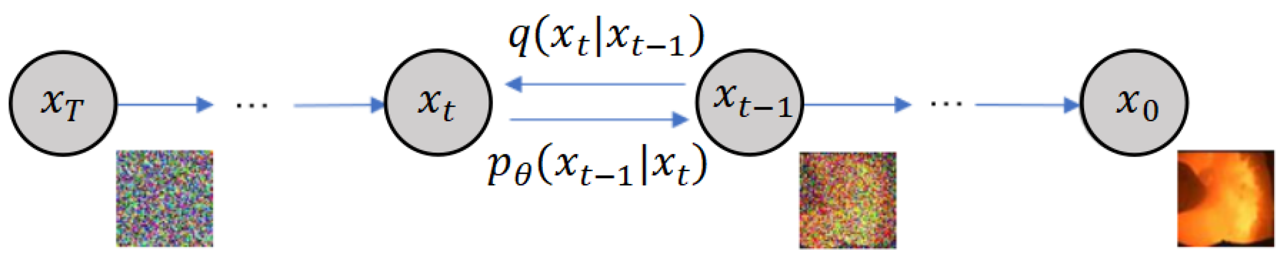
Deep learning requires a large amount of balanced data with different sample numbers to support model training. However, abnormal burning conditions are rare in the field, and it is very difficult to collect a large amount of data with uniform distribution. Therefore, scholars have proposed the use of image generation models to expand training data to address this issue. Qiu et al. [11] established a VAE model to reconstruct a large amount of generated data by using flame images collected from coal-fired boilers as input and processed through an encoder and decoder. Recently, the image generation method based on Denoising Diffusion Probabilistic Models (DDPMs) has made great progress [12], and its potential in expanding image datasets has been increasingly recognized by scholars. Many scholars have begun to use this method to address the problem of uneven distribution of image sample data. Lee and Yun [13] proposed a DDPM to generate images similar to datasets including several different types of microstructures (such as polycrystalline alloys, carbonates, ceramics, copolymers, fiber composites, etc.). Khader et al. [14] proposed the generation magnetic resonance images (MRIs) and computed tomography (CT) images using a DDPM and demonstrated that the generated images can be used to train image segmentation models. Yilmaz et al. [15] proposed a method for generating microscope image data that can effectively generate fully annotated microscope image datasets by establishing a DDPM and training the model. This helps reduce the reliance on manual annotation when training deep learning-based segmentation methods, enabling the segmentation of different datasets without the need for manual annotation. Khanna et al. [16] improved an original network based on a DDPM to address the spatiotemporal characteristics of remote sensing data and proposed the DiffusionSat model for the generation satellite remote sensing images. Asya et al. [17] proposed the GradPaint method to generate a coordinated image by calculating a custom loss to measure its consistency with the masked input image. Existing diffusion-based inpainting methods are limited to single-modal guidance and require task-specific training, hindering their cross-modal scalability. To solve this problem, Yang et al. [18] proposed the Uni-paint generation model. Uni-paint is based on pre-trained stable diffusion and does not require task-specific training on a specific dataset, achieving a few-shot generalization capability on custom images.

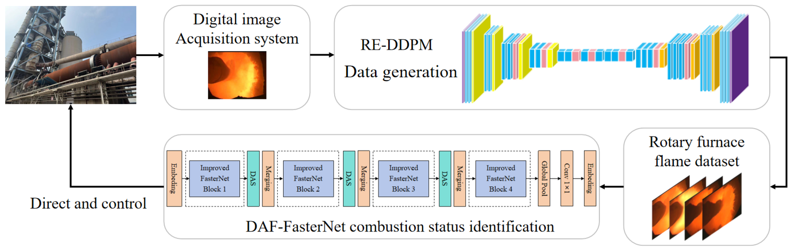
This article proposes a flame combustion image generation method based on RE-DDPM to address the problems of insufficient data and severely uneven sample distribution. In this paper, the RE-DDPM method is used to generate a large number of images that are extremely similar to real data based on a small number of live burning strip images, solving the problem of insufficient training samples for deep learning. Experiments show that following the use of the method proposed in this paper to expand the data, the generated data are more similar to the real data, and the recognition accuracy of the model can be improved. Secondly, to address the problem of low accuracy in combustion state recognition, a combustion state recognition method based on DAF-FasterNet is proposed. This article improves upon the original FasterNet network [19] to significantly improve recognition accuracy while ensuring recognition speed. Extensive experiments show that the combustion state recognition method proposed in this paper has advantages in terms of both speed and accuracy.

The main contributions of this research can be summarized as follows:

• A new model for recognizing the combustion state of cement rotary kilns is proposed. This model first addresses the problem of a small dataset and uneven sample distribution through RE-DDPM. Then, it achieves precise and fast recognition of the combustion state through DAF-FasterNet.
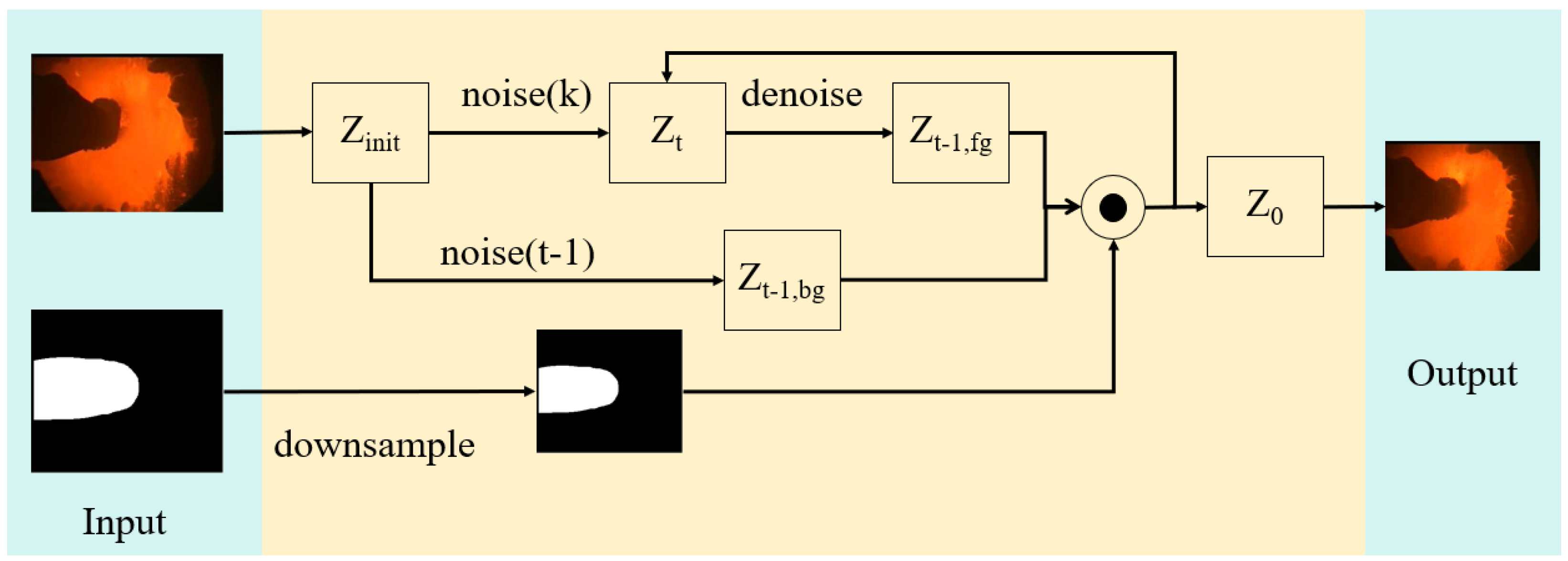
• This paper proposes a new image generation method, RE-DDPM. During training, a mask operation is applied to a part of the original image, and the mask is also included as input, achieving local redrawing of the image. This makes the generated data more consistent with real scenes. The proposed local redrawing method outperforms traditional redrawing methods.
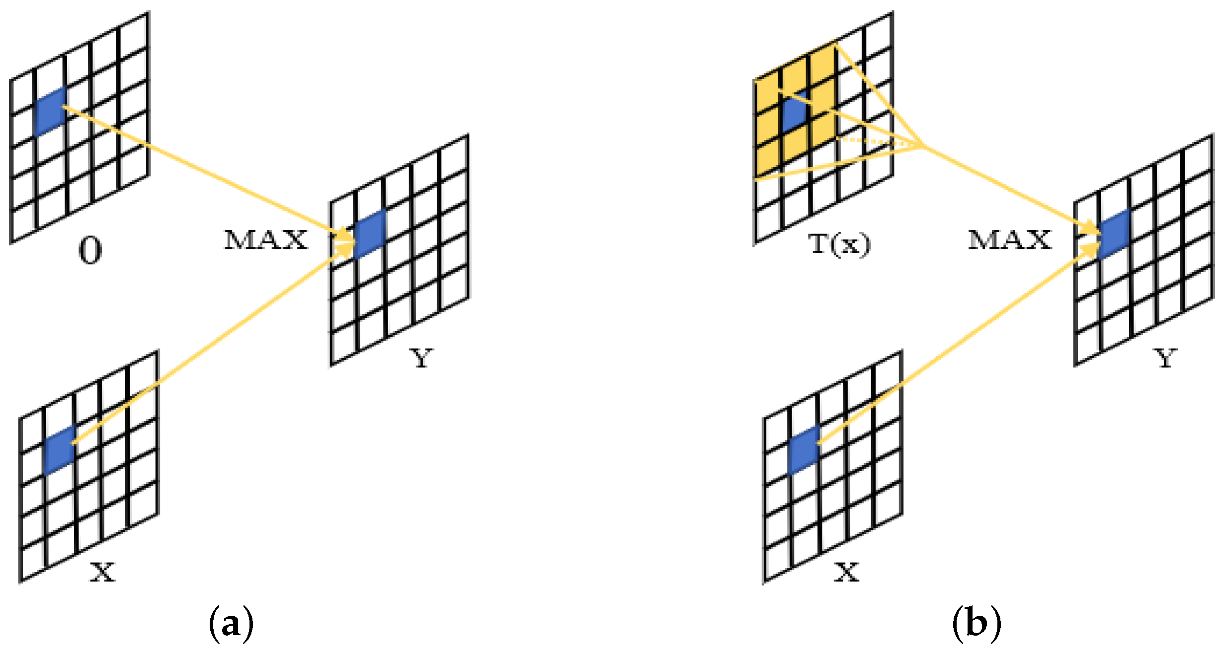
• This paper proposes a new method for recognizing the combustion state of flames, DAF-FasterNet. By improving the activation function in FasterNet to FReLU, the activation function gains the ability to capture spatial layouts, improving the model’s recognition accuracy. Additionally, a lightweight attention DAS is introduced, making the model pay more attention to the combustion characteristics of flames. This not only ensures the lightweight nature of the model but also further improves recognition accuracy.

3. Preliminaries

This section describes the original deep learning models, DDPM and FasterNet. First, we introduce the image generation principle of DDPMs and the deep learning training network, U-net, used in them. Then, we introduce the network structure of FasterNet and the novel convolution method, PConv, used in FasterNet.

3.1. Denoising Diffusion Probabilistic Models

Denoising diffusion probabilistic models (DDPMs) have emerged as prominent generative models in recent years, recognized for their superior quality and diversity in image generation. The training process of DDPMs is more stable than that of GANs, and there are no problems such as mode collapse or mode drop. The algorithm consists of two processes: the forward process and the reverse process [20,21] (Figure 1).

Figure 1. Schematic diagram of DDPM training.

The forward process (from $x_0$ to $x_T$ in Figure 1) is the process of adding noise to the image. Given a real image sample ($x_0\sim q\left(x\right)$), the forward process adds Gaussian noise to it for T steps, resulting in $x_1,x_2,x_3\dots \dots x_T$. The size of each step is controlled by a series of hyperparameters (${\left\{{\beta }_t\in \left(0,1\right)\right\}}_{t=1}^T$) of the Gaussian distribution variance. Since each moment (t) in the forward process only depends on the moment ($t-1$), it can also be seen as a Markov chain process:

$$q\left(x_t\mid x_{t-1}\right):=N\left(x_t;\sqrt{1-{\beta }_t}{x}_{t-1},{\beta }_{t}I\right),$$

(1)

where the value of $\beta$ varies with time. For example, ${\beta }_1$ is small, ${\beta }_t$ is large, and I is the identity matrix.

The reverse process is the denoising inference process. If it is possible to reverse the forward process and sample from $q\left(x_{t-1}\mid x_t\right)$, it is possible to gradually approach the original image distribution ($x_0\sim q\left(x\right)$) from the Gaussian noise ($x_T\sim N\left(0,1\right)$). Abbeel et al. [12] showed that if $q\left(x_t\mid x_{t-1}\right)$ follows a Gaussian distribution and ${\beta }_t$ is small enough, $q\left(x_{t-1}\mid x_t\right)$ follows a Gaussian distribution. However, we cannot simply infer $q\left(x_{t-1}\mid x_t\right)$, so scholars use a deep learning model (U-Net) to predict such a reverse distribution ($p_{\theta }$):

$$p_{\theta }\left(x_{t-1}\mid x_t\right):=N\left(x_{t-1}\mid {\mu }_{\theta }\left(x_t,t\right),{\sum }_{\theta }\left(x_t,t\right)\right),$$

(2)

where the mean ${\mu }_{\theta }$ and variance ${\sum }_{\theta }$ are both calculated according to the model. By considering all time steps and according to the Markov chain, the reverse process can be derived, as shown in Equation (3):

$$p_{\theta }\left(x_{0,T}\right)=p\left(x_T\right)\prod _{i=1}^T{p}_{\theta }\left(x_{t-1}\right|x_t),$$

(3)

DDPMs use a U-Net neural network [22] for training (Figure 2). The network consists of downsampling layers, middle layers, and upsampling layers. In the downsampling layers, two residual blocks are inserted before each downsampling operation. The number of channels is doubled in each downsampling layer, except for the last step. The structure of the upsampling layers is symmetrical to that of the downsampling layers, but three residual modules are added before each upsampling operation. Unlike the downsampling layers, three residual blocks are used before each upsampling operation.

Figure 2. U-Net network architecture.

3.2. FasterNet

There are some redundant calculations in the structure of deep convolutional neural networks, which lead to a larger amount of floating-point operations FLOPs, thereby increasing the model’s latency. The relationship between latency, FLOPs, and FLOPS’ is expressed as follows [19]:

$$Latency={\displaystyle \frac{\mathrm{FLOPs}}{\mathrm{FLOPS}}},$$

(4)

where FLOPs are floating-point operations and FLOPS stands for floating-point operations per second. The calculation latency is determined by FLOPs and FLOPS.

It is easy to see from Equation (4) that the goal of improving detection speed can be achieved by reducing FLOPs and increasing FLOPS. FasterNet differs from traditional lightweight neural networks MobileNet [23], ShuffleNet [24], and GhostNet [25] by providing a convolutional method, Partial Convolutional (PConv), that significantly reduces model identification latency.

3.2.1. FasterNet Network Architecture

Each FasterNet module consists of one PConv layer and two Pointwise Convolution [23] (PWConv) layers. In addition, normalization and activation layers play a crucial role in neural networks and are indispensable components. The two PWConv layers in each FasterNet module are equipped with Batch Normalization (BN) and rectified linear units (ReLUs). Many researchers [26,27] overuse batch normalization (BN) layers and ReLU layers in neural networks, which leads to reduced feature diversity and further affects model performance. It also slows down the overall computation. The original authors used these layers only after each intermediate PWConv to maintain feature diversity and achieve lower latency.

3.2.2. PConv

In FasterNet, PConv only needs to apply conventional convolution to a part of the input channel to extract spatial features. The remaining channels remain unchanged. If the feature map is stored continuously or regularly in memory, the first or last continuous channel is considered to be representative of the entire feature map. When comparing the performance of Conv with PConv on GPU, CPU, and ARM devices, PConv shows lower Latency. A comparison between conventional convolution and PConv is shown in Figure 3.

Figure 3. (a) A standard convolution operation; (b) A partial convolution operation.

The computational complexity and memory access of Conv are shown in Equations (5) and (6), and the computational complexity and memory access of PConv are shown in Equations (7) and (8):

$$h\times w\times k^2\times c^2,$$

(5)

$$h\times w\times 2c+k^2\times c^2\approx h\times w\times 2c,$$

(6)

$$h\times w\times k^2\times c_p^2,$$

(7)

$$h\times w\times 2c_p+k^2\times c_p^2\approx h\times w\times 2c_p,$$

(8)

where $c_p$ is the channel where the convolution operation has is performed ($c>c_p$).

According to the experimental results, compared to conventional convolution, PConv achieves a significant reduction in FLOPs, requiring only 1/16 of the computational operations. Similarly, memory access in PConv is reduced to 1/4 of that in conventional convolution.

The FasterNet network structure is shown in Figure 4.

Figure 4. FasterNet structure.

4. Methodology

The proposed combustion state recognition model combines the improved RE-DDPM and DAF-FasterNet, as shown in Figure 5. Images of the rotary kiln collected on site are used as inputs for RE-DDPM. A feature extractor in RE-DDPM extracts image features and generates new rotary kiln images using the learned features. The newly generated images are used as the training set for the recognition network, DAF-FasterNet, while all the actual images collected on site are used as the validation set for DAF-FasterNet, ensuring the effectiveness of the training results.

Figure 5. Combustion state detection method for cement rotary kilns.

4.1. RE-DDPM

During on-site data processing, it was found that the information of the feed-inlet and furnace-wall parts does not play a key role in combustion state recognition. In the training of the recognition network, the identical feed inlet and furnace wall reduce the network’s focus, thereby making the network pay more attention to the important flame combustion area and improving recognition accuracy. Moreover, generating diversity in non-critical parts such as the feed inlet and furnace wall may lead to significant deviations between the generated data and actual on-site data, resulting in decreased combustion state recognition accuracy. Therefore, the data generation method needs to be optimized, allowing the DDPM to achieve partial redrawing so that the generated data better match the actual situation. The existing local redrawing method [28] adds a mask to the areas of the initial image that need to be redrawn, allowing the DDPM to generate only within the masked area while keeping the rest of the image unchanged. This local redrawing method focuses solely on the feature distribution within the redrawn area, without considering the feature distribution relationship between the redrawn area and other regions. This results in a very noticeable disconnection at the boundaries between the redrawn area and other regions, causing the redrawn image to significantly deviate from the real data. Therefore, this paper redesigns the local redrawing method and modifies the network’s input to achieve local redrawing that better aligns with real data. First, the image mask is also used as input. Then, the noise level of the initial image is increased to the required noise level, and the denoising diffusion process is manipulated as follows (the algorithm is shown in Figure 6):

Figure 6. RE-DDPM.

• In each step, the denoising step is first perofrmed to obtain a less noisy foreground, which is denoted as $Z_{t-1,fg}$.
• Simultaneously, add noise ($Z_{init}$) is added to the current noise level to obtain a noisy background ($Z_{t-1,bg}$).
• Then, the adjusted mask (m) is used to blend $Z_{t-1,fg}$ and $Z_{t-1,bg}$, denoted as $Z_{t-1,fg}\odot m+Z_{t-1,bg}\odot \left(1-m\right)$, to produce the image for the next denoising step.

The method proposed in this article blends masked and unmasked regions with the same noise level during the training process. Therefore, the network focuses on the distribution of data in the entire image. In contrast, existing local redrawing methods only train the masked redrawn parts, thereby neglecting the relationship between the redrawn and non-redrawn parts in the data distribution. Compared with existing methods (such as variational autoencoders and generative adversarial networks), the images generated by the proposed method are more realistic and more in line with human perception.

Additionally, this paper improves the network’s attention mechanism by adding self-attention mechanisms to the 32 × 32, 16 × 16, and 8 × 8 layers, not just the 16 × 16 layer. This allows the network to focus on deeper features of the image, such as flame textures and color gradients. As a result, the quality of data generation is improved.

4.2. DAF-FasterNet

Through the analysis of the flame-burning image data, it was found that the local flame distribution is one of the important characteristics of the burning state [29]. However, FasterNet fails to capture this feature, leading to lower recognition accuracy. Therefore, this paper proposes an improvement based on FasterNet called DAF-FasterNet for combustion state recognition. In this section, we introduce our improvement method.

4.2.1. Funnel Activation-FReLU

Research on actual image data has found that the distribution of flames exhibits regional characteristics and that the variation between regions is also one of the features of flame combustion states [29]. In response to this characteristic, this paper proposes improvements to the original network. The original FasterNet block, after convolution, uses ReLU [30] as the activation function. Although ReLU is the most widely used activation function, experiments have shown that its insensitivity to spatial information hinders further improvement in accuracy. Therefore, this paper improves ReLU by replacing it with an activation function specifically designed for visual tasks called FReLU [31] to address this limitation. The original ReLU uses $max\left(·\right)$ to perform the nonlinear operation, where the condition is manually set to 0, so the form of ReLU is $y=max\left(x,0\right)$. Zhang et al. improved recognition accuracy by adding a 2D funnel-shaped spatial condition ($T\left(x\right)$) that depends on spatial context to the activation function, allowing it to extract the precise spatial layout of objects. To implement the spatial condition, the authors used parameter pooling windows to create spatial dependencies.The comparison between ReLU and FReLU is shown in Figure 7. Therefore, the new activation function takes the form shown in Equations (9) and (10).

$$y\left(x_{c,i,j}\right)=max(x_{c,i,j},T\left(x_{c,i,j}\right)),$$

(9)

$$T\left(x_{c,j,j}\right)=x_{c,j,j}^w·p_c^w,$$

(10)

Figure 7. (a) represents ReLu: $y=max\left(x,0\right)$; (b) represents FReLu: $y=max\left(x,T\left(x\right)\right)$.

In Equations (9) and (10), $x_{c,i,j}$ represents the input pixel of the nonlinear activation function ($y\left(·\right)$) in channel c of the 2D spatial position ($\left(i,j\right)$). The function $T\left(·\right)$ represents the funnel condition. $x_{c,j,j}^w$ represents the parameter pooling window ($k_h\times k_w$) centered at $x_{c,i,j}$. $p_c^w$ denotes the window coefficient shared within the same channel.

Therefore, FReLU generates spatial dependencies while performing nonlinear activation, with activation dependent on spatial conditions. Utilizing the properties of the spatial condition ($T\left(x\right)$) and the function expressed as $max\left(·\right)$, FReLU can provide spatial layout capabilities, naturally and easily extracting the spatial structure of objects, thereby enhancing the network’s recognition accuracy.

4.2.2. Deformable Attention to Capture Salient Information—DAS

In the original FasterNet, the authors did not design an attention mechanism, resulting in low accuracy in handling combustion state recognition tasks. The attention mechanisms in convolutional neural networks can be roughly divided into channel attention, spatial attention, and mixed-domain attention. These methods use techniques such as aggregation, subsampling, and pooling to include specific attention computations, which, while improving recognition accuracy, significantly increase the computational load of the model. For industrial production scenarios, due to limitations in computing equipment or the requirement for low latency, these attention mechanisms are challenging to satisfy. Therefore, a lightweight attention mechanism, DAS [32] (structure shown in Figure 8), was introduced to improve FasterNet, enhancing recognition accuracy while maintaining a lightweight design.

Figure 8. DAS attention mechanism.

First, a depthwise separable convolution (DSC) is used as a bottleneck layer. This convolution method reduces the number of channels in the feature map, converting their number from c to $\alpha \times c$. c is the selected dimension reduction parameter, balancing computational efficiency and accuracy (generally, $0<\alpha <1$). Extensive experimental results have shown that $\alpha =0.2$ is the optimal choice [31].

After the bottleneck layer, instance normalization layer is applied. This process removes instance-specific contrast information from the image, improving the robustness of deformable convolution attention during training. This is followed by GELU nonlinear activation. These operations enhance the representation capability of the features, contributing to the effectiveness of the attention mechanism. Equation (11) represents the normalization compression process, where X is the input feature and $W_1$ is the depthwise separable convolution.

$$X_c=GELU\left(Instancenorm\left(X{W}_1\right)\right),$$

(11)

The compressed feature data, after being compressed by Equation (11), represent the feature context and are then passed through a deformable convolution (DC). This convolution uses a dynamic grid (offset $△p$) instead of a regular grid, which helps focus on relevant image regions. Equation (12) presents the operation of the deformable convolution kernel, where k is the kernel size and its weights are applied at fixed reference points in $p_{ref}$, similar to the regular kernel in a CNN. $\mathsf{\Delta }p$ is a trainable parameter that helps the kernel find the most relevant features, even if they are outside the reference kernel. $w_p$ is another trainable parameter between 0 and 1. The values of $\mathsf{\Delta }p$ and $w_p$ depend on the features on which the kernel function operates.

$$deform\left(p\right)=\sum _{k=1}^k{w}_k·w_p·X(p_{ref,k}+\mathsf{\Delta }{p}_k),$$

(12)

After the deformable convolution, layer normalization is applied. Then, a Sigmoid activation function ($\sigma$) is used (as shown in Equation (13)). This convolution operation changes the number of channels from $\alpha \times c$ to the original input (c).

$$A=\sigma \left(LayerNorm\left(deform\left(X_c\right)\right)\right),$$

(13)

The output of Equation (13) represents an attention gate. This gate controls the flow of information from the feature map, with each element’s value in the gate tensor ranging from 0 to 1. These values determine which parts of the feature map are emphasized or filtered out. Finally, to integrate the DAS attention mechanism into the CNN model, the method performs element-wise multiplication between the original input tensor and the attention tensor obtained in the previous step.

$$X_{out}=X\odot A,$$

(14)

The result of the multiplication in Equation (14) is the input of the next layer of the CNN model, seamlessly integrating the attention mechanism without needing to change the backbone architecture.

Furthermore, this article expands the receptive field of PConv by improving the single-layer 3 × 3 PConv to a double-layer 9 × 9 PConv, allowing it to better capture spatial distribution features. The DAF-FasterNet network structure proposed in this paper is shown in Figure 9.

Figure 9. DAF-FasterNet network architecture.

5. Experiments

To validate the effectiveness and superiority of the cement rotary kiln flame combustion state recognition method proposed in this paper, a large number of experiments were conducted. The experiments reported in this paper were conducted under the following conditions: operating system: Windows 10; CUDA: 11.0; GPU: RTX 3080; CPU: i7-12700KF; framework: PyTorch 2.0.1.

The image generation model was trained on each dataset for 500 epochs, and the batch size was set to 16. For the first 200 epochs, a learning rate of $1.0\times {10}^{-4}$ was used, followed by a learning rate of $2.0\times {10}^{-5}$ for the next 300 epochs. We choose the Adam optimizer (${\beta }_1$ = 0.9, ${\beta }_2$ = 0.999) to train the L1 loss function. We trained the FasterNet recognition model for 300 epochs, the batch size was set to 32, the learning rate was set to $1.0\times {10}^{-4}$, and the AdamW optimizer was used.

5.1. Evaluation Metrics

The evaluation metrics proposed in this paper consist of two parts: image generation evaluation metrics and neural network evaluation metrics. They are used to demonstrate the superiority of the RE-DDPM and DAF-FasterNet proposed in this paper.

5.1.1. Flame Image Generation Evaluation Metrics

We use Structural Similarity (SSIM) as one of the evaluation criteria for image generation quality [33].

$$\mathrm{SSIM}(X,Y)={\displaystyle \frac{(2{\mu }_X{\mu }_Y+c_1)(2{\sigma }_{XY}+c_2)}{({\mu }_X^2+{\mu }_Y^2+c_1)({\sigma }_X^2+{\sigma }_Y^2+c_2)}},$$

(15)

where $m{u}_X$ and $m{u}_Y$ represent the mean pixel intensities of images X and Y, respectively; ${\sigma }_X^2$ and ${\sigma }_Y^2$ represent the pixel-intensity variances of X and Y, respectively; ${\sigma }_{XY}$ represents the covariance of images X and Y; and $c_1$ and $c_2$ are two variables for stable division.

The Frechet Inception Distance (FID) score is a metric that calculates the distance between the feature vectors of real and generated images [34]. A lower score indicates that the two sets of images are more similar or that their statistics are more similar. The FID score is 0.0 in the best case scenario, indicating identical images.

$$\mathrm{FID}(X,Y)=\left|\right|m{u}_X-m{u}_Y{\left|\right|}^2+Tr(C_X+C_Y-2\ast sqrt(C_X\ast C_Y)),$$

(16)

where $m{u}_X$ and $m{u}_Y$ represent the feature means of the real and generated images and $C_X$ and $C_Y$ represent the covariance matrices of the actual feature vectors and the generated feature vectors.

The Learned Perceptual Image Patch Similarity LPIPS can also evaluate the distortion of generated images. LPIPS essentially calculates the similarity between activations of two image patches in a predefined network. LPIPS can be defined as follows:

$$\mathrm{LPIPS}(X,Y)={\sum }_l{\displaystyle \frac{1}{H_l{W}_l}}{\sum }_{h,w}\left|\right|w_l\odot ({\widehat{X}}_{hw}^l-{\widehat{Y}}_{hw}^l){\left|\right|}_2^2,$$

(17)

where $H_l$ and $W_l$ are the height and width of the input features in layer l of the predefined network, respectively. $W_l$ is the weight of each feature in layer l. ${\widehat{X}}_{hw}^l$ and ${\widehat{Y}}_{hw}^l$ represent the normalized features of pixel $\left(h,w\right)$ in layer l. ⊙ multiplies the feature vector at each pixel by the feature weight.

5.1.2. Flame Combustion State Recognition Evaluation Metrics

For the requirements of the cement rotary kiln production scene, high accuracy (ACC) is one of the most important requirements. The formula for calculating accuracy is shown in Equation (18):

$$ACC={\displaystyle \frac{(TP+TN)}{(P+N)}},$$

(18)

where $TP$ represents true positives; $TN$ represents true negatives; and P and N are the total numbers of positives and negatives, respectively.

Due to the limitations of computing equipment in production scenarios, the computational load of the model (FLOPs) also needs to be considered. Large models are difficult to deploy in practice, so it is necessary to reduce model complexity while ensuring recognition accuracy. Additionally, high latency is unacceptable in real production, as it can lead to significant economic losses and potential production safety hazards.

In summary, accuracy and parameter count and latency are used as the basis for evaluating neural network recognition methods.

5.2. Data Preparation

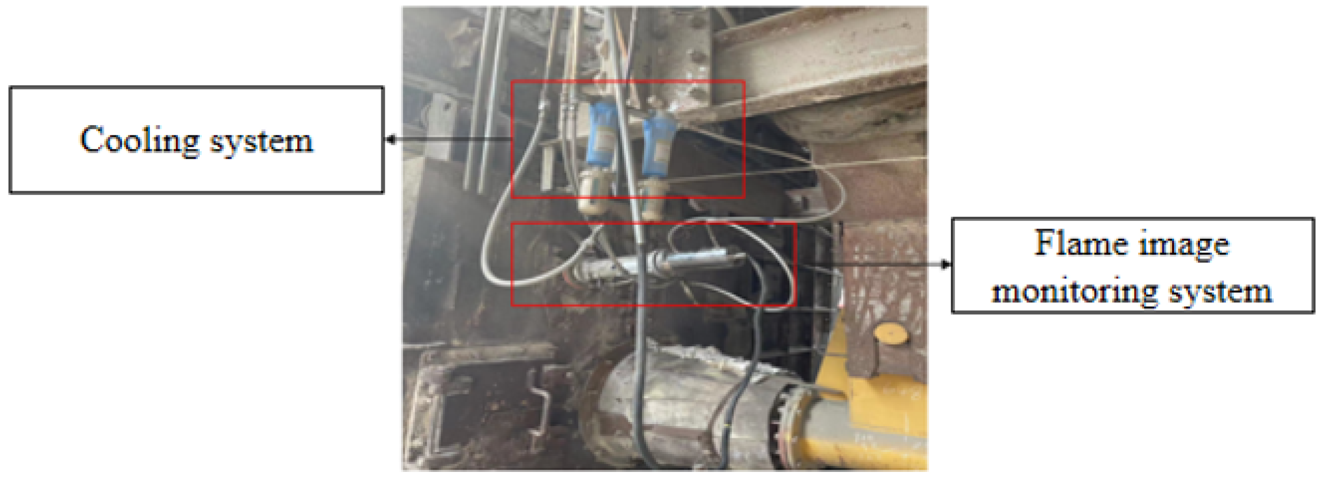
The flame image monitoring device (CCD camera and cooling system) was installed in the cement rotary kiln of a cement plant, as shown in Figure 10. A color CCD camera (resolution: 1920 × 1080; refresh rate: 30 FPS) was used to collect the burning data, and the subsequent detection of the burning state was carried out. A cooling system was used to reduce the temperature of the camera’s operating environment to ensure the normal operation of the equipment. The resolution of the collected image is 1920 × 1080, which is sufficient to reflect the detailed distribution characteristics, texture characteristics, and color characteristics of the flame.

Figure 10. Cement rotary kiln combustion detection system.

The data collected on site were manually annotated by experts, classifying the combustion state in the combustion zone into three categories: normal sintering, under-sintering, and over-sintering. The on-site images of each condition are shown in Figure 11. The distribution of data samples collected by the monitoring device is shown in Table 1.

Figure 11. (a) Under-sintering; (b) normal sintering; (c) over-sintering.

Table 1. Distribution of combustion state data.

Category	Normal Sintering	Over-Sintering	Under-Sintering	Total
Quantity	1538	165	142	1845

The data in the table indicate a severe imbalance in sample distribution, and the data volume is completely insufficient to support deep learning training. Therefore, it is necessary to expand the data samples to achieve a balanced sample distribution to meet the needs of deep learning training.

Due to the high-temperature environment inside the furnace, some images have significant noise and require denoising processing. In this study, a Gaussian filter was used for denoising. Through analysis of the sample data, it was found that the contribution of the furnace wall edges to the classification is very small. Therefore, the images were cropped around the discharge port to 1080 × 1080. This not only reduces network training time but also reduces the interference of some unimportant factors.

5.3. Experimental Results

To verify the feasibility of the method, optimize the data generation part, and improve the detection method, we conducted experiments on the flame combustion state model of a cement rotary kiln based on RE-DDPM and DAF-FasterNet. The initial DDPM and FasterNet model were evaluated, and the performance after improvement for these two parts was studied. Additionally, we conducted a large number of comparative and ablation experiments, comparing the results obtained with the proposed methods. The research results include SSIM, FID, and LPIPS for the image generation part and ACC, FLOPs, and latency for the detection part.

5.3.1. Flame Image Generation

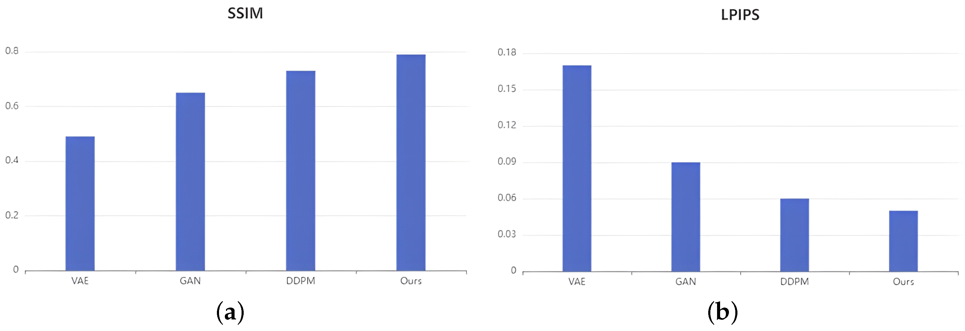
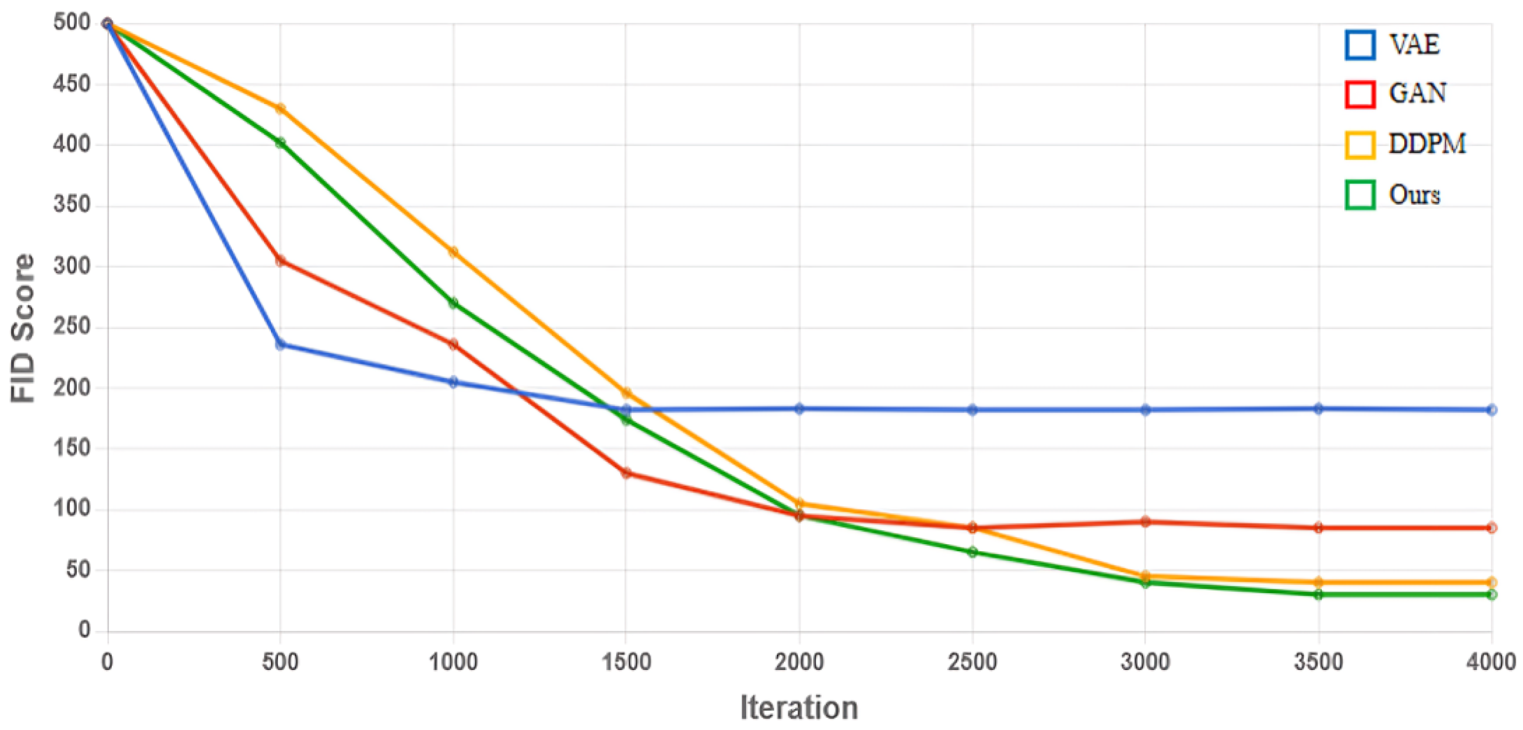
We compared our proposed method with other neural networks (GAN, VAE, and original DDPM). Figure 12 shows the performance of each model. In terms of SSIM, DDPM outperforms GAN and VAE, and our method, RE-DDPM, outperforms the original DDPM. In terms of LPIPS, our method achieved the lowest score, indicating that the images generated by our method are more in line with human perception. Figure 13 shows the FID scores for certain iterations, with the FID scores gradually decreasing with an increasing number of iterations. A lower FID score indicates more similarity, as the FID score between two identical datasets is almost zero.

Figure 12. (a) Score for each model in terms of structural similarity; (b) score for each model in terms of learned perceptual image-patch similarity.

Figure 13. FID change graph.

Although the DDPM shows promise in data augmentation, the sampling speed is still much slower compared to GAN and VAE. A GAN consists of a discriminator and a generator. The generator is responsible for generating images, while the discriminator is used to judge the authenticity of the generated images. A trained GAN model can directly generate target images in one step. However, unlike aa GAN, a DDPM recovers images from noise in the form of a Markov chain in the reverse denoising process. This means that the more iterations we set, the longer it takes to generate images. Nevertheless, the images generated by a DDPM still achieve satisfactory results. Furthermore, due to improvements in network attention and the use of local redrawing methods in our method, the images generated by the model are more realistic, and the training speed of the network is also improved.

Figure 14 shows images generated by different models. The images generated by VAE are too blurry to display the rich details of flame images. Compared to the DDPM, VAE’s loss function typically includes a reconstruction loss, which measures the difference between the images generated by the decoder and the original input images. This reconstruction loss helps the model learn the data distribution but may result in generated images lacking detail and clarity, especially for complex structures or high-resolution images. Additionally, VAE assumes that the latent space is continuous, meaning that similar latent vectors generate similar images. This continuity may cause the model to converge to some blurry intermediate representations when generating images rather than producing clear images. The images generated by a GAN differ significantly from the real images in the distribution of flame texture features. The original DDPM achieves satisfactory results in terms of clarity and diversity, but there are significant differences in flame texture details compared to real images. For example, in the images of normal sintering generated by the original DDPM, there are large areas of bright flames, which severely deviate from the actual distribution of flames in real images and may cause the recognition network to identify them as over-sintering, reducing recognition accuracy. The images generated by our RE-DDPM are closer to real images.

Figure 14. (a) Reference image; (b) image generated by VAE; (c) image generated by GAN; (d) image generated by DDPM; (e) image generated by RE-DDPM. Significant regions are highlighted with red boxes.

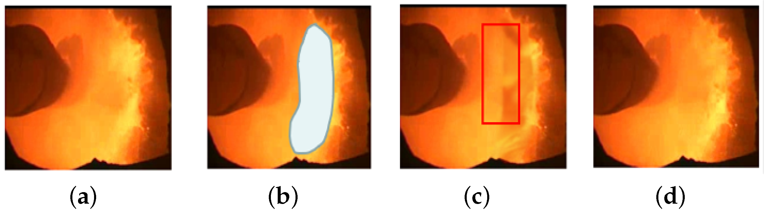
Traditional local redrawing focuses on the global generation of the redrawn region and does not consider the data distribution relationship between the redrawn region and other regions. This can cause a noticeable discontinuity at the boundary between the two regions, as shown in Figure 15. When RE-DDPM performs local redraw, it considers the distribution of flame characteristics between the redrawn region and other regions. Our proposed redrawing method can maintain the consistency around the furnace wall while achieving high similarity and diversity in the redrawn flame region. The generated images appear more realistic and natural at the boundary between the redrawn region and other regions.

Figure 15. (a) Input image; (b) the addition of a mask to the image; (c) image generated by traditional local redrawing; (d) image generated by our proposed local redrawing method. Significant regions are highlighted with red boxes.

We also conducted ablation experiments on the improvement of the attention module in the U-Net network, with evaluation metrics including SSIM, LPIPS, and FID, to demonstrate that our improvements, indeed, enhance the generation effect. While adding more self-attention distributions may increase the computational cost of model training and slow down the training speed, it allows the network to extract more effective features, resulting in generated images with richer textures that better match the on-site images. The original U-Net’s attention mechanism is distributed in 16 × 16 layers. We improved it to 32 × 32, 16 × 16, and 8 × 8 layers. The specific performance is shown in Table 2.

Table 2. U-Net network attention distribution experiment.

Category	Resolution Layers	SSIM	LPIPS	FID
1	[]	0.60825	0.062	44
2	[16]	0.66372	0.056	39
3	[8,16]	0.73625	0.059	36
4	[16,32]	0.67491	0.051	42
5	[8,16,32]	0.76335	0.049	34

Using the image generation method we proposed, we expanded the original collected dataset. The normal combustion data were reduced to 1000 images, while the over-sintered images were increased to 1000 images and the under-sintered images were also increased to 1000 images. We partitioned the dataset such that 80% was used as the training set, 10% as the test set, and 10% as the validation set.The sample distribution of the expanded dataset is shown in Table 3.

Table 3. Distribution of the augmented combustion state data.

Category	Normal Sintering	Over-Sintering	Under-Sintering	Total
Quantity	1000	1000	1000	3000

In order to verify the effectiveness of the proposed image generation method in augmenting the dataset, experiments were conducted on the original data, DDPM-augmented data, and RE-DDPM-augmented data. The experimental results demonstrate the effectiveness of the proposed method.The experimental results are shown in Table 4.

Table 4. Recognition accuracy for different datasets.

Dataset	Recognition Method	Accuracy
Original dataset	FasterNet	87.2%
DDPM dataset	FasterNet	91.4%
RE-DDPM dataset	FasterNet	93.1%

5.3.2. Combustion State Recognition

To validate the accuracy and speed optimization of the method in the detection of combustion states in cement rotary kilns, we first conducted comparative experiments on different backbones to verify the superiority of the proposed method. The specific experimental results are shown in Table 5. Although FasterNet does not have a significant advantage in Params and FLOPs, it achieves excellent scores in latency, being 35.4 ms faster than the most widely used ResNet. Furthermore, compared to other lightweight networks such as MobileNet and ShuffleNet, FasterNet still achieves better results. MobileNet, ShuffleNet, GhostNet, and other networks use depthwise convolution (DWConv) and/or group convolution (GConv) to extract spatial features. However, in the process of reducing FLOPs, operators often suffer from the side effects of increased memory access. Additionally, these networks are often accompanied by additional data operations such as concatenation, shuffling, and pooling, which are often important for small models in terms of runtime. Our method improves the structure and receptive field of the network based on FasterNet. We upgraded the single-layer PConv to a double-layer and improved the receptive field from 3 × 3 to 9 × 9. Experimental results show that while there is no significant increase in parameters or computational complexity, the recognition accuracy is improved.

Table 5. Experimental comparison of different backbones.

Network	Params (M)	FLOPs (G)	Latency (ms)	ACC (%)
GhostNet	7.3	0.23	20.1	92.3
ShuffleNetV2	7.4	0.58	17.6	90.5
MobileNetV2	6.1	0.58	21.4	91.3
MobileVit-XS	2.3	1.03	40.5	90.8
ResNet-18	11.5	1.82	52.6	93.2
FasterNet	7.6	0.85	16.9	93.1
Ours	7.6	0.86	17.2	93.7

After improvement, FasterNet can achieve an accuracy of 93.7% in recognition accuracy, but it still cannot meet the requirements of actual production. One reason is the lack of an attention mechanism in the original network. To address the issue of low recognition accuracy, we propose the introduction of a lightweight attention mechanism, DAS, to improve the network. This improvement not only ensures that the model is lightweight but also improves the recognition accuracy. The experimental results are shown in Table 6. The proposed improvement method increases the parameters by only 0.13 M and the FLOPs by only 0.01 G compared to the original network while improving the accuracy by 2.7%. We also compared it with other common attention mechanisms, such as SENet, BAM, and CBAM, demonstrating the significant superiority of the proposed improvement method.

Table 6. Experimental comparison of different attention mechanisms.

Network	Params (M)	FLOPs (G)	Latency (ms)	ACC (%)
None	7.6	0.86	17.2	93.7
+SENet	7.78	0.86	21.5	95.3
+BAM	7.73	0.87	20.4	94.9
+CBAM	7.91	0.90	22.1	94.4
+Triplet Attention	7.78	0.88	20.5	95.1
+DAS	7.73	0.87	21.3	96.4

To validate the effectiveness of our improvement of the activation function in FasterNet, we replaced all ReLU activation functions in the network with FReLU visual activation functions and conducted experiments. The experimental results are shown in Table 7. Additionally, we compared it with other activation functions, such as ReLU, PReLU, and Swish, demonstrating that the improvement proposed in this paper has a significant advantage in accuracy.

Table 7. Comparison of results obtained with different activation functions.

Model	Activation	Params (M)	FLOPs (G)	Latency (ms)	ACC (%)
Ours + DAS	+ReLU	7.73	0.87	21.3	96.4
	+PReLU	7.91	0.87	22.5	97.1
	+Swish	7.86	0.88	23.4	96.9
	+Leaky ReLU	8.05	0.91	24.1	97.2
	+FReLU	7.86	0.88	23.7	98.4

6. Conclusions

The improved DDPM and FasterNet networks successfully passed testing. Experimental results indicate that our method demonstrates significant advantages in terms of clarity and realism in generating cement rotary kiln flame images compared to other models. The high-quality generated data lay a solid foundation for the accurate recognition of subsequent identification networks. Similarly, in terms of combustion state recognition, our model utilizes the FasterNet network as the backbone structure to reduce network redundancy and memory access, thereby improving the model’s speed. Additionally, we introduced the DAS attention mechanism and improved activation functions, which significantly enhanced the accuracy of combustion state recognition without a noticeable increase in latency. In conclusion, the method proposed in this paper provides a new model for faster and more accurate recognition of rotary kiln flame combustion states.