Early Detection of Surface Mildew in Maize Kernels Using Machine Vision Coupled with Improved YOLOv5 Deep Learning Model

Abstract

Mildew in maize kernels is typically caused by various fungi, necessitating prompt detection and treatment to minimize losses during harvest and storage. In this study, a deep learning YOLOv5s algorithm based on machine vision technology was employed to develop a maize seed surface mildew detection model and to enhance its portability for deployment on additional mobile devices. To guarantee the fruitful progression of this research, an initial experiment was conducted on maize seeds to obtain a sufficient number of images of mildewed maize kernels, which were classified into three grades (sound, mild, and severe). Subsequently, a maize seed image was extracted to create an image of a single maize seed, which was then divided to establish the data set. An enhanced YOLOv5s–ShuffleNet–CBAM model was ultimately developed. The results demonstrated that the model achieved with an mAP50 value of 0.955 and a model size of 2.4 MB. This resulted in a notable reduction in the model parameters and calculation amount while simultaneously enhancing model precision. Furthermore, K-fold cross-validation demonstrated the model stability, and Grad-CAM validated the model effectiveness. In the future, the proposed lightweight model in this study can be applied to other crops in the context of portable or online inspection systems, thus advancing effective and high-quality agricultural applications.

1. Introduction

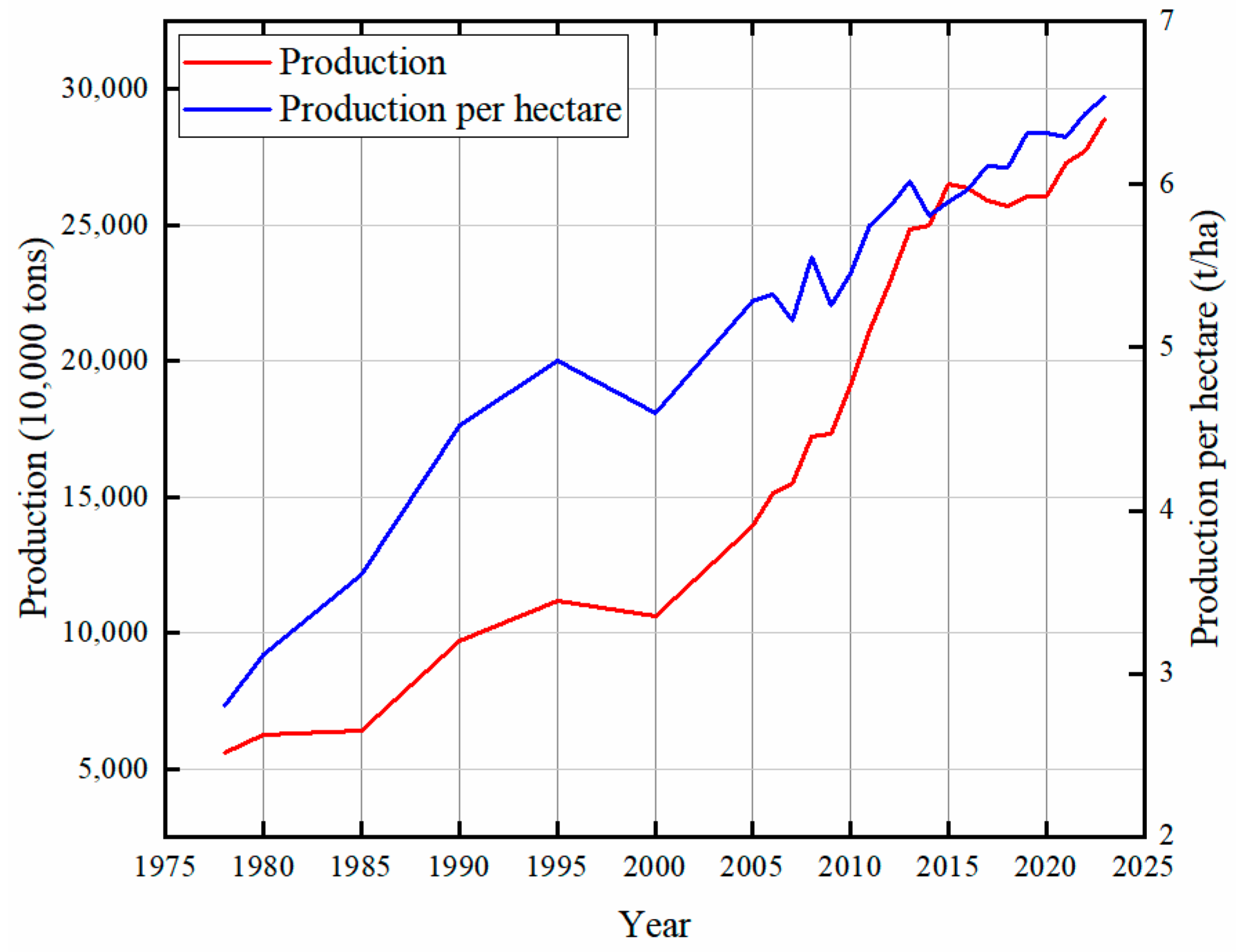
Maize is one of the top three worldwidely agricultural products, with a total production that ranks high among worldwide food crops. It is widely planted and currently one of the most extensively distributed crops in the world. In comparison to traditional food crops like wheat and rice, maize can adapt to most environments and has superior nutritional value [1]. Maize is also a very important feed crop, containing a variety of nutrients needed by poultry and livestock, and is a major source of feed for animal husbandry. At present, maize can be processed into starch, fermented products, alcohol, maize oil, maize food, maize plastics, and dozens of other types, as many as thousands of products, which are widely used in the food, aquaculture, chemical, medical, fuel, paper, textile, and other industries. According to the 2019–2023 yearbook of the National Bureau of Statistics of China, the average sown area of maize in China is 42.632 million hectares, accounting for 181 percent of the sown area of wheat and 144 percent of the sown area of rice. In 2023, China produced 272,200,200 tons of maize, which was twice of the total wheat production and 1.3 times of the total rice production (Figure 1). The advancement of the maize industry in China has a dual benefit: it enhances food security and fosters economic resilience. Furthermore, it uplifts rural livelihoods and supports broader economic goals [2].

Maize is a dietary staple for a significant proportion of the global population, and the successful cultivation of this crop is closely linked to the quality of the seeds used. Key indicators for assessing maize seed quality include moisture content, viability, maturity, and the presence of surface defects. These factors play a critical role in ensuring optimal growth and yield. Seed mildew has an important effect on maize vitality. Screening maize seeds before sowing is beneficial for increasing yield and income. During the storage period of maize seeds, according to their respiratory characteristics, with the increase in storage time, their respiratory intensity will continue to increase and continue to generate heat. The structural characteristics of the maize seed itself ensure that it is easy for endosperms rich in starch to inhale moisture and heat in the environment, thus becoming the most suitable growth environment for mold. If the storage conditions are not good, the mold in the environment will easily lead to more mold in high-moisture maize seeds produced by respiration and produce maize seeds with different degrees of mold [3]. If moldy seeds are not screened, moldy seeds will increase the rate of mildew in other seeds and reduce storage time. In addition, in moldy maize seeds, with the proliferation of microorganisms, many toxic mycotoxins will be metabolized, such as aflatoxin, zearalenone, etc. The impact of these mycotoxins on the growth and development of poultry and livestock is significant. In addition to damaging tissue and organ function, they can cause disease or death in affected animals. Furthermore, they can facilitate the transmission and prevalence of diseases by enabling the cross-infection and propagation of microorganisms. Moreover, the germination rate, seedling rate, and disease resistance of maize will decline markedly as a consequence of the presence of impurities in the seeds, which will consequently impact yield and the income of farmers [4]. Therefore, accurately classifying and identifying seed quality have become urgent problems to be solved. Consequently, in examining the detection of maize seed surface mildew, scientists and researchers may pursue a variety of strategies and techniques with the objectives of minimizing environmental impact and facilitating the advancement of sustainable agricultural practices.

Presently, the quality of crop seeds is still predominantly determined by traditional manual screening methods. These methods rely on the sensory system of operators, including the assessment of attributes such as touch, sight, and smell, in conjunction with personal experience, to evaluate quality. However, this method has many limitations, such as the insufficient consistency of the results, low efficiency, potential damage, and susceptibility to subjective bias, which means that it cannot fully and objectively reflect the true state of seeds. Especially in the detection of large quantities of samples, it is difficult for manual methods to meet the needs of modern agricultural production. In addition, while chemical sampling is an accurate method, it is both time-consuming and costly, making it unsuitable for large-scale commercial seed detection. The advancement of science and technology has led to the gradual integration of non-destructive testing techniques, including electronic nose technology, spectral imaging technology, image processing technology, and machine vision, into the domain of agricultural product testing. These methodologies offer robust technical support for the advancement of agricultural automation, reduce labor costs, and enhance detection efficiency and accuracy. The rise of computer vision technology has further promoted the development of image processing and gradually replaced manual operation. However, traditional computer vision relies on a lot of engineering experience and prior knowledge and analyzes image features by manually extracting them, which has limitations when dealing with complex problems. In contrast, machine learning (ML) techniques, particularly deep learning (DL), demonstrate enhanced adaptability and accuracy through the automatic learning of features within data sets. DL has demonstrated considerable success in a range of tasks, including image classification, localization, detection, segmentation, and tracking. The model multilayered architecture facilitates the learning of intricate feature representations, thereby enhancing the efficiency and precision of data representation learning. Applying DL to machine vision for processing and analyzing images of seeds can quickly and effectively detect mildew, improving seed quality, reducing the introduction of mold, ensuring food safety, and contributing to the modernization and automation of agricultural production. Although DL has demonstrated great potential in many fields, its application in agricultural crop detection still needs further research and exploration. This study aims to utilize DL algorithms to achieve the automatic detection of surface defects in maize seeds, enhancing seed quality, increasing germination rates, boosting yield and income, reducing labor costs, and providing strong support for agricultural production.

DL has been employed extensively in agricultural contexts. Yuan et al. proposed a novel type of point-centered convolutional neural network (CNN) that demonstrated superior performance compared to full-band-based CNNs and holds significant promise for the non-destructive identification of moldy peanuts [5]. Chen et al. integrated a near-infrared (NIR) snapshot hyperspectral sensor with DL to develop a multi-modal, real-time coffee bean defect detection algorithm for sorting defective green coffee beans [6]. Xuan et al. proposed a Partial Least Squares Discriminant Analysis (PLS-DA) model that uses spectral features for early diagnosis, which can effectively detect whether wheat leaves are infected with powdery mildew [7]. Lv et al. proposed an improved YOLOv5 algorithm and proposed a Bidirectional Feature Pyramid Network (BiFPN)-S structure, called the YOLOv5-B algorithm, which can accurately identify apple fruit growth in real time [8]. Zhang et al. combined the DL algorithm with edge detection threshold processing based on the optimized S2Anet (Single-shot Alignment Network) model, and the optimized algorithm was able to identify cracked and non-cracked seeds effectively [9].

The majority of current research in the field of maize crop detection is concentrated on the identification of defects and the classification of maize varieties. There is a paucity of studies addressing the detection of maize mildew. Javanmardi et al. proposed a new method using a deep CNN as a general feature extractor. Compared with the model based only on simple features, the model trained by extracting features using a CNN had a higher classification accuracy for maize seed varieties. A CNN–artificial neural network (ANN) classifier performed the best [10]. Wang et al. combined a dual-path CNN model to establish a defect detection method based on a watershed algorithm. The results proved that the model was effective in identifying defective seeds and defect-free seeds [11]. Suarez Patricia L et al. proposed a method for segmenting and classifying maize kernels, which solved the problem of inspecting the quality of maize seeds [12]. Song et al. proposed an improved seed quality evaluation method based on maize seeds with different qualities based on the Inception–Residuals Network (ResNet). The results showed that the proposed method had good comprehensive performance in the detection of maize seed appearance quality [13]. Liu et al. proposed an improved CST-YOLOv5s (YOLOv5s + CBAM + SPPCPSC + Transformer) algorithm, which was capable of detecting damaged and mildewed corn grains with high Precision and mAP50 value. However, the size of the model was increased to 1.93 times that of the original model [14]. In order to develop a portable device for the accurate detection of corn mildew, a new detection algorithm for corn mildew is urgently needed.

A review of the current research status at home and abroad reveals a plethora of studies on the quality of maize appearance varieties. However, there is a paucity of experiments on the detection of maize mildew. The focus of this study is to use DL technology to detect maize seed surface mildew. DL frameworks such as YOLOv5 were used to detect the surface defects of maize seeds, especially to identify healthy, mildly moldy, and severely moldy maize grains using self-created maize seed data sets. In order to achieve the above main goals, three aspects of work need to be completed: (1) The construction of a maize seed surface mildew detection hardware system. In accordance with the specifications for the detection of maize seed surface mildew, an image acquisition apparatus for maize seed surface mildew was devised, and a hardware system for maize seed surface mildew was assembled. The image data of healthy, mildly infected, and severely infected maize kernels were collected. (2) The process of data cleaning and image preprocessing. In order to meet the requirements of the DL algorithm with respect to both the image and data set, OpenCV was employed for the purpose of image preprocessing. Furthermore, the data set was augmented through a series of operations, including image transformation, enhancement, segmentation, filtering, and morphological processing, with the objective of enhancing the robustness of the trained model. (3) A DL algorithm for analyzing and detecting the collected data. According to the characteristics of maize seed surface mildew, a YOLOv5s model was used for training. On this basis, the YOLOv5s–Shufflenet model was proposed to replace the YOLOv5s backbone network with a ShuffleNet CNN. Then, a CBAM was integrated into the improved YOLOv5s–ShuffleNet neck network, resulting in the proposed YOLOv5s–ShuffleNet–CBAM model. Finally, a healthy maize kernel, slightly mildewed maize kernel, and severely mildewed maize kernel were identified, and the model volume was simplified [15].

2. Materials and Methods

2.1. Sample Preparation and Mildew Test

The objective of this study was to identify and differentiate between healthy and moldy grains in maize seeds. It is essential to obtain a substantial quantity of maize seeds exhibiting optimal visual characteristics, including the absence of mildew, for the purposes of model training and detection. The primary cause of maize seed mildew is a fungal infection, including, but not limited to, Aflatoxin, Aspergillus niger, Streptomyces griseus, Penicillium, etc. The seeds need to be infected with fungi in advance to meet the requirements, and pictures of the seeds at various stages of mildewing were taken. There are a lot of nutrients stored inside maize, which can be well preserved at 12.5% water content, but when the water content is 15%, mold may grow and multiply. With the increase in water content, the probability of mold also increases. When the water content is 45% to 60%, the maize itself will germinate. In order to simulate the actual environment of maize storage in a warehouse, the maize samples were dried to meet the storage requirements, and then the mildew experiment was carried out.

The species of Zhengdan 958 maize seed has the advantages of having a stable yield and high yield, strong adaptability, and wide planting area, and it is widely planted in China. Therefore, Zhengdan 958 kernels were used for the fungal infection experiment. During the experiment, Aspergillus niger, Penicillium, Aspergillus flavus, and other molds were inoculated to ensure mildew formation, while external bacteria were introduced to ensure the diversity of mold species. The experimental environment was set to a constant temperature of 23 °C and in a humidity chamber of 40%. In order to maintain the diversity of samples, maize samples were divided into 6 batches, and 300 maize seeds were taken out every 7 days for treatment, and the phenomena of mold infection were observed by taking photos. After obtaining a large number of sample data, the experimental data were divided and calibrated.

2.2. Image Acquisition System

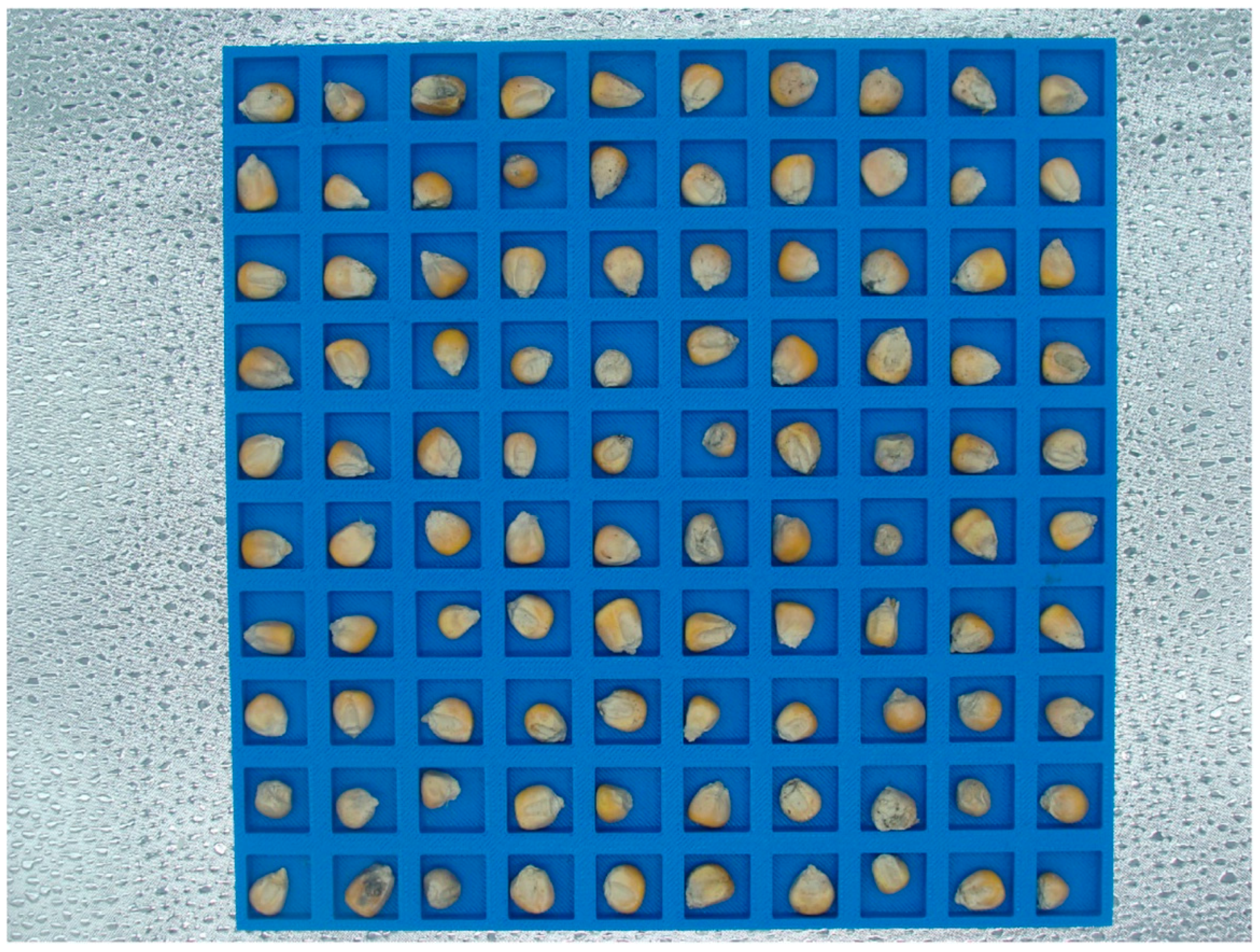
In order to obtain the surface mildew images of maize seeds, a maize seed detection platform was designed according to the existing conditions of the laboratory (Figure 2).

The system primarily consisted of a digital camera (DSC-H10, SONY, Tokyo, Japan) with an 8-megapixel sensor with 8.1 million effective pixels and a maximum of 8.3 million pixels. The camera supports a maximum resolution of 3264 × 2448 and USB 2.0 connectivity. It was mounted on a platform 500 mm above the detection platform to ensure stable image capture. The inspection platform was modeled using SolidWorks 2021 (Dassault Systemes, Waltham, MA, USA) and a 3D printer (Aurora A6 Industrial, Aurora Innovation, Shenzhen, China). The platform measures 200 × 200 × 7 mm (Length × Width × Height) and contains 100 grooves arranged in a 10 × 10 grid. Based on the initial measurements of the maize seeds, the grooves were designed with dimensions of 15 × 15 × 6 mm (Length × Width × Height), with a 5 mm spacing between adjacent grooves.

The quality of an image is of great consequence to the training of the model; the quality of the light source is similarly a significant factor affecting the quality of the data set and subsequent experiments. The light source was used to provide an environment conducive to achieving the desired imaging effect of the target, increasing the brightness of the environment and the target itself. Two LED strips with a size of 365 × 45 mm (Length × Width) and a power of 37.2 W were used. The LED strips were protected by a three-dimensional aluminum housing, and the angle of the light source could be adjusted by rotating slots on both sides of the strips. The adjustment results are shown in Figure 2b. A LED dimming studio with a size of 400 × 400 × 400 mm (Length × Width × Height) was used as a light source obscura (Figure 2a). This can guarantee the closure of the collection environment, prevent the interference of natural light and other stray light, and ensure the uniformity of lighting. A total of 100 maize seeds were imaged at a time, with all seeds positioned on the detection platform. The camera was situated in a fixed position to obtain images of the maize seeds through a designated aperture at the summit of the light source box. Subsequently, the captured images were transferred to a personal computer (PC) via a USB cable for further analysis and processing.

2.3. Imaging Processing

2.3.1. Image Preprocessing and Image Enhancement

The image segmentation algorithm based on the threshold value was adopted in this paper. The overall steps were divided into 8 parts: grayscale image processing, median filter denoising, image binarization, open operation, close operation, connected domain extraction, mark extraction, and image segmentation. Grayscale image processing is a fundamental operation that forms the basis for a number of subsequent image processing operations. The images captured by the acquisition system were initially represented in RGB format. Subsequently, OpenCV converts the images to BGR format and then transforms them to grayscale.

From the images provided (Figure 3), the details of the maize kernel appearance remained clearly visible, allowing for an accurate observation of its surface characteristics. However, owing to environmental conditions and hardware accuracy limitations, there were some noises in the image, which showed the contrast and overall quality of the image. In order to enhance this phenomenon, image enhancement technology was used as a requisite processing step. This technology serves to augment the visual impact of the image, thereby accentuating the information pertinent to the observer. By using image enhancement techniques, it is possible to reduce noise interference while maintaining the integrity of the original data. This allows the contrast and distribution of the images to be improved, thereby enhancing the readability of the maize kernels within the image. In the context of image enhancement, image filtering represents a common technique [16]. Mean filtering can smooth an image by calculating the average value of the pixel neighborhood but may blur the details while removing noise. Median filtering is a nonlinear filtering method based on ranking statistical theory, which is particularly well suited for the removal of salt-and-pepper noise. By selecting a window containing the target pixel and its neighboring pixels, the pixel values within the window are sorted, and the middle value is taken as the new value of the target pixel. This effectively removes isolated noise points. The Gaussian filter can use the Gaussian function as the convolution kernel and assigns different weights according to the distance between the pixel and the center pixel to achieve image smoothing. After comparing the effects of different filtering methods, we found that median filtering performed the best in removing salt-and-pepper noise from maize kernel images, significantly reducing the number of white dots in the images. Accordingly, median filter technology was selected for the purpose of reducing image noise processing, which has the potential to effectively suppress noise, enhance the clarity of maize kernels in the image, and provide a more robust foundation for subsequent image recognition.

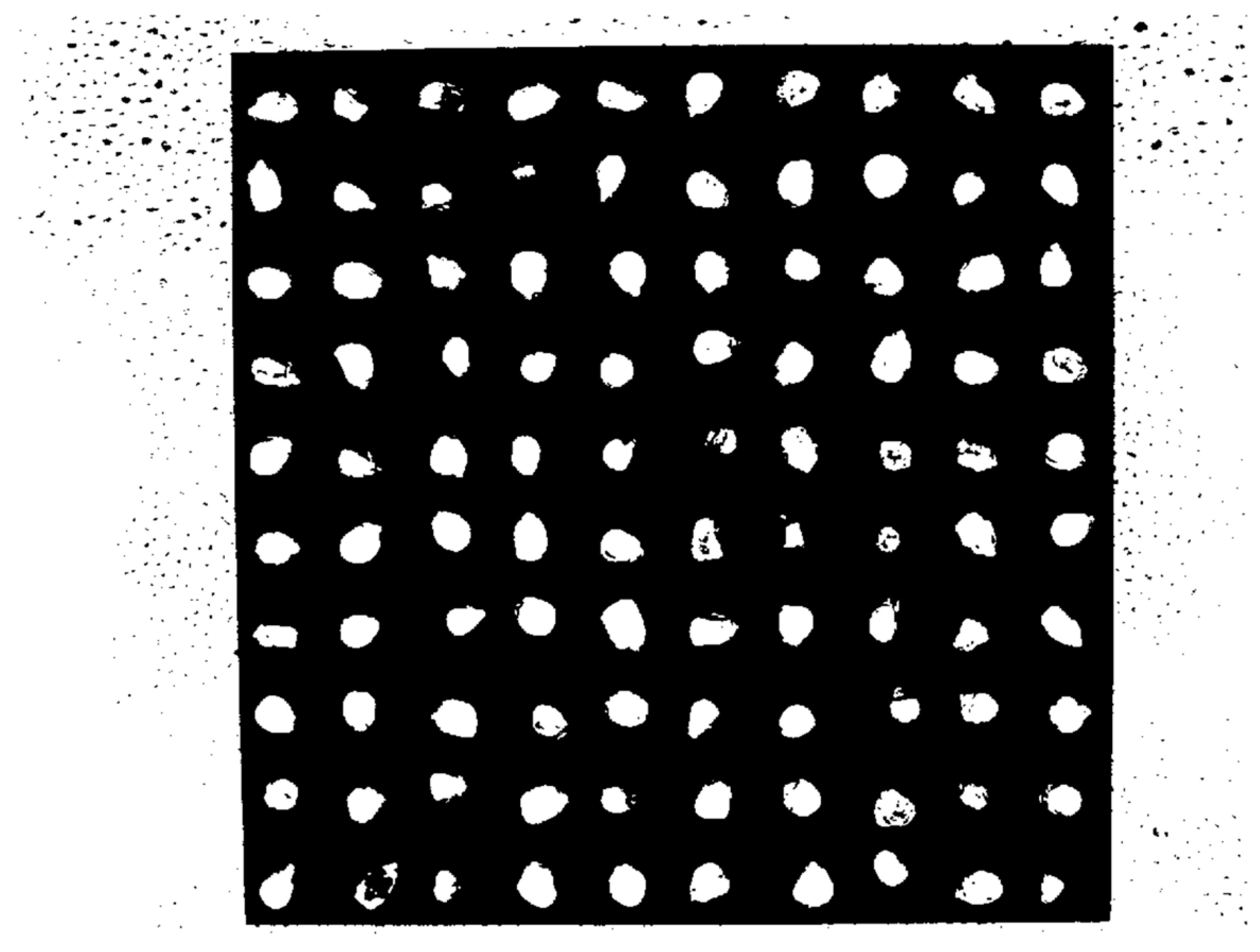
Following the application of a filtering technique to reduce noise, the Otsu binary image algorithm was employed to transform the image into a binary representation [17]. The method is uncomplicated and reliable, rendering it one of the most efficacious techniques for determining thresholds for image segmentation. As illustrated in Figure 4, the Otsu method resulted in the retention of numerous minor noises within the image, as well as the division of several maize kernels into multiple segments. To circumvent this problem, the image used open and close operations on several occasions.

In image processing, open operation and close operation are two important morphological operations [18]. The open operation first carries out the corrosion operation, followed by the expansion operation, utilizing the same structural elements. The etching operation can effectively remove the edge pixels of the image and smooth the outline of the object, but usually, the number of edge pixels removed is small. The expansion operation can fill small holes inside the object, connect the neighboring object, and also smooth the boundary of the object. By using the open operation, the object outline of the image can be smoothed, long and thin curves will be broken, and small protrusions can be eliminated, which can help eliminate noise and isolate pixels in the image. In contrast to the open operation, the closed operation first performs the expansion operation, followed by the corrosion operation, again using the same structural elements. The closing operation can make up for the narrow break curve in the image, eliminate small holes, and fill the break in the contour line, which can also help connect broken objects and recover details that may have been lost due to filming or processing.

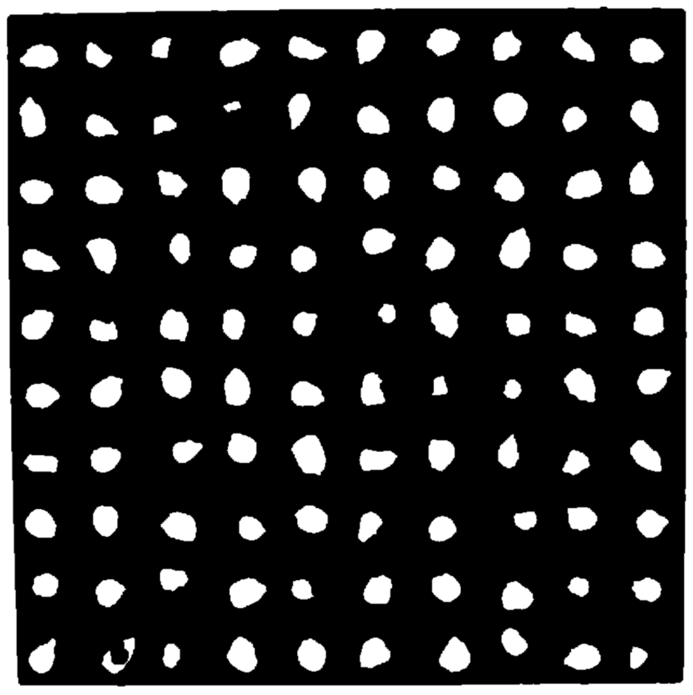
Following the application of open and close operations, it became evident that the isolated minor points surrounding the stage were eradicated, and the initially divided maize particles were reunified. This processing effect was very useful in image analysis, which could obviously improve the quality of the image and the accuracy of subsequent processing (Figure 5). As illustrated in Figure 4, the images were grouped together following the completion of the open and close operations. Despite the Otsu algorithm dividing the maize seeds into disparate sections, the open and close operations were still able to reunite them, effectively removing noise pixels while simultaneously rectifying image defects.

When processing maize images for accurate cutting, the minimum external rectangle method was adopted in this study. This method is a classical computational geometry technique that aims to determine the smallest rectangle that can tightly surround a specific area in an image, such as a maize seed. By applying the minimum external rectangle method, we were able to accurately locate the central point of the maize and obtain the coordinates of its four vertices, thus achieving an efficient division of the maize seeds (Figure 6). In order to ensure the integrity of each kernel image and adapt to the processing requirements of the subsequent network model, a certain number of pixels were expanded from the initial minimum external rectangle. This step was conducted to avoid losing any important features or details of the maize seed during cropping, thus ensuring that the resulting single-case maize seed image was complete and suitable for further analysis. By this method, the image of a single maize seed could be effectively extracted from the original image to provide a high-quality data set for the subsequent processing and recognition.

2.3.2. Data Annotation

In this study, the YOLOv5s DL framework used the LabelImg annotation tool to annotate and classify the data set. The maize seeds were categorized and numbered accordingly. Just to make sure that we set all samples on the same page with the molding process, we took out a batch of maize every week to process into images. We cut seeds into three images, with 100 maize seeds in each. We divided the samples into three groups: the Train (samples 1–60), the Test (samples 61–80), and the Val (samples 81–100). We ended up with six batches of seeds, with a total of 1800 images. We ended up with 1080 train images, 360 validation images, and 360 test images. This partitioning method ensured consistency in the timing of mold development among the training, validation, and test sets, minimizing errors. The maize seeds were classified according to their visual characteristics. Seeds exhibiting optimal health and appearance were designated as “Sound”, while those displaying slight mold growth were classified as “Mild”, and those with severe mold infestation were designated as “Severe”. This classification system was utilized for the final model performance evaluation. The individual maize seeds were then subjected to segmentation, and the resulting data set is presented in

Table 1. Sample numbers of maize data set.

Class	Train	Val	Test	Total
Sound	274	112	105	491
Mild	534	152	171	857
Severe	272	96	84	452

. We did not use oversampling or loss re-weighting. The focus of our study was the early mildewing of maize seeds. The characteristics of severe maize are easily discernible, whereas the mild maize forms of the disease are more difficult to identify. Additionally, in real-world scenarios, the prevalence and meaning of maize exhibiting only early mild symptoms are significantly higher than those of maize with severe symptoms. This makes the detection of early-stage disease in maize a highly practical objective. Consequently, our study incorporated a greater proportion of corn exhibiting only early mild symptoms.

2.4. Evolution and Advantages of DL in Object Detection

The DL algorithm can overcome feature subjectivity in the feature extraction method of the traditional algorithm and improve the universality of model application scenarios. In particular, the application of CNNs can not only significantly improve the accuracy of detection but also make a qualitative leap in processing speed and efficiency [19]. CNNs are DL models that belong to a branch of ANN. In the field of computer vision, CNNs are widely used in image classification, image generation, target detection, and other tasks and have achieved good results. The application of CNNs in the field of object detection marks a major revolution in the field of DL.

CNNs comprise several layers, including the input layer, convolutional layer, pooling layer, activation layer, and fully connected layer. By using local perception, weight sharing, and spatial context, they can effectively extract image features. The advantages of CNNs include the following: The use of convolutional layers and pooling layers to extract local image features reduces the number of model parameters and the amount of calculation, thereby reducing the complexity and degree of overfitting in the model and optimizing it. Moreover, CNNs can better extract all kinds of features in image processing and improve the robustness of the model. It is generally believed that in the past 20 years, target detection has experienced two stages: The first is that of the traditional target detection method before 2014. In the second, in the period of object detection based on DL after 2014, there are two major branches, i.e., the CNN represented by Faster R-CNN and the single-stage object detection algorithm represented by YOLO.

Two-stage object detection algorithms usually include two main stages. The first stage is the generation of candidate target regions, usually through a Region Proposal Network (RPN) or other methods. The second stage consists of classifying and refining these candidate regions. Two-stage algorithms generally excel in the accuracy of target detection tasks. They can provide high-quality target detection results and are especially suitable for complex scenarios and applications requiring high precision. However, due to the need for two independent phases, two-phase algorithms generally require more computational resources and time. As a result, their reasoning speed is relatively slow.

3. Results and Discussion

3.1. Surface Mildew Detection of Maize Seeds Based on YOLOv5s

With the continuous progress of target detection technology, the YOLO series, as a representative of single target detection methods, has made remarkable achievements in the field of real-time target detection by virtue of its unique design concept and superior performance. The single-stage target detection algorithm completes the target detection task in a single forward propagation without generating candidate regions. This algorithm can predict the category and location of the target directly through a dense grid or anchor box. Single-stage algorithms usually have faster inference speed and are suitable for real-time applications or scenarios with high-speed requirements. While single-stage algorithms have advantages in terms of speed, they are generally slightly less accurate than two-stage algorithms. However, some advanced single-stage algorithms have made significant progress in accuracy [20].

As the fifth version of the YOLO algorithm, YOLOv5 has made many innovations and improvements on the basis of the previous version and is also widely used in the current single target detection algorithm, with relatively high accuracy and detection speed. At present, YOLOv5 has five network structures: YOLOv5s, YOLOv5m, YOLOv5l, YOLOv5x, and YOLOv5n. The traditional YOLOv5 algorithm is mainly composed of input, backbone, neck, and head networks [21]. In this study, maize seed surface mildew detection was conducted using YOLOv5s, a lightweight version of the YOLOv5 series. The YOLOv5s model was trained specifically for this task.

3.2. ShuffleNetV2 Convolutional Neural Network

ShuffleNetV2 is a deep neural network architecture for efficient and accurate object recognition tasks. The network model was proposed in 2018 and proved to be more accurate than ShuffleNetV1 and MobileNetV1 at the same complexity [22]. The main role of ShuffleNetV2 is to reduce the computational cost of CNNs while maintaining high accuracy, and it achieves this by using a novel channel shuffle operation and a packet convolutional strategy. Channel shuffle operation is designed to exchange information between different channel groups. By mixing channels, ShuffleNet facilitates the flow of information across groups, helping to reduce parameters and computation without losing performance [23]. The packet convolution strategy divides the input channels into multiple groups, and convolution operations are performed separately within each group. This approach further reduces computational costs by reducing the number of connections and computations within the convolution layer.

The researcher points out that floating point operations per second (FLOPs) can only be used to evaluate the complexity of the model theoretically in current studies; instead of only being used as an evaluation criterion to judge the quality of the model, it should also start from the actual reasoning speed of the model and put forward four criteria for building the model: (1) The output and input channels of the convolutional channel layer should be consistent so that the memory consumption is minimal and the running speed is the fastest. (2) The convolution of the number of convolution groups should not be too large. Otherwise, the performance will be affected. (3) Reducing the number of network branches will improve the running speed of the model. (4) The influence of element-level operations on network speed cannot be ignored. Based on the above four criteria, this researcher designed the ShuffleNetV2 network model.

The ShuffleNetV2 model has a new and lighter basic unit. The basic block consists of two different structures; as shown in Figure 7, one is a structure with a stride of 1; another is a structure with a stride of 2. The main branches of these two structures are composed of three convolution layers, namely, 1 × 1 ordinary convolution, 3 × 3 depth separable convolution, and 1 × 1 ordinary convolution. But the composition of the input and side branches is different. In the structure with step size 1, the input side performs channel segmentation, and the side branch directly splices the channel segmentation image with the main branch image in dimension. In the structure with step size 2, the image is directly entered into the input end and processed by two branches, whose side branches are composed of 3 × 3 depth separable convolution and 1 × 1 ordinary convolution. In these two structures, the information communication between the two branches can finally be carried out through channel mixing.

3.3. CBAM: Convolutional Block Attention Module

CBAMs combine spatial attention mechanisms and channel attention mechanisms to overcome the limitations of traditional CNNs in processing information of different scales, shapes, and directions [24]. Compared with the traditional channel attention mechanism, the CBAM pays special attention to the sequential relationship between feature graph channels. At the spatial level, the CBAM enables the neural network to focus on the pixel regions in the image that play a decisive role in the classification result while focusing less on regions that contribute to the classification. At the channel level, the CBAM is used to process the weight distribution between the feature graph channels to ensure that the model can effectively use the information of different channels. The CBAM significantly improves model performance when applied simultaneously at both the spatial and channel levels. Compared with the SE (Squeeze-and-Excitation) attention mechanism, the CBAM attention mechanism not only adopts average pooling but also adopts maximum pooling, which reduces the information loss caused by pooling to a certain extent, making the CBAM more advantageous when dealing with complex problems [25].

As shown in Figure 8, the CBAM attention mechanism first conducts a global maximum pooled downsampling and a global average pooled downsampling for input feature $\mathit{F}$, and $\mathit{F}$ changes from the original $H\times W\times C$ to two $1\times 1\times C$ feature maps, and then these two feature maps are input into the fully connected multilayer perceptron, and finally, two $1\times 1\times C$ feature maps are output. After obtaining these two feature maps, the sigmoid activation function is used to limit the maps’ amplitude between 0 and 1, which is the same as that in channel attention, i.e., ${\mathit{M}}_{\mathit{c}}$ in the figure; the size is $1\times 1\times C$, and the formula is as follows:

$${\mathit{M}}_{\mathit{c}}(\mathit{F})=\sigma (MLP(Avgpool(\mathit{F})+MLP(Maxpool(\mathit{F})))$$

(1)

After the feature graph ${\mathit{M}}_{\mathit{c}}$ is obtained, it is not directly input into the spatial attention mechanism, but the feature graph ${\mathit{F}}_{\mathit{c}}$ is obtained by multiplying $\mathit{F}$ and ${\mathit{M}}_{\mathit{c}}$. The size of ${\mathit{F}}_{\mathit{c}}$ is the same as $\mathit{F}$, both of which are $H\times W\times C$. Then, the spatial attention mechanism obtains an $H\times W\times 2$ feature graph through a global maximum pooling subsampling and a global average pooling subsampling and then obtains an $H\times W\times 1$ feature graph through a convolution and finally limits its amplitude between 0 and 1 through a sigmoid activation function to obtain the final ${\mathit{M}}_{\mathit{s}}$. Its dimensions are $H\times W\times 1$. Finally, the resulting ${\mathit{F}}_{\mathit{c}}$ is multiplied by ${\mathit{M}}_{\mathit{s}}$ to obtain the final output feature ${\mathit{F}}_{\mathit{c}\mathit{s}}$, the size of which is also H × W × C.

$${\mathit{M}}_{\mathit{s}}(\mathit{F})=\sigma (f^{7\times 7}(Avgpool(\mathit{F})+MLP(Maxpool(\mathrm{F})))$$

(2)

where ${\mathrm{ƒ}}^{7\times 7}$ represents the convolution kernel of 7 × 7.

3.4. Replacement of Model Backbone Networks and Addition of Attention Mechanisms

The initial step is to register the ShuffleNet module in the ‘common.py’ file. Subsequently, the module is incorporated into the ‘yol.py’ file. A duplicate of the YOLOv5 configuration file, designated “YOLOv5s-ShuffleNet”, was generated, and the underlying network was substituted. The replacement YOLOv5s–ShuffleNet model comprised 193 layers and 849,882 parameters. In comparison to the direct application of the YOLOv5s model, while the number of layers exhibited a slight increase, the number of parameters was merely 12% of that of the original model.

Subsequently, the “YOLOv5s-Shufflenet-CBAM” configuration file was generated based on the “YOLOv5s-ShuffleNet” model, resulting in the final model. Figure 9 shows the YOLOv5s-Shufflenet-CBAM network framework. In comparison to the original model, this model comprises 221 layers and 1,066,428 parameters. It is slightly superior to the “YOLOv5s-ShuffleNet” model, exhibiting a 15.2% improvement.

In the context of CNNs, the number of parameters has a direct impact on computational speed, as it represents the number of parameters that the network must calculate. Reducing the number of parameters significantly improves the network computational speed. In terms of memory consumption, memory resources are crucial. During training, a large number of parameters require the network to store weights and intermediate states, which places a high demand on storage space. This is of particular importance for embedded or mobile devices, where memory limitations can impact the viability of the model for implementation. Furthermore, the number of parameters affects the model complexity and expressiveness. Incorporating additional parameters can improve the model ability to learn, but it can also lead to overfitting, which reduces the model accuracy. In conclusion, the substitution of the YOLOv5s backbone with ShuffleNet–CBAM results in a notable reduction in the number of parameters, thereby reducing both the computational and memory requirements. This renders it an optimal choice for deployment on embedded or mobile devices.

3.5. Model Parameter Selection and Training for Recognition

In this study, the computer utilized an Intel^® Xeon^® Platinum 8352V central processing unit (CPU) with a frequency of 2.10 gigahertz (GHz) and an NVIDIA^® RTX 4090 graphical processing unit (GPU). The operating system utilized was Ubuntu 20.04, and the programming language employed was Python 3.8. The deep learning frameworks employed were PyTorch 1.10.0 and CUDA 11.3. The network parameter settings employed the stochastic gradient descent (SGD) loss minimization algorithm, with a batch size of 16. This entailed the random selection of four images and their corresponding labels from the input images per batch for training purposes. The learning rate was set to 0.01, with a learning rate decay factor of 0.001, and the momentum parameter was configured to 0.937. The improved model completed 1000 training epochs.

3.6. Model Evaluation Metrics

In this study, the performance of the model in detecting maize seed surface mildew was evaluated from the following aspects:

(1) Precision refers to the proportion of true positive predictions out of all the instances that were predicted as positive. The formula is as follows:

$$Precision={\displaystyle \frac{TP}{TP+FP}}$$

(3)

where True Positives (TP) refer to instances where the model correctly predicts the positive class. False Positives (FP) refer to instances where the model incorrectly predicts the positive class.

(2) $Recall$ measures the proportion of actual positive cases that the model correctly identifies.

$$Recall={\displaystyle \frac{TP}{TP+FN}}$$

(4)

where False Negatives (FN) refer to instances where the model incorrectly predicts the negative class.

(3) $mAP\mathsf{50}$ provides an overall measure of a model precision and recall across different classes and Intersection over Union (IoU) thresholds. The formula is as follows:

$$mAP\mathsf{50}={\displaystyle \frac{T{P}_1+T{P}_2+\cdots T{P}_n}{T{P}_1+T{P}_2+\cdots T{P}_n+F{P}_1+F{P}_2+\cdots F{P}_n}}$$

(5)

where $T{P}_i$ represents the number of correct predictions for the $i$-th category, and $F{P}_i$ represents the number of incorrect predictions for the $i$-th category.

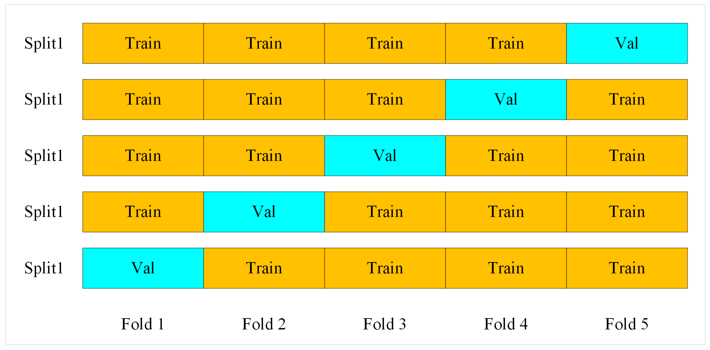
(4) Five-fold cross-validation is a pretty common method for assessing models. It helps improve a model generalization ability and reduce overfitting. To ensure the final model is stable, the following steps were applied: As shown in Figure 10, the entire data set was randomly divided into five distinct subsets. Subsequently, the models were trained and tested five times, with four parts of the data set utilized as the Train and the remaining part as the Val each time. Ultimately, the results were averaged to obtain the final evaluation.

3.7. Model Comparison Analysis

To ensure the final enhanced model meets the desired specifications, a series of experiments were conducted, and three lightweight model backbones (GhostNet, ShuffleNet, and MobileNet) were integrated into the YOLOv5s model. Concurrently, to address the diminution of feature values resulting from model lightweighting, three attention mechanisms were incorporated: the Shuffle Attention (SA), Coordinate Attention (CA), and CBAM mechanisms were employed.

As can be seen from

Table 2. Results of YOLOv5s model.

Class	Precision [%] ↑	Recall [%] ↑	mAP50 [%] ↑	Size (MB) ↓
YOLOv8s	86.7	90.9	95.9	21.48
YOLOv8s–ShuffleNet	89.6	90.7	96.3	12.45
YOLOv8s–ShuffleNet–CBAM	87.5	93.2	96.6	13.11
YOLOv5s	88.3	88.0	94.3	13.80
YOLOv5s–ShuffleNet	87.0	87.4	92.8	1.97
YOLOv5s–ShuffleNet–CBAM	90.2	88.0	95.5	2.40
YOLOv5s–MobileNet–CBAM	86.9	90.3	94.8	3.46
YOLOv5s–MobileNet–CA	87.3	88.1	93.6	3.05
YOLOv5s–MobileNet–SA	86.7	89.9	94.5	3.04
YOLOv5s–ShuffleNet–CA	86.8	85.5	92.9	1.99
YOLOv5s–GhostNet–CBAM	83.3	90.9	95.7	11.82

Note: (↑) means the higher value is better; (↓) means the lower value is better and the most accurate item are shown in bold.

, the YOLOv8s model outperforms YOLOv5s in terms of performance and mAP50. However, YOLOv8s has a larger size, which makes it too bulky for model lightweighting. Also, YOLOv5s can effectively improve the Precision, Recall, and mAP50 of model for the same model improvement, but YOLOv8s does not show the same performance improvement. In the final model, with the same improvement, we found that YOLOv5s–ShuffleNet–CBAM could obtain similar results to YOLOv8s–ShuffleNet–CBAM while being much smaller, so we decided not to choose the improved YOLOv8s model, but instead, the YOLOv5s was finally chosen.

Additionally, compared with the original model (YOLOv5s), the improved YOLOv5s models all have reduced model sizes compared to the original model, with the YOLOv5s–ShuffleNet–CA model being the smallest but not having a good improvement. While the YOLOv5s–MobileNet–CBAM model is the most balanced, the Recall and mAP50 values have a good improvement, and the model size is greatly reduced but not as significantly compared to other models. Meanwhile, YOLOv5s–ShuffleNet–CBAM has higher mAP50 values and has the highest Precision value and has a small model size. YOLOv5s–GhostNet–CBAM has the highest mAP50 value, but the model size is not significantly reduced.

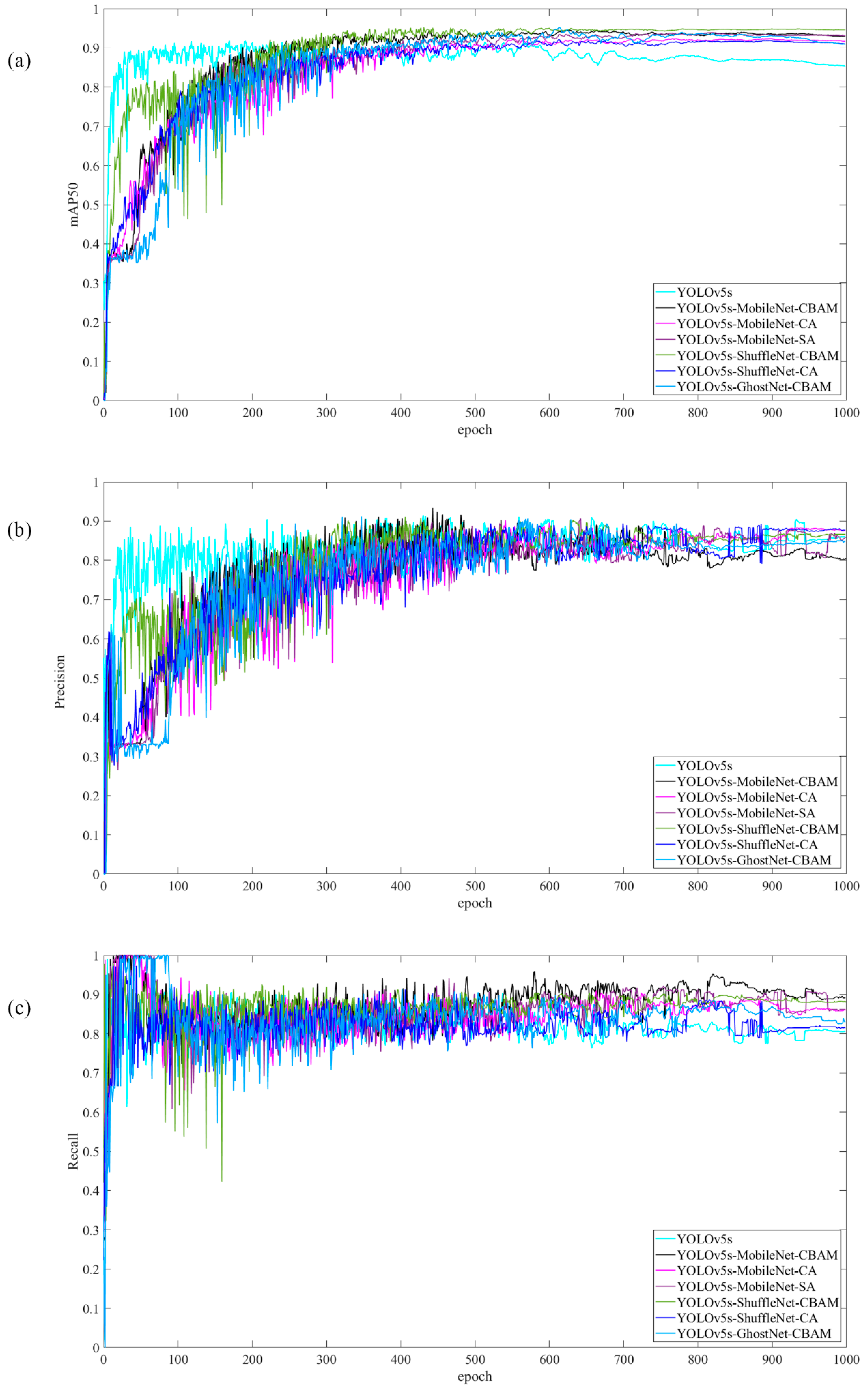
Also, through Figure 11, we could see that with 1000 rounds of training, the models YOLOv5s–MobileNet–CBAM, YOLOv5s–MobileNet–SA, YOLOv5s–ShuffleNet–CA, and YOLOv5s–GhostNet–CBAM had mAP50 values that eventually converged to 0.93, and considering a combination of model size and mAP50 values, we decided to choose the YOLOv5s–ShuffleNet–CBAM model as the final model. It can be seen that the YOLOv5s model finally stabilized at around 85%. The YOLOv5s–ShuffleNet–CBAM model was stable at 0.946, and the stability of the improved model was greatly improved [26].

Gradient-weighted Class Activation Mapping (Grad-CAM) is a powerful technique used to visualize the regions in an image that contribute the most to the predictions made by a CNN. This method helps in understanding how models make decisions, particularly in tasks like image classification and object detection. As shown in Figure 12, it was observed that Grad-CAM in the “Sound” seeds exhibited smooth isotherms. In contrast, the “Mild” and “Severe” seeds displayed irregular isotherms. The “Mild” seeds exhibited the presence of small black spots, whereas the “Severe” seeds displayed a predominantly deep red coloration. The Grad-CAM method proved to be an effective means of evaluating the reliability of the model, due to the distinctive features it exhibited.

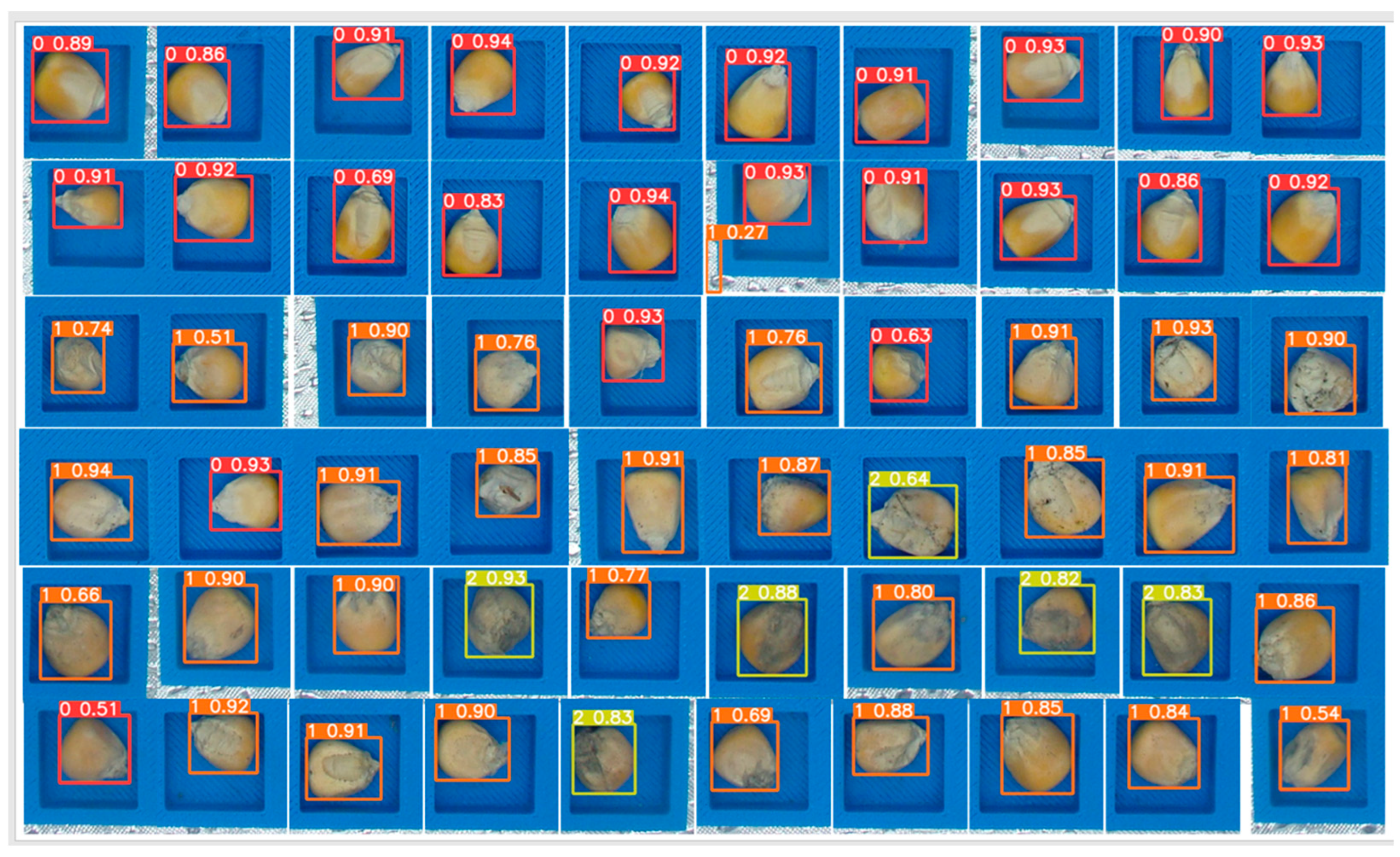
Figure 13 illustrates the detection results of the YOLOv5s–ShuffleNet–CBAM model for different degrees of maize Fusarium infection. It is evident that the model exhibits high precision in identifying healthy maize, and it is also capable of detecting minor fungal lesions that are often overlooked by human observers.

4. Conclusions

In this study, the improved YOLOv5s–ShuffleNet–CBAM model could greatly reduce the model size, fully meet the lightweight requirements, and lay a software foundation for the development and deployment of future mobile devices for the detection of maize seed surface mildew [27]. The improved YOLOv5s–ShuffleNet–CBAM model has the potential to markedly accelerate computational speed and reduce model size. In terms of evaluation indicators, compared with YOLOv5s, the improved YOLOv5s–ShuffleNet–CBAM model could not only have no loss in detection in Precision but also show improvement to a certain extent, with a Precision rate of 90.2%, a recall rate of 88.0%, and a mAP50 of 95.5%. Importantly, the model size was reduced from 13.8 MB to 2.4 MB with a decrease of 82.6%. The model performs similarly to the enhanced YOLOv8s model but with only 18.3% of the size. Additionally, the K-fold cross-validation proved the model stability, and Grad-CAM validated the model effectiveness. The improved model not only preserves its high degree of accuracy in identifying moldy maize seeds, but its overall complexity is also significantly reduced, thereby facilitating its deployment on a diverse range of platforms, including embedded devices, mobile devices, and online platforms within the specified application domain. In future work, a further refinement of the improved YOLOv5s–ShuffleNet–CBAM model will focus on ensuring a lightweight architecture while maintaining high precision, with the aim of enhancing practical applications and streamlining deployment in real-world scenarios.