Reconstructing High Dynamic Range Image from a Single Low Dynamic Range Image Using Histogram Learning ^†

Abstract

High dynamic range imaging is an important field in computer vision. Compared with general low dynamic range (LDR) images, high dynamic range (HDR) images represent a larger luminance range, making the images closer to the real scene. In this paper, we propose an approach for HDR image reconstruction from a single LDR image based on histogram learning. First, the dynamic range of an LDR image is expanded to an extended dynamic range (EDR) image. Then, histogram learning is established to predict the intensity distribution of an HDR image of the EDR image. Next, we use histogram matching to reallocate pixel intensities. The final HDR image is generated through regional adjustment using reinforcement learning. By decomposing low-frequency and high-frequency information, the proposed network can predict the lost high-frequency details while expanding the intensity ranges. We conduct the experiments based on HDR-Real and HDR-EYE datasets. The quantitative and qualitative evaluations have demonstrated the effectiveness of the proposed approach compared to the previous methods.

1. Introduction

As imaging technology advances, image quality has improved significantly over the past few decades. The ultimate goal is to present images of real scenes that are directly visible to the human eye. Although several aspects of visual sensing capabilities, such as image resolution, color accuracy, and optical sharpness, have been enriched, the luminance range of current imaging devices is still limited compared to the human visual system. This is mainly due to the adaptability of visual perception to large illumination changes, but photosensitive elements can only collect a fixed amount of light. Moreover, although high dynamic range (HDR) cameras can be used for directly capturing HDR images, they can still not cover the entire dynamic range of a scene. Therefore, it is essential to generate an HDR to increase the contrast of image content to achieve colorful scene representation.

The dynamic range of an image represents the ratio between the maximum and minimum measurable light intensities. Low dynamic range (LDR) images record 8 bits of information for each channel of each pixel. In general, it lacks sufficient quantization levels to cover wide intensity variations. The presented dynamic range is much lower than the real scene and cannot meet our needs for image visual effects.

Several approaches [1,2,3,4] have been proposed for reconstructing HDR images that can record richer light and dark changes. An image acquisition technique [1] is to take multiple images with different exposure values in the same scene, also called bracketed exposure images, and combine these images into an HDR image. Although this technique can effectively produce HDR images, it may be affected by scene changes in dynamic scenes, making it difficult to achieve desirable results. It is also limited by the difficulty in obtaining bracketed exposure images and cannot be directly applied to existing images. Several approaches [2,4] focused on solving the problem of object shaking and artifacts when shooting bracketed exposure images. However, the techniques of using multiple images are still inconvenient in data acquisition and application.

One way to generate an HDR is to extend a single LDR image to its HDR counterpart. The so-called LDR2HDR technique utilizes an inverse tone mapping operator to extend the dynamic range [5,6,7]. For the last decade, convolutional neural networks (CNNs) have been intensively studied in LDR2HDR algorithms [8,9]. These reconstruction approaches for HDR images have greatly improved their practicality and improved the problems of previous methods. However, reconstructing an HDR image from a single LDR image is always a challenging task.

In this paper, we propose a two-stage approach for reconstructing an HDR image from an LDR image using histogram learning. In the first stage, we first perform a preliminary dynamic range extension on the input LDR image to an extended dynamic range (EDR) image. Then, we use a neural network to learn the changes from EDR image histograms to HDR image histograms. Next, we predict an HDR histogram of the EDR image through cumulative histogram learning. Finally, we use the predicted HDR histogram to perform histogram matching on the EDR image to generate the first-stage HDR output image. In the second stage, the final HDR image is reconstructed using reinforcement learning with pixel-level rewards for local consistency adjustment. Hence, we can obtain favorable HDR image quality using the proposed approach. For applications, several vision systems require an HDR camera for capturing high-quality images including autonomous mobile robots, autonomous guided vehicles, smart traffic management systems, etc.

The contributions of the proposed approach are summarized below: (a) we propose an efficient two-stage LDR2HDR approach with histogram expansion and pixel allocation; (b) we introduce a histogram learning approach to predict the intensity distribution of a single LDR image; and (c) we use reinforcement learning to perform pixel-wise adjustments on histogram-matched HDR images.

2. Related Works

Several methods [5,7,8,10,11,12,13] have been intensively studied to extend a single LDR image to an HDR image. Lin and Kao [5] presented a bit slicing approach combined with stereo matching algorithms for HDR images reconstructed from multiple exposures. Their approach can achieve comparable bad pixel rates on stereo matching using only the most significant 16 bits of an HDR image encoding per pixel. This approach demonstrated desirable results compared to the previous methods. Rempel et al. [7] proposed a reverse tone mapping algorithm for reconstructing the HDR of videos and images from LDR contents for viewing on HDR displays. Their algorithm was efficient to work in real time and no user input was required. Moreover, this method did not produce disturbing artifacts and the visual quality of the HDR output image was good.

For learning-based approaches, Eilertsen et al. [10] proposed a fully convolutional hybrid dynamic range autoencoder to predict HDR values in saturated regions to recover the loss of detail. Their approach can predict information lost in saturated image areas to reconstruct an HDR image from a single LDR image. The results demonstrated that this approach can reconstruct visually convincing HDR results in a wide range of situations compared to existing methods. Santos et al. [12] presented a learning-based technique to reconstruct an HDR image by recovering the saturated pixels of an input LDR image. They proposed a feature masking mechanism to reduce the influences of saturated areas and adopted a perceptual loss function to synthesize images with visually pleasant textures. Their approach can address ambiguity during training, checkerboard, and halo artifacts. Inspired by the LDR image formation pipeline, Liu et al. [11] proposed a technique to reverse the steps of LDR image formation to gradually restore HDR images that are close to the real scene. This approach proposed to learn three specialized CNNs to reverse three steps including dynamic range clipping, non-linear mapping from a camera response function, and quantization. Alternatively, a data-driven learning method [14] was proposed to reconstruct information lost from the original image due to quantization, dynamic range cropping, tone mapping, or gamma correction. This technique reconstructed an HDR image from an LDR image using deep CNNs.

Lightweight deep neural network models have increasingly attracted much attention due to the demand for real-time processing capabilities. Wu et al. [13] proposed a lightweight CNN to reconstruct an HDR image from a single LDR image. They used up-sampling blocks in the decoder to alleviate artifacts while maintaining computational speed. Their approach can recover the lost information in saturated regions and reconstruct HDR images of high quality. Guo and Jiang [15] presented an approach to improve HDR reconstruction for legacy content through camera pipeline modeling. They proposed a lightweight deep neural network (DNN) for legacy standard dynamic range (SDR) images containing unreproducible historical scenes. The results showed that this approach can achieve appealing performance with minimal computational cost. Cao et al. [16] presented a brightness-adaptive model based on deep learning to produce an HDR image for one single LDR image. They proposed an inverse tone mapping model based on brightness adaptive kernel prediction. The LDR image was first convolved with an adaptive kernel and then reweighted to obtain HDR results. The results showed that this approach outperforms the previous methods. To simultaneously solve the image super-resolution problem, Kim et al. [17] proposed a joint image tone mapping and super-resolution framework using a multi-purpose CNN structure. This approach can reconstruct fine details by decomposing the input image and focusing on the low-frequency and high-frequency layers. Moreover, they applied location-variant operations to enhance local contrast. This approach can obtain good quality results with increased contrast and details.

3. Proposed Approach

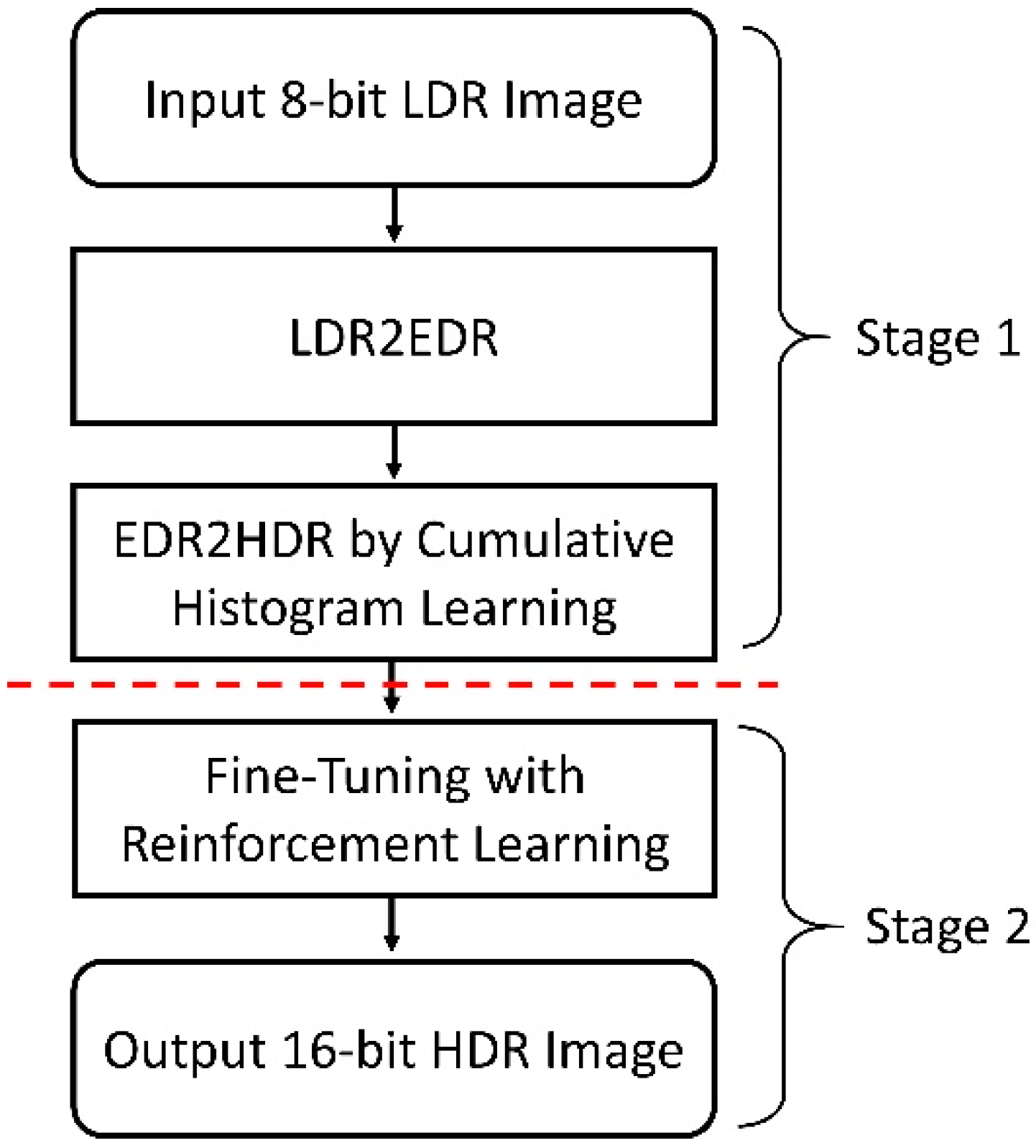
The flowchart of the proposed two-stage approach is shown in Figure 1. In the first stage, our approach first applies pixel multiplication, image upsampling, and downsampling to convert an input 8-bit LDR image into a 12-bit EDR image. For the EDR image, we calculate the cumulative distribution function (CDF) of the intensity histogram. Subsequently, to learn the intensity distribution of HDR images, 16-bit ground-truth HDR images are converted to their 12-bit representations and used as ground truths for EDR histogram reshaping. We use a deep neural network to learn the differences between cumulative histograms of EDR-HDR image pairs and thus predict target histograms of HDR images from EDR images. Using the prediction as a reference for histogram matching, we can obtain a 12-bit HDR image with intensity distribution updates. In the second stage, the obtained 12-bit HDR image is converted to a 16-bit HDR image with intensity scaling (multiplied by 2⁴). Then, reinforcement learning and pixel rewards are used to fine-tune intensity values for reconstructing the final 16-bit HDR image.

Figure 1. Flowchart of the proposed two-stage approach.

3.1. LDR2EDR

To produce a 12-bit EDR image from an 8-bit LDR image (LDR2EDR), we first multiply the intensity of each pixel by 2⁴. That is, the dynamic range extends from [0, 255] to [0, 4095]. To fill the empty bins in the histogram of the EDR image resulting from direct scaling, the image is upsampled using bicubic interpolation to obtain a continuous histogram distribution. The bicubic interpolation technique considers 2² × 2² pixels (16 samples) nearest to a new pixel to be determined and computes the new pixel value through the weighted average of the pixel values of these 16 samples. The weight of each sample is determined by the distance to the new pixel. We use the following interpolation weight kernel to perform the convolution operation.

$$W\left(i\right)=\left\{\begin{array}{c}\left(\alpha +2\right){\left|i\right|}^3-\left(\alpha +3\right){\left|i\right|}^2+1,\mathrm{for}\left|i\right|\le 1\\ \alpha {\left|i\right|}^3-5\alpha {\left|i\right|}^2+8\alpha \left|i\right|-4\alpha ,\mathrm{for}1<\left|i\right|<2\\ 0,\mathrm{otherwise}\end{array}\right..$$

(1)

where i denotes the generic sample, $\alpha$ is −0.5 or −0.75, and $\alpha$ determines the performance of the kernel. Note that W(0) = 1 and W(n) = 0 when n is a nonzero integer. The pixel intensity f(x, y) of the new image is then given by

$$f\left(x,y\right)={\sum }_{i=0}^3{\sum }_{j=0}^{3}f\left(x_i,y_j\right)W\left(x-x_i\right)W\left(y-y_j\right).$$

(2)

where $f(x,y)$ is the interpolation function, W is the interpolation kernel, and $f(x_i,y_j)\prime \mathrm{s}$ are the samples.

By upsampling the image, the empty bins of the histogram are filled, but the image resolution is increased by a factor of 2⁴. To restore the original image size, a downsampling operation is performed by the pixel intensity average over a 4 × 4 region. This reduces image size while avoiding the appearance of moiré pattern. After the proposed LDR2EDR calculation, the image histogram maintains the original distribution, and the image dynamic range is expanded to 2¹². As shown in Figure 2, the histogram obtained by LDR2EDR can eliminate the saturation that appeared in the original image. This is key to further extending the dynamic range in the intensity saturation regions.

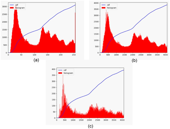
Figure 2. LDR2EDR process for dynamic range expansion. (a) original input histogram and its cumulative distribution; (b) histogram of the upsampled image and its cumulative distribution; (c) histogram of the downsampled image and its cumulative distribution.

3.2. EDR2HDR by Cumulative Histogram Learning

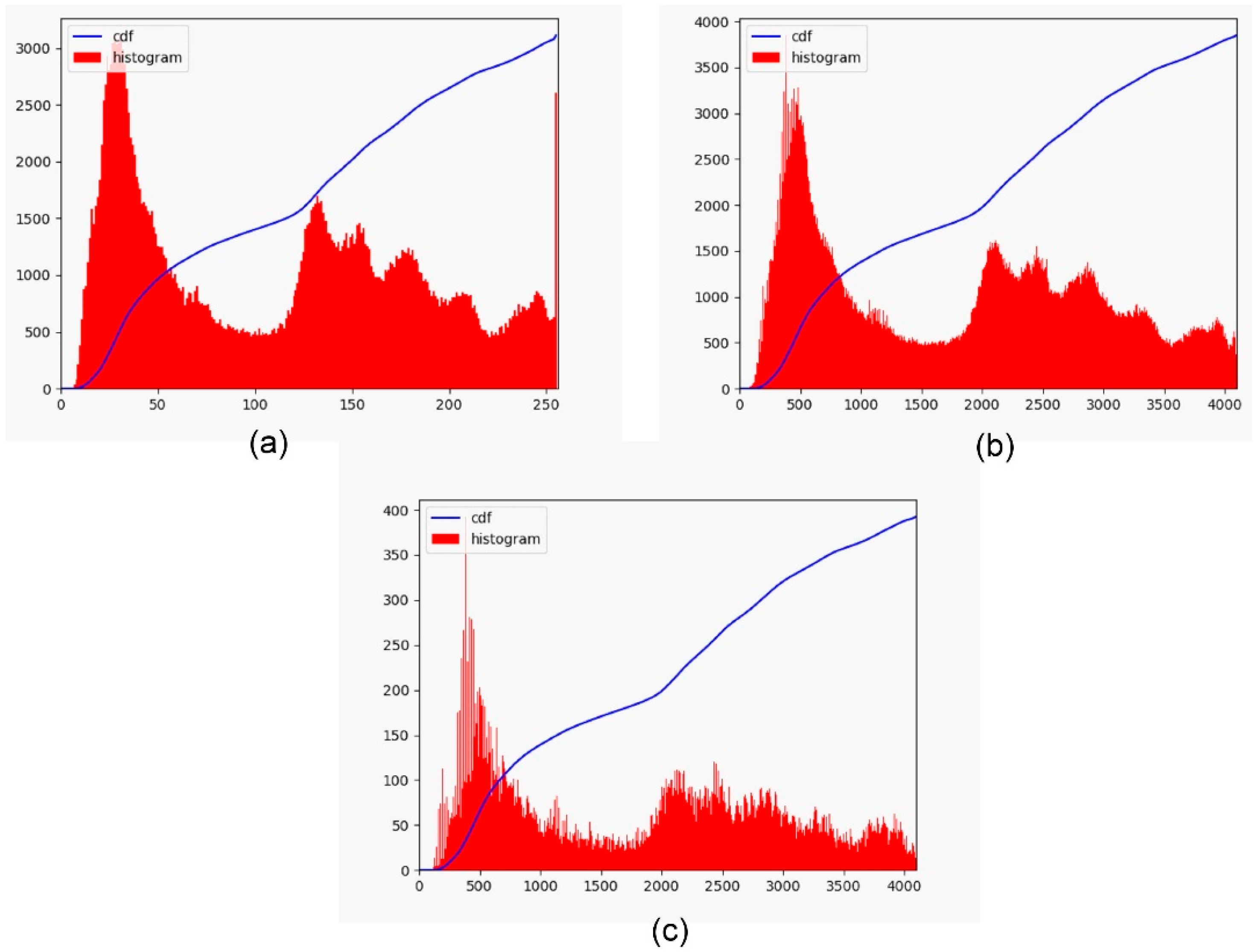
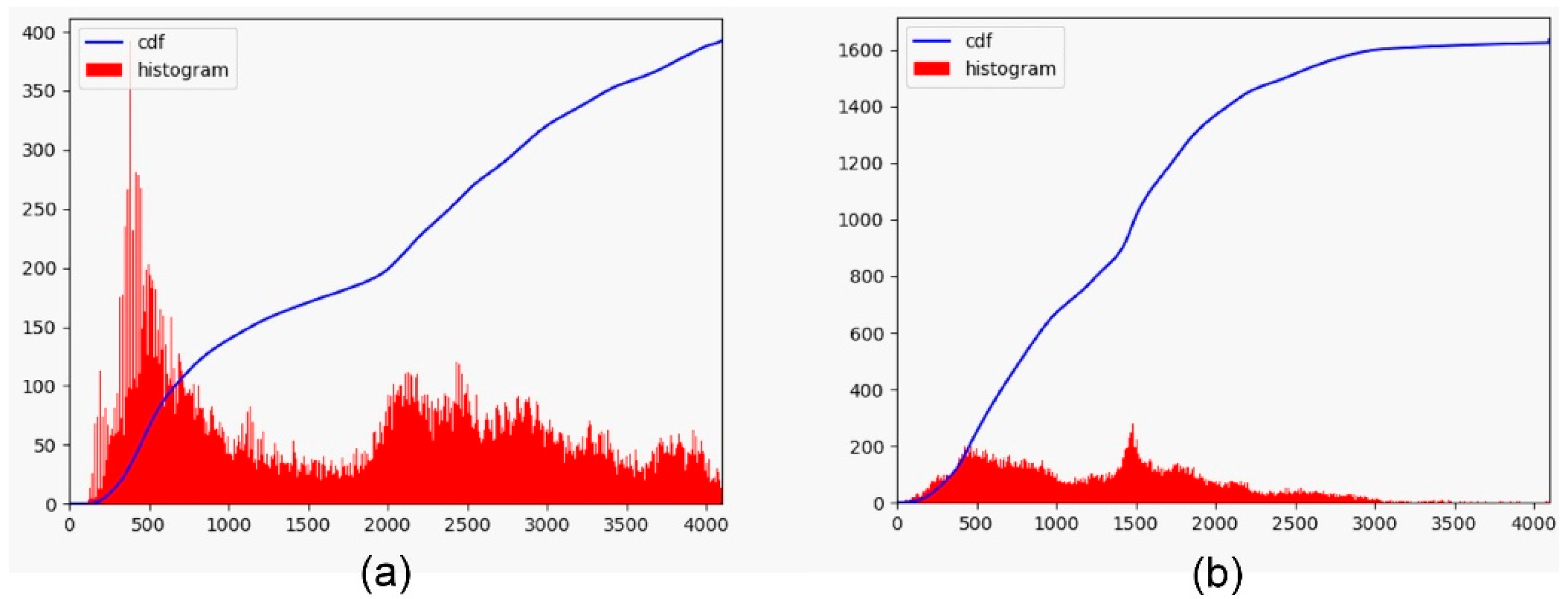
To produce a 12-bit HDR image from a 12-bit EDR image (EDR2HDR), we introduce a cumulative histogram learning technique based on deep neural networks. The basic idea is to learn pixel intensity distribution changes from EDR-HDR image pairs. To learn the intensity distribution of HDR images, we first convert 16-bit ground-truth HDR images into their 12-bit representations using proportional normalization as ground truths for histogram learning. Figure 3 demonstrates the histograms and CDFs of 12-bit EDR and HDR images, respectively. From the histogram of the EDR image, dark areas accumulate a large number of pixels, resulting in low contrast in the areas. The histogram of the HDR image is relatively flat and spreads out a wider range of pixel intensities to provide better contrast and details. Therefore, if we can change the pixel distribution of an EDR image such that its histogram is similar to the histogram of an HDR image, we can generate an HDR image with good contrast and details.

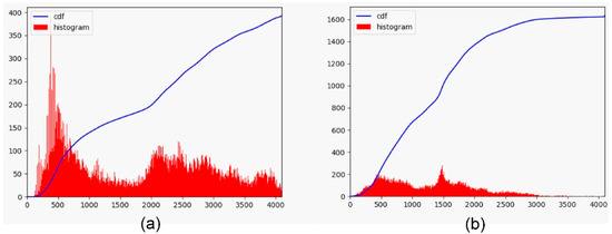
Figure 3. Histogram and its CDF of 12-bit EDR and HDR images. (a) histogram and its cumulative distribution of 12-bit EDR image; (b) histogram and its cumulative distribution of 12-bit HDR image.

Depending on the scene environment and camera settings, distributions of image histograms can be different. Therefore, it cannot formulate closed-form conversions between 12-bit EDR and HDR images. In the proposed approach, we introduce a technique for learning histogram transformations using deep neural networks. Due to the diversity of image histograms, learning directly from the intensity distributions cannot provide stable data for network training. However, the cumulative distribution histogram (or cumulative histogram) has simplicity and monotonically increasing properties. It is also within a fixed range, which facilitates data normalization and is suitable for model training. Nevertheless, the image intensity distribution can be reconstructed from the predicted cumulative histogram.

The proposed cumulative histogram learning architecture uses a fully connected neural network with four hidden layers. Both the input and output layers have 4096 neurons covering 2¹² different intensity values. Each hidden layer contains 8192 neurons and uses a rectified linear unit (ReLU) as the activation function. We added dropouts to the last two hidden layers and the dropout rate is set to 0.5. Although the model is relatively simple, it can effectively avoid overfitting and improve generalization ability. An issue related to the network output is the necessity of monotonically increasing, which guarantees non-negative values appearing in the image histogram. To ensure that this characteristic is maintained, the output cumulative curves are smoothed by a Savitzky–Golay filter [18] and then adjusted to produce monotonic constraints. Figure 4 shows the cumulative histogram results using curve smoothing and monotonic constraint. Figure 4a is the original output CDF and the corresponding histogram. The accumulation curve smoothed by the Savitzky–Golay filter and its image histogram are shown in Figure 4b. Although the slight jitter in the original curve prediction is alleviated, the histogram still contains negative values. To incorporate the monotonically increasing constraint, we force the first-order derivative of the curve to be nonnegative at any point. For two consecutive bins, if the cumulative value on the right is smaller, it is replaced by the cumulative value on the left. The processed curve is then used as the cumulative histogram and converted back to an image histogram. Figure 4c shows the final cumulative distribution and image histogram for this cumulative learning stage.

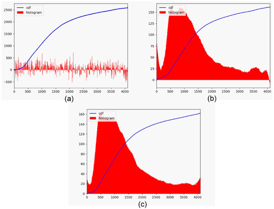
Figure 4. The cumulative histogram results. (a) Original output CDF and the corresponding histogram; (b) CDF and the corresponding histogram after curve smoothing; (c) CDF and the corresponding histogram after curve smoothing and monotonic constraint.

The proposed network is trained by minimizing the mean square error (MSE) between the input and target cumulative histograms. We set the batch size to 16, train for 300 epochs, and store the optimal weights during training. The adaptive moment estimation (ADAM) optimizer [19] is used with an initial learning rate of 0.001. The input images are resized to 512 × 512 for training and the cumulative histogram data are divided by 262,144 to normalize into the [0, 1] range. This also improves the convergence speed of the model. We do not use any common data enhancement methods, such as image rotation or horizontal flipping because the histogram distribution does not change. However, the data can be augmented by adjusting the image using various image formation pipelines.

After using the deep neural network, the predicted 12-bit HDR histogram can be obtained. Then, we use the 12-bit EDR image and the predicted 12-bit HDR histogram to perform histogram matching to derive the 12-bit HDR image. Figure 5 shows the histogram matching results. Figure 5a shows an LDR image, Figure 5b illustrates the resulting 12-bit HDR image (tone mapped) after histogram matching, and Figure 5c is the corresponding 16-bit HDR image (tone mapped) of Figure 5a as the ground-truth image. Compared with the original LDR image, the contrast adjusted according to the target histogram generated by cumulative distribution learning provides consistent details in dark and bright areas.

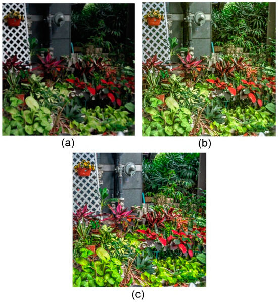
Figure 5. The histogram matching results. (a) LDR image; (b) resulting HDR image; (c) ground-truth image.

3.3. Fine-Tuning with Reinforcement Learning

After histogram matching, the 12-bit EDR and HDR images have similar pixel intensity distributions. However, due to the limited capabilities of the histogram for image representation, some details may still be lacking. To improve the consistency of regional pixel intensities, reinforcement learning is used to fine-tune the image in the spatial domain. The resulting 12-bit HDR image is first converted to its 16-bit HDR representation by multiplying all pixel intensities by 2⁴ for subsequent fine-tuning. The multi-agent reinforcement learning architecture, PixelRL, is used for image adjustment [20]. PixelRL modifies the asynchronous advantage actor critic (A3C) architecture into a fully convolutional form. It takes each pixel as an agent to gradually modify the image intensity through a pre-defined set of actions and find the optimal strategy that minimizes the squared error between the resulting image and the ground truth.

We use Chainer [21] and ChainerRL [22] to construct network architectures for deep reinforcement learning. The 16-bit HDR representation converted from the 12-bit HDR image is used as the input image I (s⁽⁰⁾), where s is the state of the agent and the corresponding16-bit HDR image of the original LDR image is the ground truth I^target. During training and testing, the agent selects appropriate actions for intensity adjustments from the set of actions listed in Table 1. In Table 1, we define a set of actions for image denoising and restoration that the agent can execute. These actions are empirically decided and are classical image-filtering algorithms. Our approach can select the adequate action in the action set to adjust the pixel value. After adjustment, the resulting image can be obtained. We include several classic image filters and values up/down in the action set. The reward is given by

$$r_i^t={\left(I_i^{target}-s_i^{\left(t\right)}\right)}^2-{\left(I_i^{target}-s_i^{(t+1)}\right)}^2,$$

(3)

where $I_i^{target}$ is the i-th pixel intensity of the ground truth. It calculates the squared error between the ground truth and the current image being decreased by action $a_i^{\left(t\right)}$. Therefore, maximizing the total reward is equivalent to minimizing the squared error between the final image $s^{t_{max}}$ and the ground truth I^target.

Table 1. The action set used by the agents for training and testing.

	Action	Filter Size	Parameter
1	box filter	5 × 5	-
2	bilateral filter	5 × 5	${\sigma }_c=1.0,{\sigma }_S=5.0$
3	bilateral filter	5 × 5	${\sigma }_c=0.1,{\sigma }_S=5.0$
4	median filter	5 × 5
5	Gaussian filter	5 × 5	$\mathsf{\sigma }=1.5$
6	Gaussian filter	5 × 5	$\mathsf{\sigma }=0.5$
7	pixel intensity + = 1	-
8	pixel intensity − = 1	-
9	pixel intensity + = 10	-
10	pixel intensity − = 10	-
11	pixel intensity + = 100	-
12	pixel intensity − = 100	-
13	do nothing	-

For training hyper-parameters, we use a batch size of 32 and perform data augmentation with 70 × 70 random cropping, horizontal image flipping, and random rotation. The ADAM optimizer and the polynomial learning rate strategy are used in the training process. The initial learning rate is set to 10⁻³ and is decreased by (episode/max_episode)^0.9 in each episode. We set the maximum episode max_episode to 3000, the length of each episode t_max to 15, and store weights every 20 episodes to select the best results.

4. Results

In the experiments, the proposed approach was implemented on a PC with a 64-bit Windows operating system and an Intel Core i7-9700 @ 3.00 GHz CPU with 16 G memory (Intel Corporation, Santa Clara, CA, USA). The used graphics card was an NVIDIA GeForce RTX 2070 SUPER (NVIDIA Corporation, Santa Clara, CA, USA). Our approach was also run on a computer with a 64-bit Ubuntu 18.04.6 LTS operating system and an AMD Ryzen 7 5800X CPU with 16 G memory (AMD, Santa Clara, CA, USA). We used an NVIDIA GeForce RTX 3090 graphics card (NVIDIA Corporation, Santa Clara, CA, USA). The proposed algorithm was mainly written in Python (version 3.10.0.) programming language.

We used the HDR-Real dataset as the training data [11] and the HDR-EYE dataset as the testing data [23]. The image resolution was 512 × 512. There were 9786 training image pairs and 46 testing image pairs in the original dataset. We established a subset by removing extreme images with a large proportion of overexposed and underexposed areas to improve learning performance. More specifically, if the number of pixels with intensity values greater than 249 or less than 6 exceeded 25% of the total pixels, the image was removed from the subset. After selection, there were 5673 image pairs in the HDR-Real training subset. For stage 1, we used the entire set of the HDR-Real dataset to extract histogram information for histogram learning because we only expanded an input 8-bit LDR image to a 12-bit HDR image. For stage 2, we converted a 12-bit HDR image to a 16-bit HDR image. We used a subset of the HDR-Real dataset for training to improve the performance of reinforcement learning.

First, the experiments were conducted in two stages. In the first stage, image histograms were extracted from the complete dataset for training. After predicting the histogram of the HDR image, we performed histogram matching on the EDR image to obtain a 12-bit HDR image. In the second stage, the pixel values of the resulting 12-bit HDR image were multiplied by 2⁴ and then adjusted pixel-by-pixel using a reinforcement learning framework to obtain a 16-bit HDR image. Figure 6 shows the resulting images of the proposed approach. In Figure 6, the left column shows LDR images, the second column shows the resulting 12-bit HDR images of stage 1, the third column shows the resulting 16-bit HDR images of stage 2, and the right column illustrates the ground-truth HDR images. Note that the second, third, and right columns of Figure 6 were tone-mapped representations. From the results, the proposed approach can reconstruct the desirable HDR images with high quality.

Figure 6. The resulting images of the proposed approach. The left column shows LDR images, the second column shows the resulting 12-bit HDR images of stage 1, the third column shows the resulting 16-bit HDR images of stage 2, and the right column illustrates the ground-truth HDR images. From the results, the proposed approach can reconstruct the desirable HDR images with high quality.

For the resulting HDR images, we used the mean-opinion-score of quality (Q_MOS) score from HDR-VDP-2 [24] for evaluation. The range of Q_MOS was 0 to 100. The higher the value, the better the image quality. Using 16-bit ground-truth HDR images as the reference images, the Q_MOS scores on the two stages of test datasets were 61.29 ± 2.71 and 61.54 ± 2.55, respectively. This represented a 0.25 improvement in the Q_MOS score given by the adjustment in the second stage. In addition, we adopted the peak signal-to-noise ratio (PSNR) and the structural similarity index (SSIM) [25] as performance metrics for quantitative comparison. Table 2 shows the evaluation results of the original images and the resulting images of the two stages. Both PSNR and SSIM evaluation metrics were significantly improved in the first stage. The results showed that the proposed approach can effectively learn the intensity distribution of the HDR and redistribute image intensity appropriately. In stage 2, through pixel-by-pixel adjustments based on reinforcement learning, PSNR and SSIM were further improved by 0.273 and 0.013, respectively.

Table 2. PSNR and SSIM evaluation results of original images and the resulting images of the two stages on tone-mapped images.

	Input Image	Stage 1	Stage 2
PSNR	14.218	19.314	19.587
SSIM	0.560	0.711	0.724

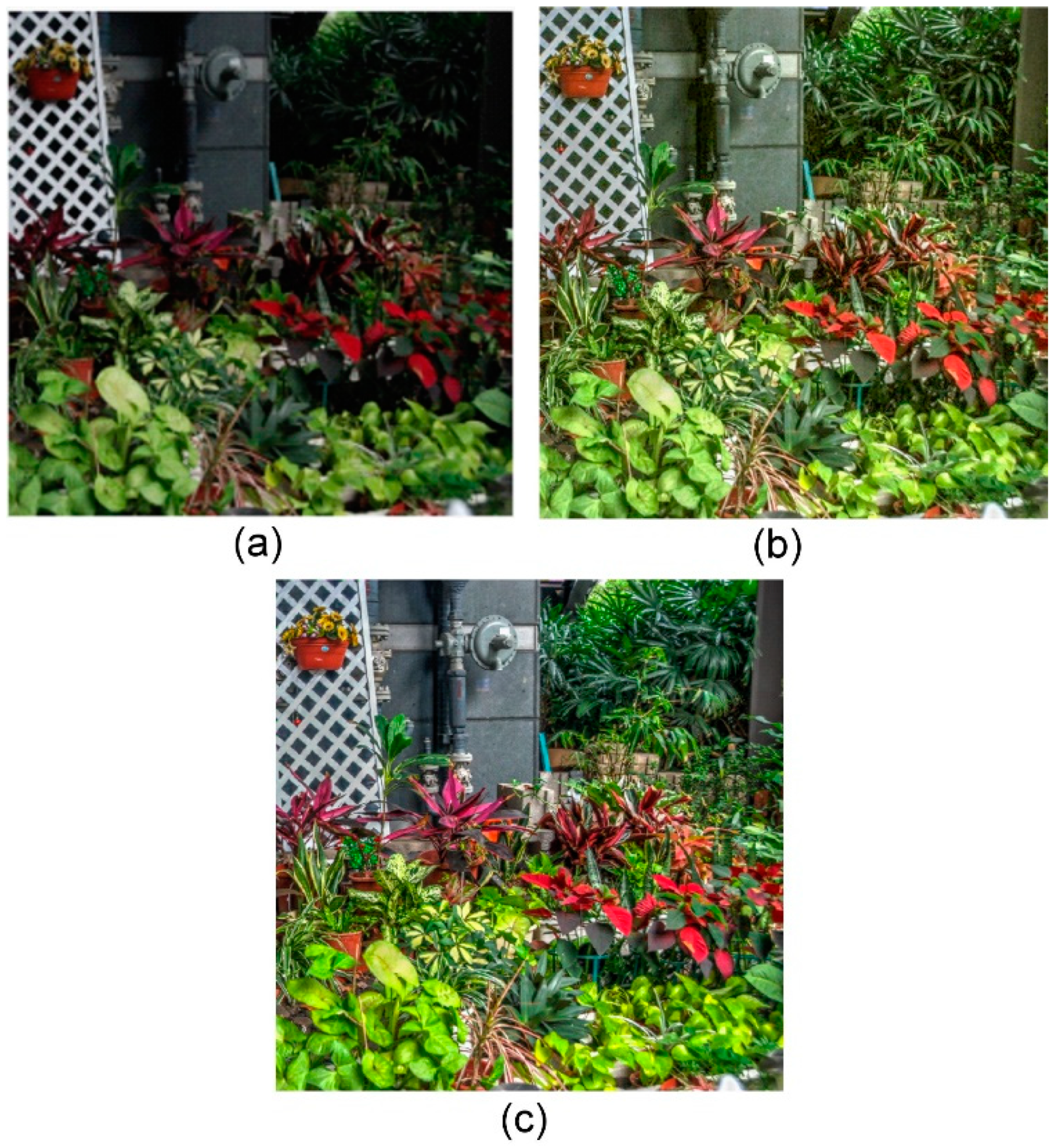
We selected four images from the HDR-EYE dataset for illustration. Figure 7 shows the input LDR images in the left column, our output HDR results in the middle column, and ground-truth HDR images in the right column. Images were converted to grayscale representations to better demonstrate contrast enhancement. As shown in the left column of Figure 7, the original images were partially underexposed, resulting in the loss of detailed textures. For example, the tree trunks in the first image, the stairs in the second image, building shadows in the third image, and the shadows under the parasols in the fourth image. All these difficult-to-identify details were greatly improved by the proposed technique, as shown in the middle column images of Figure 7. By redistributing pixel intensities based on predicted HDR histograms, pixels that were originally accumulated in dark areas due to underexposure can be more reasonably allocated. In the first result, the textures of the tree trunks became clearly visible and the changes in light and shadow on the building became more vivid. The second and third results were also improved for underexposure of stairs and building shadows. In the final result, the textural details of the building were clearly visible in the shadows and the seating areas under the parasols were no longer dark.

Figure 7. The resulting images are compared with the input LDR images and ground truth HDR images in tone-mapped grayscale representations. The left column shows LDR images, the middle column shows our output HDR images, and the right column illustrates the ground-truth HDR images.

In the last experiment, we compared the proposed approach with previous CNN-based methods, including HDRCNN [10], DrTMO [8], ExpandNet [14], and SingleHDR [11]. For existing works, pre-trained weights provided by the authors were used. The evaluation was performed on the HDR-EYE dataset to create HDR images. Table 3 shows the PSNR and SSIM scores on the tone-mapped images. We used 46 images for evaluation. The table shows that our approach can provide comparable results to the previous methods. In the PSNR metric, our results were better than HDRCNN and DrTMO. The proposed technique also performed better than HDRCNN in SSIM.

Table 3. Comparison of the proposed approach with the previous methods.

	PSNR	SSIM
HDRCNN [10]	17.782	0.683
DrTMO [8]	18.515	0.731
ExpandNet [14]	20.387	0.729
SingleHDR [11]	21.895	0.774
The Proposed Approach	19.587	0.724

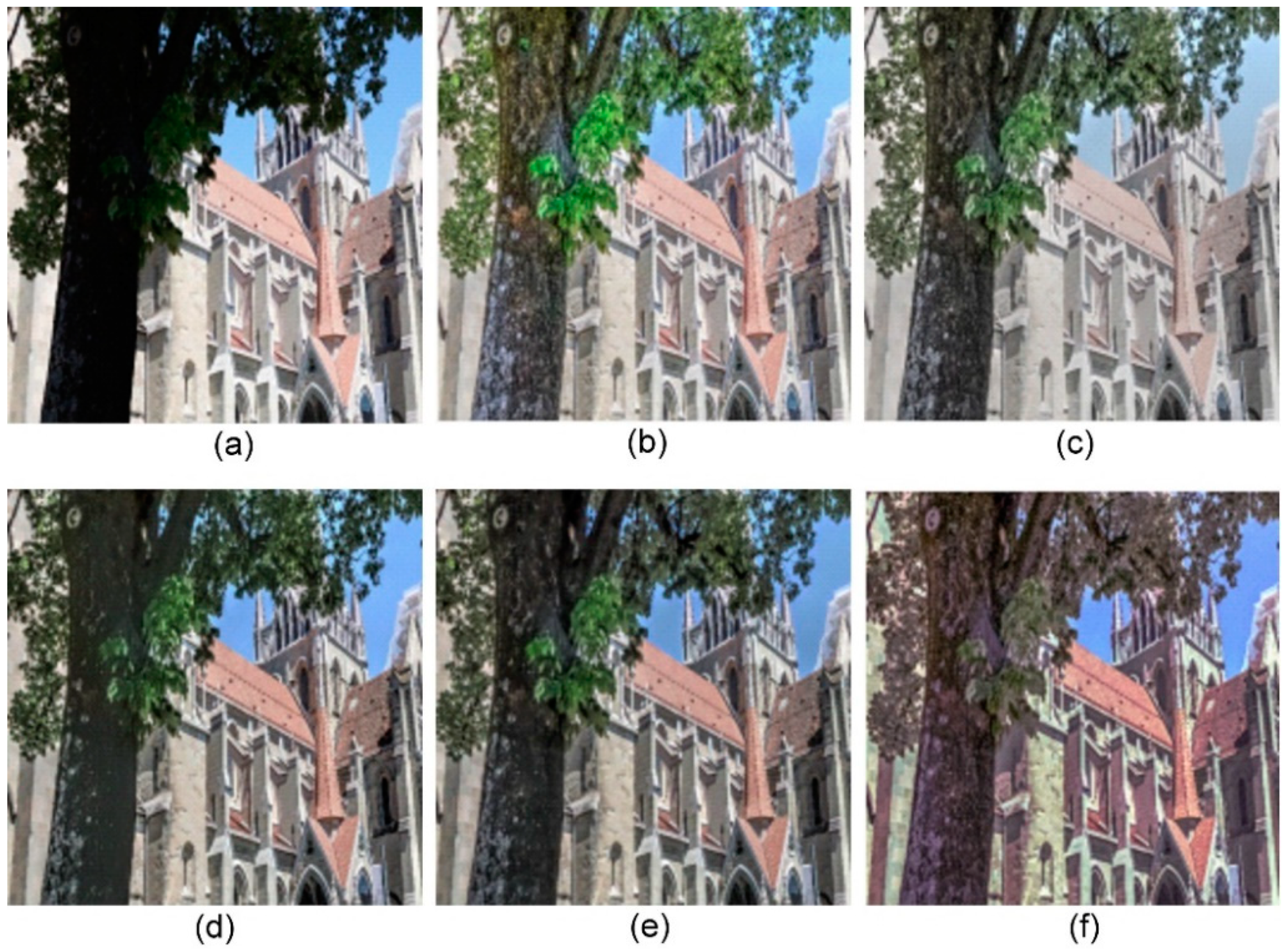
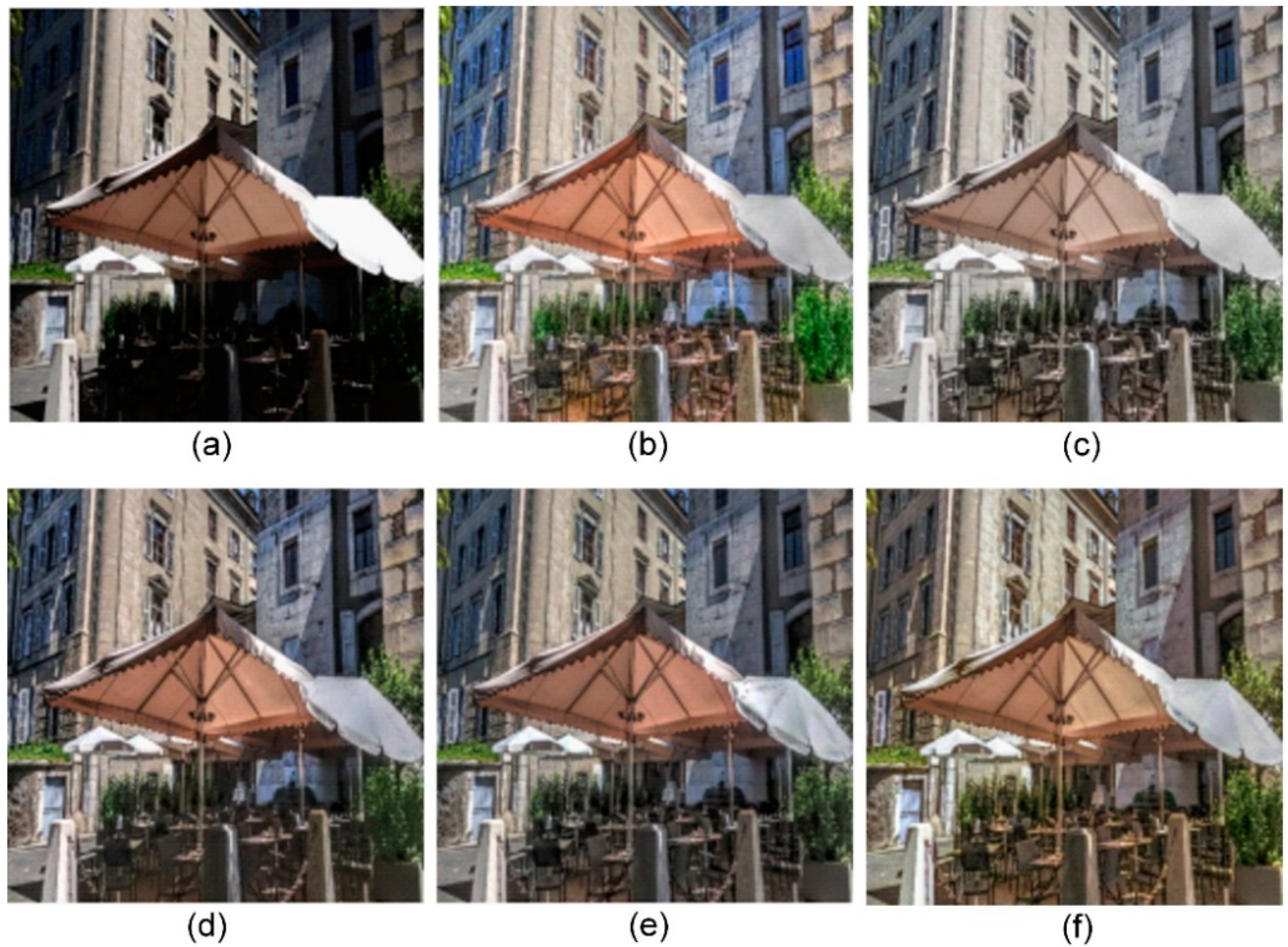
Figure 8, Figure 9, Figure 10 and Figure 11 show the tone-mapped results of single-image HDR reconstruction obtained through the previous methods and the proposed approach. Some underexposed areas were successfully reconstructed in all images, but some minor differences existed in hue and lightness. HDRCNN tended to variegate the image, but can also over-enhanced dark areas, resulting in a loss of contrast. The output from DrTMO, on the other hand, had blurred and washed-out tones and failed to faithfully represent the true colors of the scene. ExpandNet and SingleHDR cannot recover locally underexposed areas well. As shown in the results, the images obtained using the proposed approach restored details in dark areas, preserved contrast, and provided vivid color information.

Figure 8. The visual comparison of the proposed approach with the previous methods. (a) Input image, (b) HDRCNN, (c) DrTMO, (d) ExpandNet, (e) SingleHDR, and (f) the proposed approach.

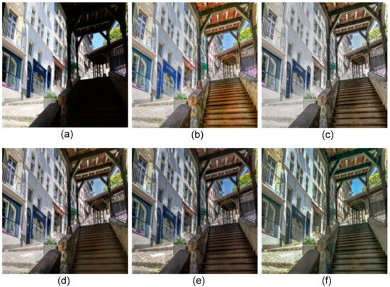
Figure 9. The visual comparison of the proposed approach with the previous methods. (a) Input image, (b) HDRCNN, (c) DrTMO, (d) ExpandNet, (e) SingleHDR, and (f) the proposed approach.

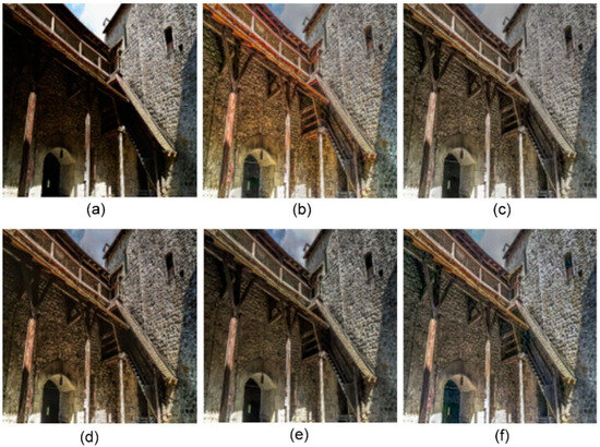
Figure 10. The visual comparison of the proposed approach with the previous methods. (a) Input image, (b) HDRCNN, (c) DrTMO, (d) ExpandNet, (e) SingleHDR, and (f) the proposed approach.

Figure 11. The visual comparison of the proposed approach with the previous methods. (a) Input image, (b) HDRCNN, (c) DrTMO, (d) ExpandNet, (e) SingleHDR, and (f) the proposed approach.

For qualitative comparison, Figure 8, Figure 9, Figure 10, and Figure 11 were evaluated qualitatively by 36 subjects. The subjects assessed the resulting images generated by the previous methods and our approach by assigning a score from 1 (poor) to 5 (good). Table 4 shows the average scores of the resulting images for the approaches. The average scores of HDRCNN [10], DrTMO [8], ExpandNet [14], SingleHDR [11], and the proposed approach were 3.25, 3.26, 3.74, 3.86, and 3.63, respectively. Our approach was better than HDRCNN and DrTMO, but slightly worse than ExpandNet and SingleHDR. Hence, the proposed approach can maintain a certain quality for reconstructing comparable HDR images.

Table 4. Qualitative evaluation.

	Average Score
HDRCNN [10]	3.25
DrTMO [8]	3.26
ExpandNet [14]	3.74
SingleHDR [11]	3.86
The Proposed Approach	3.63

5. Conclusions

We have proposed a two-stage approach for reconstructing an HDR image from a single LDR image-based histogram learning. We introduce a cumulative histogram learning technique based on deep neural networks for dynamic range expansion. The proposed approach predicts HDR intensity distributions from LDR histograms and reallocates image pixels through histogram matching. HDR images are then reconstructed using reinforcement learning and pixel-level rewards for local consistency adjustments. The experiments are conducted on HDR-Real and HDR-EYE datasets. The quantitative evaluations on HDR-VDP-2, PSNR, and SSIM demonstrate the effectiveness of the proposed approach compared to the previous methods. In addition, the qualitative evaluations show that the proposed approach can maintain a certain quality for reconstructing comparable HDR images. Hence, we can obtain favorable HDR images.

In the proposed approach, we use a network architecture with only fully connected layers for histogram learning. This architecture needs a large number of parameters and takes a lot of memory. We will develop a more suitable network architecture for experiments and test the proposed approach on different datasets [24]. Moreover, the proposed approach processes the three color channels separately in the RGB color space and then merges them into one color image. However, it may cause chromatic aberration in the resulting images. We will perform joint learning on all channels of images for improvement.

References

- Debevec, P.E.; Malik, J. Recovering high dynamic range radiance maps from photographs. In Proceedings of the SIGGRAPH 1997: 24th Annual Conference on Computer Graphics and Interactive Techniques, Los Angeles, CA, USA, 3–8 August 1997; pp. 369–378. [Google Scholar]
- Kalantari, N.K.; Ramamoorthi, R. Deep high dynamic range imaging of dynamic scenes. ACM Trans. Graph. (TOG) 2017, 36, 144. [Google Scholar] [CrossRef]
- Qiao, Z.; Yi, H.; Wen, D.; Han, Y. Robust HDR reconstruction using 3D patch based on two-scale decomposition. Signal Process. 2024, 219, 109384. [Google Scholar] [CrossRef]
- Yan, Q.; Gong, D.; Shi, Q.; Hengel, A.v.d.; Shen, C.; Reid, I.; Zhang, Y. Attention guided network for ghost-free high dynamic range imaging. In Proceedings of the IEEE/CVF Conference on Computer Vision and Pattern Recognition (CVPR 2019), Long Beach, CA, USA, 15–20 June 2019; pp. 1751–1760. [Google Scholar]
- Lin, H.Y.; Kao, C.C. Hierarchical bit-plane slicing for high dynamic range image stereo matching. IEEE Trans. Instrum. Meas. 2021, 70, 1–11. [Google Scholar] [CrossRef]
- Lin, Y.R.; Lin, H.Y.; Lin, W.C. Single image HDR synthesis with histogram learning. In Proceedings of the 26th Iberoamerican Congress on Pattern Recognition (CIARP 2023), Coimbra, Portugal, 27–30 November 2023; pp. 108–122. [Google Scholar]
- Rempel, A.G.; Trentacoste, M.; Seetzen, H.; Young, H.D.; Heidrich, W.; Whitehead, L.; Ward, G. LDR2HDR: On-the-fly reverse tone mapping of legacy video and photographs. ACM Trans. Graph. (TOG) 2007, 26, 39. [Google Scholar] [CrossRef]
- Endo, Y.; Kanamori, Y.; Mitani, J. Deep reverse tone mapping. ACM Trans. Graph. (TOG) 2017, 36, 177. [Google Scholar] [CrossRef]
- Lee, S.; An, G.H.; Kang, S.J. Deep recursive HDRI: Inverse tone mapping using generative adversarial networks. In Proceedings of the European Conference on Computer Vision (ECCV 2018), Munich, Germany, 8–14 September 2018; pp. 596–611. [Google Scholar]
- Eilertsen, G.; Kronander, J.; Denes, G.; Mantiuk, R.K.; Unger, J. HDR image reconstruction from a single exposure using deep CNNs. ACM Trans. Graph. (TOG) 2017, 36, 178. [Google Scholar] [CrossRef]
- Liu, Y.L.; Lai, W.S.; Chen, Y.S.; Kao, Y.L.; Yang, M.H.; Chuang, Y.Y.; Huang, J.B. Single-image HDR reconstruction by learning to reverse the camera pipeline. In Proceedings of the IEEE/CVF Conference on Computer Vision and Pattern Recognition (CVPR 2020), Seattle, WA, USA, 14–19 June 2020; pp. 1651–1660. [Google Scholar]
- Santos, M.S.; Ren, T.I.; Kalantari, N.K. Single image HDR reconstruction using a CNN with masked features and perceptual loss. arXiv 2020, arXiv:2005.07335. [Google Scholar] [CrossRef]
- Wu, G.; Song, R.; Zhang, M.; Li, X.; Rosin, P.L. LiTMNet: A deep CNN for efficient HDR image reconstruction from a single LDR image. Pattern Recognit. 2022, 127, 108620. [Google Scholar] [CrossRef]
- Marnerides, D.; Bashford-Rogers, T.; Hatchett, J.; Debattista, K. Expandnet: A deep convolutional neural network for high dynamic range expansion from low dynamic range content. Comput. Graph. Forum 2018, 37, 37–49. [Google Scholar] [CrossRef]
- Guo, C.; Jiang, X. LHDR: HDR reconstruction for legacy content using a lightweight DNN. In Proceedings of the 16th Asian Conference on Computer Vision (ACCV 2022), Macau, China, 4–8 December 2022; pp. 3155–3171. [Google Scholar]
- Cao, G.; Zhou, F.; Liu, K.; Bozhi, L. A brightness-adaptive kernel prediction network for inverse tone mapping. Neurocomputing 2021, 464, 1–14. [Google Scholar] [CrossRef]
- Kim, S.Y.; Oh, J.; Kim, M. Deep SR-ITM: Joint learning of super-resolution and inverse tone-mapping for 4K UHD HDR applications. In Proceedings of the IEEE/CVF International Conference on Computer Vision (ICCV 2019), Seoul, Republic of Korea, 27 October–2 November 2019; pp. 3116–3125. [Google Scholar]
- Savitzky, A.; Golay, M.J. Smoothing and differentiation of data by simplified least squares procedures. Anal. Chem. 1964, 36, 1627–1639. [Google Scholar] [CrossRef]
- Kingma, D.P.; Ba, J. Adam: A method for stochastic optimization. arXiv 2014, arXiv:1412.6980. [Google Scholar]
- Furuta, R.; Inoue, N.; Yamasaki, T. PixelRL: Fully convolutional network with reinforcement learning for image processing. IEEE Trans. Multimed. 2019, 22, 1704–1719. [Google Scholar] [CrossRef]
- Tokui, S.; Okuta, R.; Akiba, T.; Niitani, Y.; Ogawa, T.; Saito, S.; Suzuki, S.; Uenishi, K.; Vogel, B.; Yamazaki, V.H. Chainer: A deep learning framework for accelerating the research cycle. In Proceedings of the 25th ACM SIGKDD International Conference on Knowledge Discovery & Data Mining, Anchorage, AK, USA, 4–8 August 2019; pp. 2002–2011. [Google Scholar]
- Fujita, Y.; Nagarajan, P.; Kataoka, T.; Ishikawa, T. ChainerRL: A deep reinforcement learning library. J. Mach. Learn. Res. 2021, 22, 1–14. [Google Scholar]
- Nemoto, H.; Korshunov, P.; Hanhart, P.; Ebrahimi, T. Visual attention in LDR and HDR images. In Proceedings of the 9th International Workshop on Video Processing and Quality Metrics for Consumer Electronics (VPQM 2015), Chandler, AZ, USA, 5–6 February 2015. [Google Scholar]
- Mantiuk, R.; Kim, K.J.; Rempel, A.G.; Heidrich, W. HDR-VDP-2: A calibrated visual metric for visibility and quality predictions in all luminance conditions. ACM Trans. Graph. (TOG) 2011, 30, 40. [Google Scholar] [CrossRef]
- Eilertsen, G.; Hajisharif, S.; Hanji, P.; Tsirikoglou, A.; Mantiuk, R.K.; Unger, J. How to cheat with metrics in single-image HDR reconstruction. In Proceedings of the 2021 IEEE/CVF International Conference on Computer Vision Workshops (ICCVW), Montreal, BC, Canada, 11–17 October 2021. [Google Scholar]
Disclaimer/Publisher’s Note: The statements, opinions and data contained in all publications are solely those of the individual author(s) and contributor(s) and not of MDPI and/or the editor(s). MDPI and/or the editor(s) disclaim responsibility for any injury to people or property resulting from any ideas, methods, instructions or products referred to in the content. |
© 2024 by the authors. Licensee MDPI, Basel, Switzerland. This article is an open access article distributed under the terms and conditions of the Creative Commons Attribution (CC BY) license (https://creativecommons.org/licenses/by/4.0/).