MDSA: A Dynamic and Greedy Approach to Solve the Minimum Dominating Set Problem

Abstract

The graph theory is one of the fundamental structures in computer science used to model various scientific and engineering problems. Many problems within the graph theory are categorized as NP-hard and NP-complete. One such problem is the minimum dominating set (MDS) problem, which seeks to identify the minimum possible subsets in a graph such that every other node in the subset is directly connected to a node in this subset. Due to its inherent complexity, developing an efficient polynomial-time method to address the MDS problem remains a significant challenge in graph theory. This paper introduces a novel algorithm that utilizes a centrality measure known as the Malatya Centrality to effectively address the MDS problem. The proposed algorithm, called the Malatya Dominating Set Algorithm (MDSA), leverages centrality values to identify dominating sets within a graph. It extends the Malatya centrality by incorporating a second-level centrality measure, which enhances the identification of dominating nodes. Through a systematic and algorithmic approach, these centrality values are employed to pinpoint the elements of the dominating set. The MDSA uniquely integrates greedy and dynamic programming strategies. At each step, the algorithm selects the most optimal (or near-optimal) node based on the centrality values (greedy approach) while updating the neighboring nodes’ criteria to influence subsequent decisions (dynamic programming). The proposed algorithm demonstrates efficient performance, particularly in large-scale graphs, with time and space requirements scaling proportionally with the size of the graph and its average degree. Experimental results indicate that our algorithm outperforms existing methods, especially in terms of time complexity when applied to large datasets, showcasing its effectiveness in addressing the MDS problem.

1. Introduction

Many complex problems in engineering and scientific disciplines may require mathematical modeling due to optimization and efficiency issues. The problems under graph theory are widely used solutions in mathematical modeling. One of these approaches is the minimum dominating set (MDS) problem, which is also NP-hard. The MDS problem aims to determine the minimum possible set of nodes in a graph; of course, each node in these sets must be connected to the other nodes in the set by a dominance node. Fomin et al. classified the MDS problem as NP-hard and showed the exponential increase in computational complexity for methods that produce exact solutions [1]. NP-hard problems are as hard or harder to solve than problems defined in NP, which are solved in polynomial time. If a problem is defined in the NP-hard class, it is not necessarily a decision problem, it may not have a question with a “yes/no” answer, and its solution may not be simple to verify. These problems generally have exponential time complexity. If a problem in the NP-hard class can be solved in polynomial time, then it is classified as NP-complete.

The algorithms developed to solve the MDS problem provide highly effective solutions to the main problems such as optimizing resource allocation and reducing costs in complex network structures where a complex network is a network with non-trivial topological features that do not occur in lattice or simple graphs; on the contrary, they occur in social networks [2,3,4], wireless networks [5], sensor networks [6], transportation [7], biology [8], etc. The work performed in [9] to improve routing efficiency in wireless networks can give an idea about the real-life application of the MDS problem. In addition, the methodologies proposed to solve MDS can be effective in various contexts including Hopfield networks, maximum clique identification, and maximum independent set isolation [10]. The application domain of MDS is quite wide and there is a scarcity of efficient algorithms to solve the MDS problem for these application domains [11,12,13,14].

Since the MDS problem is NP-hard and it is generally not practical to find an exact solution in large-scale graphs, methods aiming to obtain results close to the optimal solution have been proposed in the literature. These methods are classified as approximation algorithms, heuristic and metaheuristic algorithms that provide fast solutions, parameterized algorithms with features arranged according to the characteristics of the problem, and integer linear programming that can be applied to certain situations [15,16,17,18,19]. The application of greedy approaches in these methods can offer significant advantages in the context of simplicity, speed, and reduced computational load. This makes them useful in quickly obtaining appropriate solutions when faced with very large or complex examples [5].

The method applied to the MDS problem is expected to be fast and therefore have low algorithm complexity, especially when considering large graphs. The studies proposed in the literature focus on time complexity and obtain better measurements than the traditional exhaustive $\mathrm{\Omega }\left(2^n\right)$ method for graphs with n nodes. An algorithm that reduces the time complexity to $O\left({1.81}^n\right)$ is presented in [20]. A greedy search algorithm finds the optimal or nearly optimal solution with $O\left(n^3\right)$ time complexity [2]. In another study, the time complexity of the algorithm is reported as $O\left(n^{2}lgn\right)$ [21]. A special spanning tree, the Kmax tree, is introduced using basic cut sets with $O(n^2+\mathrm{m})$ complexity and then a series of steps are executed [22].

This study aims to contribute to the literature by proposing a new approach using the Malatya centrality values for the MDS problem with complexity $\Theta \left(n\times d\right)$. The Malatya centrality algorithm was first presented in [23] and it is updated and improved by our work. The Malatya centrality algorithm is used to compute centrality values of each node in the first and second phases. The proposed algorithm extends the idea of Malatya centrality and makes it consistent with the given domain in the minimum dominating set problem. Based on our experimental findings, this perspective effectively saves time and resources by providing optimum or near-optimum answers that facilitate finding a fast and feasible solution for the MDS problem. The main contributions of the proposed method are as follows:

• Inspired by the Malatya centrality algorithm, this concept was applied to the MDS problem and is the first study in the literature using it.
• A greedy search strategy application that applies the same steps in each run, produces the same result, and provides robust, efficient, and effective solutions.
• Optimization in terms of time and resource complexity thanks to a dynamic search strategy that updates the graph at each step.
• It is easily applicable to large graphs since it is designed to have polynomial time and resource complexities.
• Increasing its preference rate in application areas since it produces optimum or nearly optimum solutions for the MDS problem.
• It is suitable for a wide range of application scenarios since it has the ability to find minimum dominant sets for all memory allocated graph structures.

In this study, comprehensive experimental evaluations were conducted to assess the effectiveness and performance of the proposed algorithm. The algorithm was validated using DIMACS, BHOSLIB, SNAP, and network repository datasets. It consistently achieved optimal dominating set results with notably short execution times across these datasets. Comparative results with algorithms from the literature showed that the proposed algorithm excels particularly in terms of speed on large datasets. The consistent performance of our algorithm, especially on large graphs, underscores its practicality for real-world applications. These findings indicate that the proposed algorithm provides an effective and efficient solution for both small and large graphs.

This article is structured as follows: Section 2 reviews active studies in the literature addressing the dominating set problem. Section 3 discusses the definition of the dominating set problem and its NP-hard nature. Section 4 provides a detailed explanation of the proposed Malatya Dominating Set Algorithm. Section 5 presents the implementation results of the algorithm and its comparison with competitive methods. Finally, Section 6 concludes the article.

2. Related Works

Finding the dominant sets in a graph is closely related to understanding the nature of the data or structure to which it is applied. The complexity of the problem and the exponential solution encourage the continuous discovery of innovative strategies that work faster. Greedy algorithms, in particular, have provided remarkable solutions to this NP-hard complexity. This section reviews recent developments in the field and presents the variety of approaches and the ongoing development of algorithms that address the MDS problem.

Chalupa and Blum proposed a method that identifies important nodes and edges in a given graph and thus reveals shortcuts in the graph [24]. Their proposed method has been tested on real-world datasets and its effectiveness has been demonstrated in network analysis. Following this paper, Chalupa proposed a new order-based random local search (RLS_o) algorithm to solve the MDS problem [17]. Experimental results show that the RLS_o algorithm outperforms both the greedy algorithm and two ACO-based (ant colony optimization) metaheuristic algorithms and is also scalable to large graphs. Wang et al. proposed FastMWDS, a fast local search method, to tackle the MDS problem [25], especially for large-scale graphs. This algorithm handles large-scale networks effectively by using heuristic techniques. When compared to other heuristic approaches, the study showed better performance both in solution quality and execution time. Fan et al. introduced an efficient local search algorithm to solve the MDS problem in large graphs [26]. This algorithm, named Score Checking and Best-picking with Probabilistic Walk (ScBppw), utilizes a probabilistic approach combined with a Tabu Search strategy to diversify the search process. Cai et al. introduced an efficient local search algorithm named FastDS to address the MDS problem [27]. This algorithm integrates two main ideas: a novel local search framework and a construction procedure with inference rules. Notably, FastDS has been reported to achieve significantly better solutions compared to state-of-the-art algorithms on large graphs. The time complexity of FastDS is $O(nlogn+m)$, where n represents the number of vertices and m represents the number of edges. Zhong et al. have designed a unified $O\left(ln\delta \right)$-approximation algorithm for the generalized MDS problem, with the concept of submodular and weakly submodular potential functions [28]. The authors have stated that this algorithm either provides the best result among the existing approximation algorithms for specific versions or presents the first approximate solution. In their research, Sun et al. proposed a local search algorithm for the minimum positive influence dominating set (MPIDS) problem that includes reduction-based initialization, a new node exchange strategy, and a general local search framework [29]. This method shows improvement over previous MPIDS solutions on various graph benchmarks, presenting a new way to tackle NP-hard combinatorial optimization problems in graph theory. Nakanishi introduced a method to pinpoint nodes that form the MDS in graphs with a minimum degree of three, transforming these graphs into 2-connected forms with specific cycle lengths [30]. This approach, which cleverly labels nodes within these cycles, offers a partial solution to the APX-complete MDS problem for cubic graphs, contributing to the field of graph theory with a novel perspective on combinatorial optimization challenges. In another study, Casado et al. tackle the NP-hard MDS problem by proposing an Iterated Greedy algorithm, showcasing its effectiveness in finding optimum or nearly optimum solutions through a comparative study with exact and up-to-date algorithms [31]. Their algorithm achieves an average deviation of only 0.04% from optimal solutions for solvable instances and 1.23% for more complex cases, thus presenting a significant advancement in solving combinatorial optimization problems in graph theory. Zhang et al. developed a new greedy algorithm to tackle the Minimum Edge Connected Dominating Set (MECDS) problem in wireless sensor networks, focusing on edge fault tolerance [32]. Their algorithm achieves an important improvement in approximation ratios and sets a new standard for constructing robust virtual backbones against link failures. Chen et al. introduce a local search algorithm, DeepOpt-MWDS, for solving the Minimum Weight Dominating Set (MWDS) problem [33]. By adjusting the number of nodes added or removed based on candidate solution feedback, employing reduction rules for initial solution construction, and integrating a novel configuration checking strategy to minimize local search cycling, the algorithm outperforms existing heuristics in both efficiency and effectiveness on a wide range of graph benchmarks. That study not only demonstrates the superior performance of DeepOpt-MWDS on diverse datasets but also showcases its adaptability to other NP-hard problems, marking a contribution to the field of combinatorial optimization. In their study, Argiroffo et al. explore the polyhedral aspects of locating, open locating and locating total dominating sets within graphs, offering a fresh perspective on these variations of the classical MDS problem. By developing linear relaxations and examining their combinatorial structures, the authors successfully apply polyhedral techniques to fully describe these sets for special graph types. Akbay et al. introduce Adapt-CMSA, a self-adaptive variant of the Construct, Merge, Solve and Adapt (CMSA) algorithm, aimed at addressing the parameter sensitivity observed in the original CMSA algorithm [34]. By automating parameter adjustments, Adapt-CMSA reduces the need for extensive parameter tuning across different problem instances, demonstrating its effectiveness on the minimum positive influence dominating set problem (MPIDS). In their research, Chakraborty et al. propose constant-factor approximation algorithms designed to solve the MDS problem within specific subclasses of string graphs (a string graph can be defined as a graph where edges are formed by the intersections of curves, and each curve is represented by a node), with a particular emphasis on unit Bk-VPG graphs and vertically stabbed L-graphs [35]. By developing algorithms with guaranteed approximation ratios for these complex graph types, the study addresses open questions and extends previous research findings. The idea of finding a solution to the dominating set problem using centrality measures was previously proposed by Rehm et al. [36]. In their study, the authors applied the Shapley value centrality measures derived from game theory with a two-stage algorithm and applied them to real-world problems.

Solving the MDS problem presents a perspective from the implementation of unified approximation algorithms and the introduction of novel local search strategies to the exploration of polyhedral techniques and self-adaptive algorithms; the scope of research is broad and dynamic. Each study contributes unique insights into tackling the MDS problem, whether through refining algorithmic accuracy, enhancing computational efficiency, or expanding the theoretical understanding of underlying graph structures. Notably, these efforts not only advance the state of the art in solving the MDS problem but also illustrate the adaptability of these algorithms to a spectrum of related problems and graph subclasses. The highlighted works underscore the enduring relevance of the MDS problem and the innovative approaches being developed to tackle it. Greedy algorithms, in particular, stand out for their significant contributions, demonstrating the rich potential for further research in this area. As the field progresses, it is anticipated that these foundational efforts will pave the way for even more sophisticated solutions, enhancing our ability to solve the MDS problem and its variants across increasingly complex graph structures.

3. The Dominating Set Problem

Definition 1 provides the characterization of a dominating set.

Definition 1.

Consider  $G=(V,E)$  to represent a graph, and if  $D\subseteq V, \forall v\in V v\in D$  or  $v\in V\backslash D$  and  $v\in N\left(D\right)$, N is the set of neighbours of nodes in D, then,  $D$  is called a dominating set. A dominating set encompasses all adjacent nodes within its neighborhood.

Definition 2.

Consider G, D, N, and V as in Definition 1; when  $D$  possesses the smallest possible number of elements, it is referred to as the MDS.

The minimum dominating set problem is to determine dominating set of minimum size, and try to find its cardinality. The dominating set problem falls into the NP-hard category, meaning that it is almost impossible to find the most suitable solution quickly with current computer technology. More detailed information can be found in the study [11] about the dominating set. It can be seen that solving the MDS problem with a polynomial-time algorithm is NP-hard with the proof by the following contradiction via the SAT problem [37]:

Assumption 1.

Assume that the MDS problem is not NP-hard and there is an algorithm, running in polynomial time, to solve this problem.

Contradiction 1.

If there is an algorithm to solve the MDS problem with polynomial time complexity, then this algorithm should solve the SAT problem with polynomial time complexity. However, it is well known that the SAT is an NP-hard problem, which leads to a contradiction.

Proof: 

The Boole Satisfiability Problem (SAT) is the problem of determining whether a given Boole formula is satisfiable, and it is NP-hard. This problem is expressed as $F=(C_1\wedge C_2\wedge \dots \wedge C_m)$, where each $C_j$ is a clause consisting of a set of literals (for example, ${\mathrm{C}}_1=({\mathrm{x}}_1\vee \overline{{\mathrm{x}}_2}\vee {\mathrm{x}}_3)$). To reduce the SAT problem to the MDS problem, we follow these steps:

• For each variable $x_i$, create a node $v_i$.
• For each clause $C_j$, create a node $c_j$.
• If a variable $x_i$ appears positively in a clause $C_j$, add an edge between $v_i$ and $c_j$. If the negation $\overline{{\mathrm{x}}_{\mathrm{i}}}$ appears in $C_j$, also add an edge between $v_i$ and $c_j$.

After this transformation, all nodes in the graph are connected such that the Boolean formula is satisfied. Specifically, each clause node $c_j$ must be adjacent to at least one variable node $v_i$. If the resulting graph has a dominating set, this set corresponds to a set of variables that satisfy the SAT problem. Thus, if the graph has a dominating set, the formula $F$ is satisfiable.

Since the SAT is an NP-hard problem, solving it in polynomial time is impossible. Therefore, the assumption that the MDS problem can be solved in polynomial time leads to a contradiction. The assumption that the MDS problem is not NP-hard is false. Hence, the MDS problem is NP-hard. □

4. Malatya Dominating Set Algorithm (MDSA)

A robust algorithm that is capable of finding the solution of the MDS for all graphs is proposed in this paper. It finds efficient solutions, mostly by saving a significant amount of time. The basis of our algorithm’s fastness is the Malatya centrality algorithm and the idea of minimizing the network by marking nodes in each iteration. Karci et al. proposed a new algorithm to reveal the strength of the nodes of the given graph relative to each other, and a centrality value of the nodes is calculated using the node degrees, they named this algorithm as Malatya centrality algorithm (MCA) [23]. Subsequently, they applied this algorithm to address the minimum node cover in any graph [38]. They applied the MCA to address the maximum independent set and called it as Malatya Maximum Independent Set Algorithm. At the same time, the same group of authors proposed an algorithm to solve the minimum node cover problem using the MCA [39].

In [40], we published a very brief and draft version of this paper. The method we propose in this paper includes the following improvements over the method proposed in the first publication:

• The previous version contains the initial Malatya centrality value equation as follows:

  $${\Psi }_1\left(v_i\right)=\left({\sum }_{v_i\in V,v_j\in V_N\left(v_i\right)}{\displaystyle \frac{d\left(v_i\right)}{d\left(v_j\right)}}\right)$$

  (1)

The difference between the first Malatya centrality value equations (Equations (1) and (2)) is significant, as the centrality values change relative to each other. These changes in centrality values affect the dominating set.

• In the previous version, the selected nodes and their neighbors are removed from the given graph. In the current version, only the selected node is removed from the graph; however, the neighbors of the selected node are not removed, except for those with active degrees equal to 2.
• The previous version finds an independent dominating set and does not aim to find the optimal solution. In contrast, the current version finds the dominating set/minimum dominating set.
• Extensive experiments and competitive method comparisons were not performed in previous work. However, in this study, extensive experiments and comparisons were made on large and small datasets.

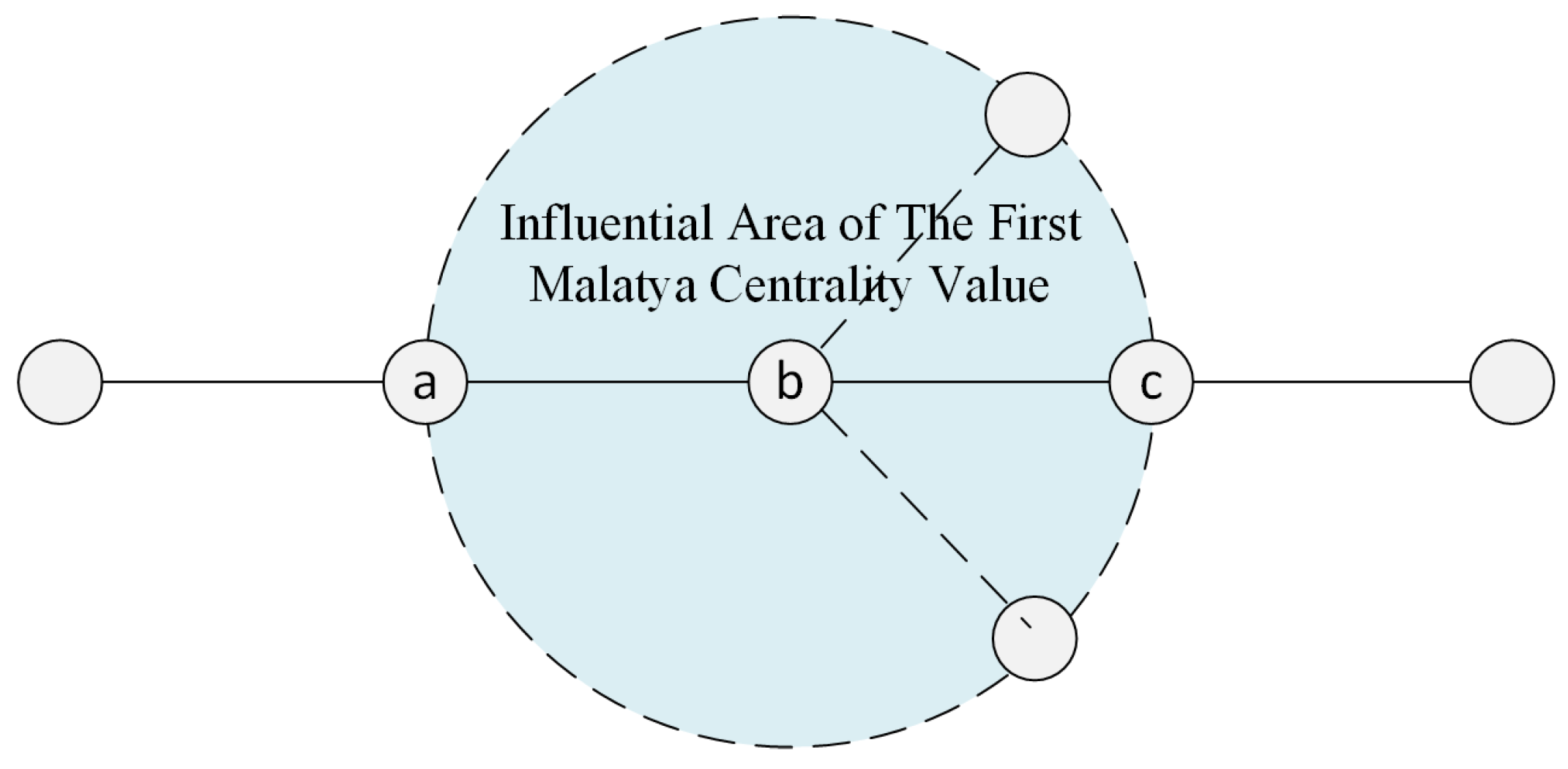
4.1. The First Malatya Centrality Value

The Malatya centrality algorithm uses node values that calculate the strength of the nodes of the given graph relative to each other and the result value is called Malatya centrality value. A basic principle used in this paper is at this aim.

Principle 1.

The strength of an entity should be given as the relative strength it has relative to the strength of its neighbors in its society.

The strength of the nodes of the given graph can be calculated and Definition 3 is given for this purpose based on Principle 1. This definition consists of calculating the centrality value of each node and then multiplying the resulting value by the ratio of the active degree to the node degree. In the first step, the active node degree is equal to the node degree, therefore the ratio will be equal to one. Active node degree is the number of neighbors of a node that are white nodes (initially, all nodes of graph are regarded as white nodes that indicate where it is not yet clear whether nodes belong to the dominating set or belong to the neighbor set).

Definition 3.

Assume that $G=(V,E)$ is a graph and $\forall v_i\in V$, set $V_N\left(v_i\right)$ is the set of neighbors of the node $vi, \forall \mathit{vi}\in V$.

$${\Psi }_1\left(v_i\right)={\displaystyle \frac{d_a\left(v_i\right)}{d\left(v_i\right)}}\left({\sum }_{v_i\in V,v_j\in V_N\left(v_i\right)}{\displaystyle \frac{d\left(v_i\right)}{d\left(v_j\right)}}\right)$$

(2)

The obtained value ${\Psi }_1$ is called the first Malatya centrality value of node v_i where $d\left(v_i\right)$ is the degree of node $v_i$, and $d_a\left(v_i\right)$ is the active degree of $v_i$ where active degree is the number of white neighbors of related node (the related node in Equation (2) is $v_i,1\le i\le n$).

The centrality value of each node is calculated by using the equation in 2, and this value is based on the logic of Principle 1. In this way, it concludes in the calculation of a node’s strength relative to its neighbors (the calculation of a node’s strength relative to its neighbor is inversely proportional to the degree of the relevant node). The algorithms can be constructed to find solutions for Maximum Independent Set and Minimum Node-Cover problems in the given graph by using the first Malatya centrality values. The steps to calculate the first Malatya centrality are given in Algorithm 1, with pseudo-codes.

Algorithm 1. The First Malatya Centrality Algorithm.

function FirstMalatyaCentrality (A, D, DA) output: MC1//The first Malatya centrality values input: A, //Adjacency matrix      D, //Degree vector      DA //Active degree vector 1 for i ← 1…n  //(A is of sizes n × n) 2  L ← Neighbors(i) 3  for j in L 4   MC1(i) = MC1(i) + D(i)/D(j) 5  end 6 end 7 MC1 = MC1*DA //vector inner product 8 for i ← 1,…,n 9  if D(i) ≠ 0 10   MC1(i) = MC1(i)/D(i) 11  end 12 end 13 return MC1

The impact area of the first Malatya centrality value on the graph is given in Figure 1. The centrality value of each node is calculated according to the nodes directly connected to it. The first Malatya centrality value shows the logic of calculating the relative strength of a node relative to its neighbors. Assuming we want to compute the first centrality value of node ‘b’, the nodes ‘a’, ‘c’, and dashed nodes should be taken into consideration since nodes one step away are taken into consideration for computing the first Malatya centrality values. All nodes are one step far away from the ‘b’ node, these nodes are regarded as in the first Malatya centrality influential area (region). The First Malatya centrality value of a node involves using the degrees of nodes one step away from that node.

Figure 1. The influential area of the first Malatya centrality values.

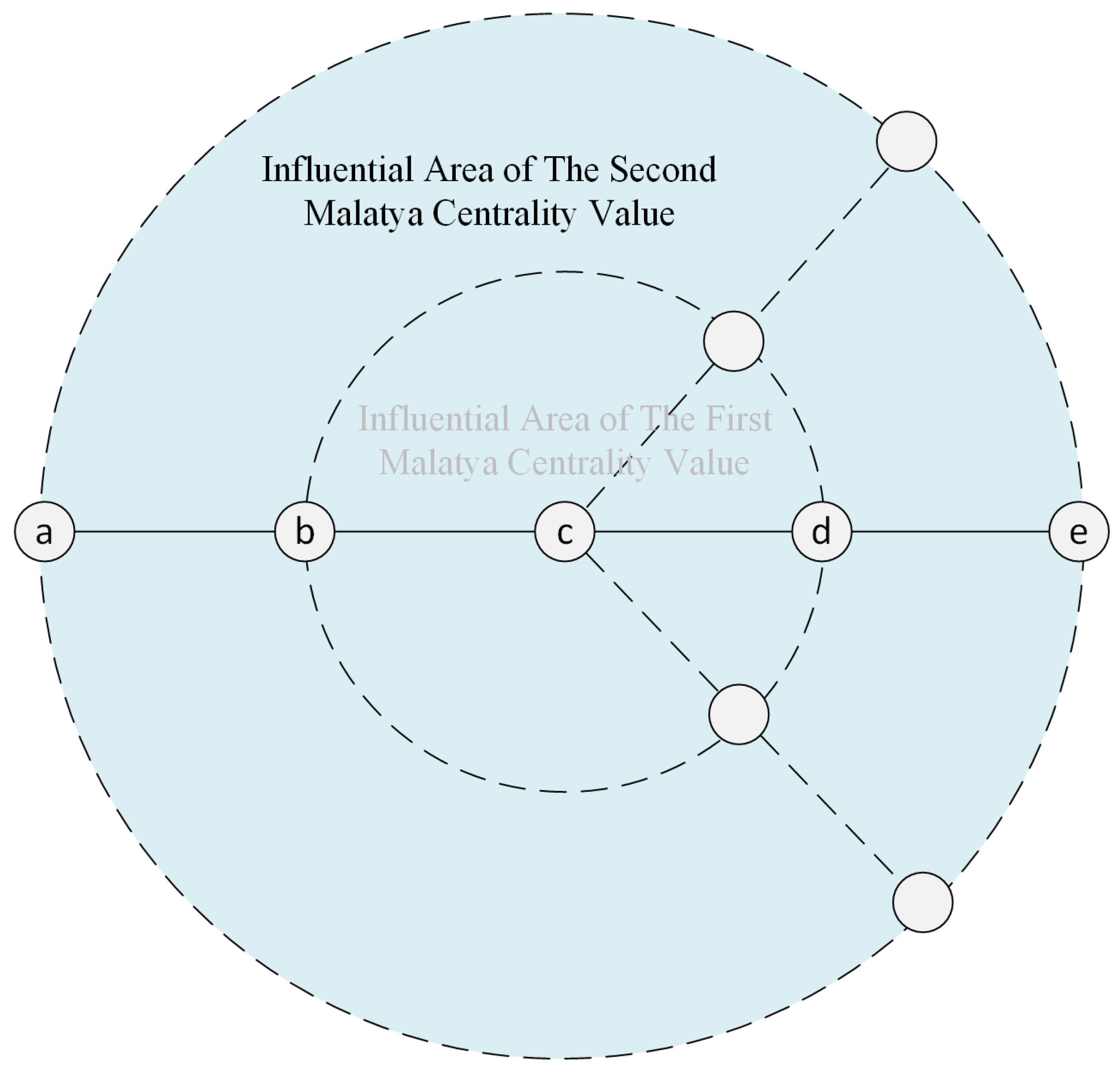
4.2. The Second Malatya Centrality Value

The previous section describes the method for calculating the first Malatya centrality value. The logic of calculating this value is based on the logic that the degree of a node can be computed according to the degrees of the neighbors of the corresponding node. The first Malatya centrality value reveals the status of a node relative to its neighbors. The obtained value is also called the relative strength of the corresponding node.

The second stage centrality value, which is similar to the first Malatya centrality logic, can be calculated because a node’s neighbors are also involved for the sake of the dominating set, not just its own neighbors. The second principle can be put forward based on this logic.

Principle 2.

The relative strength of an entity can be given as the relative strength it has relative to the relative strength of its neighbors in its society.

The second-level strength of the node can be obtained by using this principle, and Definition 4 is given for this reason.

Definition 4.

Assume that  $G=(V,E)$  is a graph and  $\forall v_i\in V$  except selected nodes,  $V_N\left(v_i\right)$  is the set of neighbors of node  $v_i, v_i\in V.$

$${\Psi }_2\left(v_i\right)={\displaystyle \frac{1}{d\left(v_i\right)}}{\displaystyle \frac{d_a\left(v_i\right)}{d\left(v_i\right)}}\left({\sum }_{v_i\in V,v_j\in V_N\left(v_i\right)}{\displaystyle \frac{{\Psi }_1\left(v_i\right)}{{\Psi }_1\left(v_j\right)}}\right)$$

(3)

The obtained value ${\Psi }_2$ is called the second Malatya centrality value of node u where $d\left(v_i\right)$ is the degree of node $v_i$, and $d_a\left(v_i\right)$ is the active degree of vi where active degree is the number of white neighbors of related node (the related node in Equation (3) is $v_i,1\le i\le n$).

The centrality value of each node is calculated with the correlation given in Definition 4, and this value is based on the logic of Principle 2. In this way, it reveals the calculation of the relative strength of a node compared to its neighbors. Initially, all nodes are designated as “white” nodes, and when a node is selected for the dominating set, the neighbors of that node are marked as “grey” nodes where a grey node does not belong to the dominating set and it has at least one neighbor node in the dominating set.

This paper aims to calculate the second Malatya centrality value and obtain the MDS. Therefore, a two-stage centrality value or relative strength was calculated. The impact area (influential area) of the second Malatya centrality value is given in Figure 2. Since this paper aims to obtain the MDS in the given graph, the domain of the relative strength must be at least as shown in Figure 2. For example, when node 2 is included in the dominating set, node 3 is not included in the dominating set because it is adjacent to the selected node. To minimize the number of elements in the dominating set, node 4 is not included and node 5 may be included in the dominating set concerning the given graph in Figure 2. Algorithm 2 illustrates the pseudo-code of algorithm computing the second Malatya centrality values.

Figure 2. The influential area of the second Malatya centrality values.

Assume that the aim is to compute the second Malatya centrality value for node ‘c’. The nodes ‘b’ and ‘d’ and the dashed nodes on the inner circle are taken into consideration for computing the first Malatya centrality value for node ‘c’. This process is carried on for all nodes. The next step is to compute the second Malatya centrality value. All nodes two steps far away from node ‘c’ are taken into consideration for computing the second Malatya centrality value of node ‘c’ as seen in Equation (3) (Definition 4). To consider nodes two steps far away, the first Malatya centrality values should be used as similar to degree usage (as seen in Equation (2), Definition 1). To calculate the second Malatya centrality value of a node, the first Malatya centrality values of the neighbors of the related node are used. This means that since the degrees of nodes that are one step away are used in the first Malatya centrality value, using the first Malatya centrality value in computing the second Malatya centrality value means that all nodes that are two steps away are included in the computation (Figure 2).

Algorithm 2. The Second Malatya Centrality Algorithm

function SecondMalatyaCentrality (A, D, DA, MC1, MC2) output: MC2  //The second Malatya centrality values input: A,  //Adjacency matrix 1 for i ← 1…n //(A is of sizes n × n) 2  L ← Neighbors(i) 3  for j in L 4   MC1(i) = MC1(i) + D(i)/D(j) 5  end 6 end 7 MC1 = MC1*DA 8 for i ← 1, …, n 9  if D(i) ≠ 0 10   MC1(i) = MC1(i)/D(i) 11  end 12 end 13 return MC1

4.3. The Main Algorithm

The dominating set determination is handled by the sequence of applications of centrality values computation. In the first step, the node with the maximum second Malatya centrality value is selected and removed from the graph. Its neighbors are designated as grey nodes, and the white neighbors of any node designate the active degree of the corresponding node. The grey nodes with active degrees equal to 1 are also removed from the graph. Algorithm 3 illustrates the pseudo-code of the dominating set algorithm. The function NodeSelection (A, D, DA, NodeColor, MC2, VD) selects a node with the maximum second Malatya centrality value for the dominating set, and then it removes this node from the graph. The neighbors of the selected node are marked as grey nodes. The grey nodes with active degree as 1 are also removed from the graph. If a grey node has maximum MC2 and its white neighbor’s number is greater than the white neighbors of any white node with maximum MC2 amongst white nodes, then this grey node is selected for the dominating set. Otherwise, the white node with maximum MC2 is selected for the dominating set.

Algorithm 3. The Dominating Set Algorithm

function DominatingSet (A) output: VD ← ∅ input:  A,  //Adjacency matrix 1 n ← sizeof(A)  //n is the size of graph (G = (V,E), |V| = n) 2 MC1 ← 0, MC2 ← 0 3 NodeColor ← 0  //Grey node = 1, White nod e = 0 4 D ← ∅  //Degree vector 5 DA ← ∅ //Active degree vector 6 NodeColor(G) ← white 7 while Termination ≠ False 8  MC1 ← FirstMalatyaCentrality (A, D, DA, MC1) 9  MC2 ← SecondMalatyaCentrality (A, D, DA, MC1, MC2) 10  NodeColor ← NodeSelection (A, D, DA, NodeColor, MC2) 11  Termination ← Terminate (A, NodeColor) 12 End 13 return VD 14 function NodeSelection (A, D, DA, NodeColor, MC2, VD) 15  SN ← Max (MC2) //Select the node with the maximum MC2 value (white node has priority) 16  NodeColor (SN) ← red 17  NodeColor (Neighbors of SN) ← grey 18  return NodeColor 19 function Terminate (A, NodeColor) 20  n ← sizeof (A) 21  Termination ← false; 22  for i ← 1, …, n 23   if NodeColor (i) is white 24    Termination ← true 25   end 26  end 27  return Termination

Theorem 1.

Assume that  $G=(V,E)$  is a graph where  $\left|V\right|=n$  and  $\left|E\right|=m$. Algorithm 1 has polynomial time and space complexities.

Proof. 

The proof of theorem can be given in two ways:

• First Way: Adjacency matrix method.
  Space: The adjacency matrix of given graph is used and the proposed algorithm is an iterative algorithm not a recursive algorithm. Consequently, the space complexity is $O(n\times d)$, where $\left|V\right|=n$ and d is the average degree. Thus, the space complexity of Algorithm 1 is $P_{MC1}\left(n\right)=\mathsf{\Theta }(n\times d)$.
  Time: Assume that $G=(V,E)$ and its adjacency matrix is $A$ of size $nxn$. To compute the first round ${\Psi }_1\left(\dots \right)$ values, an adjacency matrix $A$ of $G$ is used, and it requires $O(n\times d)$ time complexity, since the adjacency matrix has size $nxn$ and the average degree is d. That is why the time complexity of Algorithm 1 is $T_{MC1}\left(n\right)=\mathsf{\Theta }(n\times d)$.
• Second Way: Linked list method using neighbors list.
  Space: The neighbors of any node are stored as a linked list data structure. Assume that the averaged degree in graph $G$ is $\Delta \left(G\right)$. If $\left|V\right|=n$, the space complexity of Algorithm 1 is $P_{MC1}\left(n\right)=\mathsf{\Theta }(\mathrm{n}.\Delta \left(\mathrm{G}\right))$.
  Time: If linked list data structures are used to represent the given graph, the space requirement for storing graph is $\Delta \left(G\right)\times n$. The time complexity of each node to compute ${\Psi }_1\left(\dots \right)$ is maximum $\Delta \left(G\right)$. There are $n$ nodes, and so, the time complexity of Algorithm 1 is $O(\Delta (G)\times n)$. □

Theorem 2.

Assume that $G=(V,E)$ is a graph where $\left|V\right|=n$ and $\left|E\right|=m$. Algorithm 2 has polynomial time and space complexities.

Proof. 

Proceeding analogously as in the proof of Theorem 1, similar results yield. □

Theorem 3.

Assume that $G=(V,E)$ is a graph where $\left|V\right|=n$ and $\left|E\right|=m$. DominatingSet algorithm has polynomial time and space complexities.

Proof. 

Assume that $G=(V,E)$ and its adjacency matrix is A of size $\mathrm{n}\mathrm{x}\mathrm{n}$. In the first step, ${\Psi }_1\left(\dots \right)$ and ${\Psi }_2\left(\dots \right)$ are computed. The arrays ${\Psi }_1\left(\dots \right)$ and ${\Psi }_2\left(\dots \right)$ are 1-dimensional arrays, and the searching process for selecting a node for the dominating set takes place and its time complexity is $T_S\left(n\right)=O\left(n\right)$. After selecting one node for the dominating set this node is removed from the graph. After removing the selected node ($u_1$), the graph is updated, and so

$G_1=G-\left\{u_1\right\}$ where $G_1=(V_1,E_1)$ where $V_1\subset V$ and $E_1\subset E$.

For the second node selection process, Algorithms 1 and 2 are used to compute the centrality values of G1. Then, selecting the next node for the dominating set is a linear process, and the selected node ($u_2$) is also removed from the graph. Then the graph is updated again.

$G_2=G_1-\left\{u_2\right\}$ where $G_2=(V_2,E_2)$ where $V_2\subset V_1$ and $E_2\subset E_1$.

This process continues this way until $G_{\mathsf{\gamma }\left(G\right)}$ contains all grey nodes or null graphs where $\mathsf{\gamma }\left(G\right)$ is the domination number of graphs is the cardinality of the dominating set. So, the sequence of graph updating is:

$G_1=G-\left\{u_1\right\}$, where $G_1=\left(V_1,E_1\right),$ where $V_1\subset V$ and $E_1\subset E$.

$G_2=G_1-\left\{u_2\right\}$, where $G_2=(V_2,E_2)$ where $V_2\subset V_1$ and $E_2\subset E_1$.

$G_3=G_2-\left\{u_3\right\}$, where $G_3=(V_3,E_3)$ where $V_3\subset V_2$ and $E_3\subset E_2$.

………………

$G_{\mathsf{\gamma }}\left(G\right)=G_{\mathsf{\gamma }}\left(G\right)-1-\left\{u_{\mathsf{\gamma }}\right(G\left)\right\}$ where $G_{\mathsf{\gamma }\left(G\right)}=(V_{\mathsf{\gamma }\left(G\right)},E_{\mathsf{\gamma }\left(G\right)})$ where $V_{\mathsf{\gamma }\left(G\right)}\subset V_{\mathsf{\gamma }\left(G\right)-1}$ and $E_{\mathsf{\gamma }\left(G\right)}\subset E_{\mathsf{\gamma }\left(G\right)-1}$.

The time complexity of dominating set algorithm is:

Case 1: Adjacency matrix, and $\gamma \left(G\right)$ is the cardinality of dominating set, $T_S(\dots )$ is the time searching node for dominating set.

$$\begin{array}{c}{T}_{DS}\left(n\right)=\underset{\gamma \left(G\right)}{\underbrace{\begin{array}{c}\stackrel{1^{st}step}{\overbrace{T_{MC1}\left(n\right)+T_{MC2}\left(n\right)+T_S\left(n\right)}}+\stackrel{2^{nd}step}{\overbrace{T_{MC1}\left(n_1\right)+T_{MC2}\left(n_1\right)+T_S\left(n_1\right)}}+\cdots \\ +\stackrel{{\gamma \left(G\right)}^{th}step}{\overbrace{T_{MC1}\left(n_{\gamma \left(G\right)-1}\right)+T_{MC2}\left(n_{\gamma \left(G\right)-1}\right)+T_S\left(n_{\gamma \left(G\right)-1}\right)}}\end{array}}}\\ =\underset{\gamma \left(G\right)}{\underbrace{\begin{array}{c}\stackrel{1^{st}step}{\overbrace{\mathsf{\Theta }\left(n\times d\right)+\mathsf{\Theta }\left(n\times d\right)+O\left(n\right)}}+\stackrel{2^{nd}step}{\overbrace{\mathsf{\Theta }\left(n_1\times d\right)+\mathsf{\Theta }\left(n_1\times d\right)+O\left(n_1\right)}}+\cdots \\ +\stackrel{{\gamma \left(G\right)}^{th}step}{\overbrace{\mathsf{\Theta }\left(n_{\gamma \left(G\right)-1}\times d\right)+\mathsf{\Theta }\left(n_{\gamma \left(G\right)-1}\times d\right)+O\left(n_{\gamma \left(G\right)-1}\right)}}\end{array}}}\\ =\mathrm{O}\left(\gamma \left(G\right)(n\times d)\right)\end{array}$$

The time complexity of DominatingSet algorithm is bounded by a polynomial, and the space complexity of DominatingSet algorithm is also O($n\times d$) as Algorithms 1 and 2.

Case 2: Linked list

$$\begin{array}{c}{T}_{DS}\left(n\right)=\underset{\gamma \left(G\right)}{\underbrace{\begin{array}{c}\stackrel{1^{st}step}{\overbrace{T_{MC1}\left(n\right)+T_{MC2}\left(n\right)+T_S\left(n\right)}}+\stackrel{2^{nd}step}{\overbrace{T_{MC1}\left(n_1\right)+T_{MC2}\left(n_1\right)+T_S\left(n_1\right)}}+\cdots \\ +\stackrel{{\gamma \left(G\right)}^{th}step}{\overbrace{T_{MC1}\left(n_{\gamma \left(G\right)-1}\right)+T_{MC2}\left(n_{\gamma \left(G\right)-1}\right)+T_S\left(n_{\gamma \left(G\right)-1}\right)}}\end{array}}}\\ =\underset{\gamma \left(G\right)}{\underbrace{\begin{array}{c}\stackrel{1^{st}step}{\overbrace{\mathsf{\Theta }\left(∆\left(G\right)\times n\right)+\mathsf{\Theta }\left(∆\left(G\right)\times n\right)+O\left(n\right)}}+\stackrel{2^{nd}step}{\overbrace{\mathsf{\Theta }\left(∆\left(G\right)\times n_1\right)+\mathsf{\Theta }\left(∆\left(G\right)\times n_1\right)+O\left(n_1\right)}}+\cdots \\ +\stackrel{{\gamma \left(G\right)}^{th}step}{\overbrace{\mathsf{\Theta }\left(∆\left(G\right)\times n_{\gamma \left(G\right)-1}\right)+\mathsf{\Theta }\left(∆\left(G\right)\times n_{\gamma \left(G\right)-1}\right)+O\left(n_{\gamma \left(G\right)-1}\right)}}\end{array}}}\\ =\mathrm{O}\left(\gamma \left(G\right)\times n\times ∆\left(G\right)\right)\end{array}$$

So, the proof of complexity is completed. □

5. Experimental Results

The experimental results will be shown on some small graphs, and the experimental results on large graphs will be shown as tabulated.

Example 1.

The first example is a grid $G=(V,E)$ where $\left|V\right|=n$. An example of a $5\times 6$ grid graph is shown in Figure 3.

Figure 3. A grid of size 5 × 6.

According to the centrality values, Table 1 shows that the nodes with the potential to be selected are 2, 4, 6, 10, 21, 25, 27, and 29. In this step, the method selected node 6 and removed it from the graph. After the deletion process was completed, node 1 became a grey node and its active degree was dropped to 1. Therefore, this node was also removed from the graph. This situation is seen in Figure 4 (first step).

Table 1. Centrality values for the first step.

Node #	1	2	3	4	5	6	7	8	9	10	11	12	13	14	15
Ψ1	1.33	3.25	2.75	3.25	1.33	3.25	4.67	4.33	4.67	3.25	2.75	4.33	4	4.33	2.75
Ψ2	0.41	1.44	0.77	1.44	0.41	1.44	1.26	1.13	1.26	1.44	0.83	1.15	0.94	1.15	0.83
Node #	16	17	18	19	20	21	22	23	24	25	26	27	28	29	30
Ψ1	2.75	4.33	4	4.33	2.75	3.25	4.67	4.33	4.67	3.25	1.33	3.25	2.75	3.25	1.33
Ψ2	0.83	1.15	0.94	1.15	0.83	1.44	1.26	1.13	1.26	1.44	0.41	1.44	0.78	1.44	0.41

Note: Bold text indicates the nodes with the highest centrality values.

Figure 4. Application steps of Malatya Dominating Set Algorithm to grid of sizes 5 × 6. Red nodes represent the nodes included in the dominating set. Gray nodes are nodes that are neighbors to a dominating set node. Blue nodes indicate nodes that have not yet been visited.

Node 3 has the maximum Ψ2 according to Table 2, and this node is selected and removed from the graph. The status of neighbors of node 3 turned grey (these are 2, 4, 8). The corresponding graph is seen in Figure 4 in the second step. The node with maximum Ψ2 is 10 (Table 3), and it was selected to dominating set and node 10 was removed from the graph (the resultant graph is seen in Figure 4, third step).

Table 2. Centrality values for the second step.

Node #	1	2	3	4	5	6	7	8	9	10	11	12	13	14	15
Ψ1	0	0.67	3.25	3.25	1.33	0	3	3.50	4.67	3.25	1.17	2.67	4	4.33	2.75
Ψ2	0	0.11	2.27	1.38	0.41	0	2.16	0.73	1.32	1.44	0.49	0.56	1.14	1.15	0.83
Node #	16	17	18	19	20	21	22	23	24	25	26	27	28	29	30
Ψ1	2.17	4.33	4	4.33	2.75	3.25	4.67	4.33	4.67	3.25	1.33	3.25	2.75	3.25	1.33
Ψ2	0.67	1.41	0.94	1.15	0.83	1.55	1.26	1.13	1.26	1.44	0.41	1.44	0.78	1.44	0.41

Note: Bold text indicates the nodes with the highest centrality values.

Table 3. Centrality values for the third step.

Node #	1	2	3	4	5	6	7	8	9	10	11	12	13	14	15
Ψ1	0	0	0	1.50	0.83	0	0	1	3.17	3.25	1.33	2	4	4.33	2.75
Ψ2	0	0	0	1.14	0.20	0	0	0.28	0.87	2.04	0.64	0.54	1.48	1.26	0.83
Node #	16	17	18	19	20	21	22	23	24	25	26	27	28	29	30
Ψ1	2.17	4.67	4	4.33	2.75	3.25	4.67	4.33	4.67	3.25	1.33	3.25	2.75	3.25	1.33
Ψ2	0.61	1.66	0.93	1.15	0.83	1.55	1.24	1.13	1.26	1.44	0.41	1.44	0.78	1.44	0.41

Note: Bold text indicates the nodes with the highest centrality values.

Table 4 illustrates that the nodes with the maximum Ψ2 are node 17 and node 19. Malatya Dominating Set Algorithm selected node 19, and it removed this node from the graph (the resultant graph is seen in Figure 4, third step). The fifth step’s centrality values are seen in Table 5. Node 24 has the maximum centrality value; however, it is a grey node and its contribution to the dominating set is less than node 21 whose centrality value is maximum amongst the white nodes. Due to this case, node 21 was selected and it was removed from the graph (the resultant graph is seen in Figure 4, fifth step).

Table 4. Centrality values for the fourth step.

Node #	1	2	3	4	5	6	7	8	9	10	11	12	13	14	15
Ψ1	0	0	0	0	0	0	0	0	0	0	1.33	2.17	2.75	2.17	1.33
Ψ2	0	0	0	0	0	0	0	0	0	0	0.62	0.64	1.06	0.64	0.62
Node #	16	17	18	19	20	21	22	23	24	25	26	27	28	29	30
Ψ1	2.17	4.67	4.33	4.67	2.17	3.25	4.67	4.33	4.67	3.25	1.33	3.25	2.75	3.25	1.33
Ψ2	0.61	1.60	1.11	1.60	0.61	1.55	1.24	1.11	1.24	1.55	0.41	1.44	0.78	1.44	0.41

Note: Bold text indicates the nodes with the highest centrality values.

Table 5. Centrality values for the fifth step.

Node #	1	2	3	4	5	6	7	8	9	10	11	12	13	14	15
Ψ1	0	0	0	0	0	0	0	0	0	0	1.33	2.50	0.67	0	0
Ψ2	0	0	0	0	0	0	0	0	0	0	0.58	1.40	0.12	0	0
Node #	16	17	18	19	20	21	22	23	24	25	26	27	28	29	30
Ψ1	2.17	3.75	3	0	0	3.25	4.67	2.50	3.25	0.83	1.33	3.25	2.75	2.33	1.67
Ψ2	0.64	1.00	2.17	0	0	1.55	1.50	0.38	2.20	0.19	0.41	1.44	1.04	0.66	1.36

Note: Bold text indicates the nodes with the highest centrality values.

The remaining steps of the algorithm are as follows: In the sixth step, node 28 was selected and its neighbors are 23, 27, and 29. The seventh step concluded in the selection of node 12 with neighbors 7, 11, 13, and 17. The last step concluded with the selection of node 25 with neighbors 20, 24, and 30. After this step, there will be no white nodes.

Example 2.

This example includes the application of the Malatya Dominating Set Algorithm to Banana Tree graph.

The centrality values are obtained when the algorithm is run on the graph seen in Figure 5, and the centrality values are seen in Table 6. The nodes with maximum centrality values are 6, 12, and 18. The algorithm selected node 6, and the resultant graph is seen in Figure 6.

Figure 5. Banana tree.

Table 6. Centrality values for Banana Tree graph at the first step.

Node #	1	2	3	4	5	6	7	8	9	10
Ψ1	1.07	0.2	0.2	0.2	0.2	22.5	1.07	0.2	0.2	0.2
Ψ2	0.14	0.009	0.009	0.009	0.009	94.22	0.14	0.009	0.009	0.009
Node #	11	12	13	14	15	16	17	18	19
Ψ1	0.2	22.5	1.07	0.2	0.2	0.2	0.2	22.5	4.5
Ψ2	0.009	94.22	0.14	0.009	0.009	0.009	0.009	94.22	4.22

Note: Bold text indicates the nodes with the highest centrality values.

Figure 6. Results of the algorithm’s first iteration on banana tree. (a) The raw output of the graph generated by the algorithm (b) Readable visualization of the graph.

The nodes that have the potential to be selected according to the centrality values given in Table 7 are nodes 12 and 18. After the selection of node 12, nodes 7, 8, 9, 10, and 11 are neighbors of the selected node and they are removed from the graph due to the active degrees.

Table 7. Centrality values for Banana Tree graph at the second step.

Node #	1	2	3	4	5	6	7	8	9	10
Ψ1	0	0	0	0	0	0	1.4	0.2	0.2	0.2
Ψ2	0	0	0	0	0	0	0.38	0.009	0.009	0.009
Node #	11	12	13	14	15	16	17	18	19
Ψ1	0.2	22.5	1.4	0.2	0.2	0.2	0.2	0.2	22.5
Ψ2	0.009	93.21	0.38	0.009	0.009	0.009	0.009	93.21	1.43

Note: Bold text indicates the nodes with the highest centrality values.

The obtained result graph is seen in Figure 7a. The next step of algorithm obtained the node 18 having the maximum second Malatya centrality value. Then, this node is selected and removed from the graph. Finally, node 19 will remain as an isolated node and this is also added to the dominating set.

Figure 7. The resultant graphs of second (a) and third (b) iterations.

Example 3.

The last step for experimental studies contains large graph applications. To this aim, there are 10 graphs that were used for experimental studies. The applications for large graphs are given in Table 8 and Table 9. These studies were carried out on a computer with Intel Core i7-10875H processor, 2.30 GHz, and 32 GB RAM.

Table 8. The experimental results for large graphs.

Dataset	Number of Nodes	Number of Edges	Dominating Set	Time (S)
Random generated graph	70	133	VD = {1, 7, 10, 16, 23, 26, 32, 36, 37, 39, 44, 47, 52, 56, 65, 67}	0.051
dsjc250.5 [41]	250	31,336	VD = {1, 62, 87, 118, 189}	0.041
dsjc500.1 [41]	500	12,458	VD = {32, 40, 55, 56, 70, 101, 150, 160, 164, 201, 204, 205, 211, 247, 256, 295, 312, 332, 337, 349, 390, 405, 494}	0.091
latin_square [42]	900	307,350	VD = {1, 721}	0.107
flat1000_50_0 [42]	1000	245,000	VD = {266, 326, 357, 672, 704, 969}	0.175
r1000.5 [43]	1000	238,267	VD = {13, 241, 374, 483, 602}	0.095
dsjc1000.1 [41]	1000	49,629	VD = {12, 22, 65, 120, 166, 184, 207, 253, 317, 382, 387, 394, 523, 531, 565, 618, 627, 638, 651, 676, 741, 768, 793, 813, 855, 870, 950}	0.219
C2000.5 [42]	2000	999,836	VD = {17, 545, 552, 636, 826, 1023, 1324}	0.745
flat1000_60_0 [42]	1000	245,830	VD = {41, 60, 475, 747, 748, 966}	0.204
flat1000_76_0 [42]	1000	246,708	VD = {171, 467, 508, 531, 550, 595}	0.125

Table 9. The comparison result on BHOSLIB datasets.

Dataset	CC2FS [44]	FastMWDS [25]	RLS0 [17]	ScBppw [26]	FastDS [27]	Our Work
frb40-19-1 [45]	14	14	14	15	14	2
frb40-19-2 [45]	14	14	15	16	14	2
frb40-19-3 [45]	14	14	15	16	14	2
frb40-19-4 [45]	14	14	15	15	14	2
frb40-19-5 [45]	14	14	15	15	14	2
frb45-21-1 [45]	16	16	16	17	16	2
frb45-21-2 [45]	16	16	17	18	16	2
frb45-21-3 [45]	16	16	17	17	16	2
frb45-21-4 [45]	16	16	17	17	16	2
frb45-21-5 [45]	16	16	17	18	16	2
frb50-23-1 [45]	18	18	19	19	18	2
frb50-23-2 [45]	18	18	19	19	18	2
frb50-23-3 [45]	18	18	19	20	18	2
frb50-23-4 [45]	18	18	20	19	18	2
frb50-23-5 [45]	18	18	19	19	18	2
frb53-24-1 [45]	19	19	20	21	19	2
frb53-24-2 [45]	19	19	20	21	19	2
frb53-24-3 [45]	19	19	20	20	19	2
frb53-24-4 [45]	18	19	19	19	18	2
frb53-24-5 [45]	19	19	20	20	19	2
frb56-25-1 [45]	20	20	21	21	20	2
frb56-25-2 [45]	20	20	21	21	20	2
frb56-25-3 [45]	20	20	22	21	20	2
frb56-25-4 [45]	20	20	22	22	20	2
frb56-25-5 [45]	20	20	21	21	20	2
frb59-26-1 [45]	21	21	22	22	20	2
frb59-26-2 [45]	21	21	22	22	21	2
frb59-26-3 [45]	21	21	22	23	21	2
frb59-26-4 [45]	21	21	23	23	21	2
frb59-26-5 [45]	21	21	24	23	21	2
frb100-40 [45]	37	38	40	39	36	2
Average Run Time	96.68 s	101.44 s		-	95.62 s	0.761 s

Note: Bolds are the best results for datasets.

Table 8 presents the experimental results for large graphs, highlighting the performance of the MDSA on datasets of varying sizes. The table includes data on the number of nodes and edges, the size of the dominating set found (VD), and the execution time in seconds.

In Table 8:

• Random Generated Graph: The algorithm identified a dominating set of 15 nodes out of 70 nodes with 133 edges, completing the task in 0.051 s.
• dsjc500.1: For this graph with 500 nodes and 12,458 edges, MDSA found a dominating set of 23 nodes, executing in 0.091 s.
• latin_square: With 900 nodes and 307,350 edges, MDSA found a dominating set of 2 nodes, taking 0.107 s.
• flat1000_50_0: This graph contains 1000 nodes and 245,000 edges. MDSA identified a dominating set of 6 nodes in 0.175 s.
• dsjc250.5: For this graph with 250 nodes and 31,336 edges, MDSA found a dominating set of 5 nodes, executing it in 0.041 s.
• r1000.5: This graph has 1000 nodes and 238,267 edges. MDSA identified a dominating set of 5 nodes in 0.095 s.
• dsjc1000.1: For this graph containing 1000 nodes and 49,629 edges, MDSA found a dominating set of 27 nodes, executing it in 0.219 s.
• C2000.5: For this graph with 2000 nodes and 999,836 edges, MDSA identified a dominating set of 7 nodes, completing in 0.745 s.
• flat1000_60_0: This dataset has 1000 nodes and 245,830 edges, with MDSA finding a dominating set of 7 nodes in 0.204 s.
• flat1000_76_0: With 1000 nodes and 246,708 edges, MDSA found a dominating set of 6 nodes, executing it in 0.125 s.

The experimental results demonstrate that the proposed algorithm effectively applies the principles of both the greedy search algorithm and dynamic programming. At each step, the algorithm utilizes the Malatya centrality value as the selection criterion for adding a node to the dominating set. This ensures that the most central node, based on the degrees of its neighboring nodes, is consistently selected. The dynamic nature of the algorithm is evident as it recalculates the Malatya centrality values whenever a node is selected, reflecting the changes in the degrees of its neighboring nodes. This process of storing and reusing the results of subproblems allows for the algorithm to avoid unnecessary computations and maintain high efficiency. The performance metrics in our experiments show that the algorithm selects the optimal nodes efficiently, underscoring its practical applicability and effectiveness in solving the minimum dominating set problem across various graph structures and sizes.

The results presented in Table 9 reveal that the Malatya Dominating Set Algorithm (MDSA) outperforms other existing algorithms for the BHOSLIB datasets. MDSA achieved the smallest dominating set sizes (2) among all algorithms for these datasets. Additionally, the execution times were significantly shorter (0.761 s) compared to others. Furthermore, these results were performed using a computer with lower hardware capacity than other studies. These results demonstrate that MDSA provides efficient and rapid solutions, especially for large datasets, indicating its adaptability to a wide range of applications and its potential use in solving other NP-hard problems.

Table 10 includes a comparison of MDSA with other existing algorithms on large-scale network datasets. The performance metric used is the minimum dominating set (D_min) values. MDSA has determined smaller or equal D_min values in many datasets compared to other algorithms. However, FastDS has shown the best performance across all benchmarks included in this table. When considering time complexity, MDSA is superior. FastDS consists of two main phases. The first phase, the local search process, has an average time complexity of $\Theta (n\times logn)$, where n is node size. The second phase involves the application of inference rules, which has a time complexity of $\Theta \left(m\right)$, where m is edge size. In total, the time complexity of FastDS is expressed as $\Theta (n\times logn+m)$. For MDSA, Algorithms 1 and 2 operate only among the neighbors for each node, resulting in a total time complexity of $\Theta (n\times d)$, and it has a simpler and faster growth rate. FastDS, with a time complexity of $\Theta (n\times logn+m)$, has a more complex growth rate, especially due to the $n\times logn$ term. This is more evident when looking at the average execution times in Table 9.

Table 10. The comparison results of D_min values for big networks.

Dataset	FastMWDS [25]	RLS0 [17]	ScBppw [26]	FastDS [27]	Our Work
Amazon0302 [46]	35,616	38,735	36,199	35,593	37,806
Amazon0312 [46]	45,531	49,326	45,914	45,490	47,424
Amazon0505 [46]	47,362	51,281	47,734	47,310	49,207
Amazon0601 [46]	42,319	45,952	42,717	42,289	44,274
Cit-HepPh [47]	3078	3192	3087	3078	3223
Cit-HepTh [47]	2935	2985	2944	2936	3023
Email-EuAll [46]	18,181	18,181	18,181	18,181	18,179
p2p-Gnutela04 [47]	2227	2227	2227	2227	2239
p2p-Gnutela24 [47]	5418	5418	5418	5418	5418
p2p-Gnutela25 [47]	4519	4519	4519	4519	4519
p2p-Gnutela30 [47]	7169	7169	7169	7169	7169
p2p-Gnutela31 [47]	12,582	12,593	12,582	12,582	12,582
soc-Slashdot0811 [48]	14,312	14,333	14,312	14,312	14,323
soc-Slashdot0902 [48]	15,305	15,334	15,305	15,305	15,351
soc-Epinions1 [49]	15,734	15,742	15,734	15,734	15,751
web-BerkStan [48]	28,434	30,119	28,615	28,432	28,972
web-Google [48]	79,700	81,106	79,756	79,699	80,334
web-NotDame [50]	23,733	23,950	23,746	23,735	23,800
web-Stanford [48]	13,198	14,099	13,298	13,199	13,433
Wiki-Vote [3]	1116	1116	1116	1116	1116
cond-mat-2005 [51]	6508	6509	6531	6508	5748

Note: Bolds are the best results for datasets.

To demonstrate the strengths of the proposed algorithm, another comparison result is presented in Table 11. This comparison example includes the greedy algorithm, the CBC algorithm from [24], and the RLSo algorithm from [17]. Unlike our proposed algorithm, these studies employ heuristic approaches and therefore rely on repeated runs to obtain the optimal result. However, since our proposed approach is not heuristic, it produces the same result in each run. Table 11 compares these three algorithms using metrics such as the number of D_min, the number of runs (NR), and execution time (ET). The results show that, like other approaches, our proposed algorithm achieves values close to the optimum for small graphs. For large graphs, it demonstrates superior performance compared to the others. Moreover, in terms of execution time, our algorithm is significantly faster than the others. Due to the heuristic nature of the other approaches (the heuristic algorithms are run more than once and the best result is used, or the average of all the results is used as the results), they encountered issues with optimal reduction in large datasets due to time constraints in repeated runs. However, the dynamic nature of our proposed method allows for time savings and yields results close to the optimum.

Table 11. The comparison results for network science.

Dataset	Our Work			Greedy [24]			CBC [24]			RLSo [17]
	Dmin	NR	ET(sn)	Dmin	NR	ET(sn)	Dmin	NR	ET(sn)	Dmin	NR	ET(sn)
polbooks [52]	14	1	0.052	14	1000	≈36,000	13	10	≈36,000	13	20	≈600
adjnoun [53]	19	1	0.06	18	1000	≈36,000	18	10	≈36,000	18	20	≈600
football [8]	15	1	0.051	13	1000	≈36,000	12	10	≈36,000	12	20	≈600
lesmis [54]	10	1	0.061	10	1000	≈36,000	10	10	≈36,000	10	20	≈600
netscience [53]	349	1	0.963	477	1000	≈36,000	477	10	≈36,000	477	20	≈600
zachary [55]	4	1	0.04	4	1000	≈36,000	4	10	≈36,000	4	20	≈600
celegansneural [56]	17	1	0.053	17	1000	≈36,000	16	10	≈36,000	16	20	≈600
dolphins [57]	14	1	0.035	15	1000	≈36,000	14	10	≈36,000	14	20	≈600
hep-th [51]	2234	1	197	2633	1000	≈36,000	2613	10	≈36,000	2613	10	≈3600
astro-ph [51]	2140	1	695	3011	1000	≈36,000	2930	10	≈36,000	2930	10	≈3600
cond-mat-2003 [51]	4744	1	4207	5489	1000	≈36,000	5379	10	≈36,000	5379	10	≈3600
power-US-grid [56]	1481	1	33	1545	1000	≈36,000	1481	10	≈36,000	1481	20	≈600

Note: Bolds are the best results for datasets.

In our study, a comparison is made with the work presented in [36], which offers a solution to the dominating set problem based on centrality values. From the experiments conducted on the Iridium Satellite Network and the European Natural Gas Pipeline network, the dominating set cardinalities obtained in our study are 18 and 8, respectively. The running time of our algorithm for the Iridium Satellite Network is 0.083 s, and for the European Natural Gas Pipeline network, it is 0.071 s. These results are optimal for both networks. In contrast, the method applied in [36] produced dominating set cardinalities of 19 for both datasets, which are not optimal. As discussed in Section 4.2, the second Malatya centrality value, which is calculated based on the centrality of neighboring nodes, is more closely related to the dominating set problem. All experimental results in this study demonstrate that the proposed method is highly effective and applicable for solving the dominating set problem.

6. Discussion and Conclusions

In this study, a robust method with polynomial time and space complexity is proposed, capable of producing optimal or near-optimal solutions for given graphs. The proposed algorithm, based on Malatya centrality, provides an effective solution to the minimum dominating set (MDS) problem, particularly in large-scale graphs. The algorithm efficiently identifies dominating sets with polynomial time and space complexity by integrating a greedy search strategy with dynamic programming principles. This dual approach ensures optimal or near-optimal solutions across various graph structures, making the algorithm highly versatile.

Starting from the concept of first Malatya centrality, the second Malatya centrality value is calculated, and the adjacency matrix of the given graph is used at each step. The proposed algorithm is also iterative, ensuring that all algorithms have polynomial time and space complexity. Its time complexity of $\Theta \left(n\times d\right)$ makes it particularly suitable for large datasets, where it outperforms other state-of-the-art algorithms that have higher complexities. The algorithm can work on all graphs that can be allocated by a computer within memory limits. The ability of the Malatya Dominating Set Algorithm to handle large graphs within reasonable memory and time constraints highlights its potential utility in various fields, such as wireless networks, social network analysis, and transportation planning. The innovative use of Malatya centrality values and the dynamic updating of selection criteria for nodes provide a robust framework for solving the MDS problem.

The proposed algorithm was validated by applying it to various DIMACS, BHOSLIB, SNAP, and network repository datasets. While the algorithm outperformed its competitors on some of these datasets, it produced results close to the best values on others. Notably, FastDS performed better than our algorithm in determining the number of dominating sets on certain datasets. However, our algorithm excelled in terms of execution time. Its superior time complexity, $\Theta (n\times d)$, makes our algorithm particularly suitable for large datasets, where it consistently outperforms other state-of-the-art algorithms with higher complexities. The consistent performance of our algorithm, especially on large graphs, underscores its practicality for real-world applications.

Overall, this study makes significant contributions to the literature by presenting a new and effective method for solving the MDS problem, leveraging centrality concepts and advanced algorithmic strategies. The results obtained from studies using the proposed method are either optimal or near-optimal. Future research can further refine this approach and explore its applicability to other NP-hard problems in graph theory and beyond.

References

- Fomin, F.V.; Kratsch, D.; Woeginger, G.J. Exact (Exponential) algorithms for the dominating set problem. Lect. Notes Comput. Sci. 2004, 3353, 245–256. [Google Scholar] [CrossRef]
- Campan, A.; Truta, T.; Beckerich, M. Fast Dominating Set Algorithms for Social Networks. In Proceedings of the Midwest Artificial Intelligence and Cognitive Science Conference, Greensboro, NC, USA, 25–26 April 2015; pp. 55–62. [Google Scholar]
- Leskovec, J.; Huttenlocher, D.; Kleinberg, J. Signed Networks in Social Media. In Proceedings of the SIGCHI Conference on Human Factors in Computing Systems, Atlanta, GA, USA, 10–15 April 2010. [Google Scholar]
- Raei, H.; Yazdani, N.; Asadpour, M. A new algorithm for positive influence dominating set in social networks. In Proceedings of the 2012 IEEE/ACM International Conference on Advances in Social Networks Analysis and Mining, Istanbul, Turkey, 26–29 August 2012; pp. 253–257. [Google Scholar] [CrossRef]
- Li, Y.; Thai, M.T.; Wang, F.; Yi, C.W.; Wan, P.J.; Du, D.Z. On greedy construction of connected dominating sets in wireless networks. Wirel. Commun. Mob. Comput. 2005, 5, 927–932. [Google Scholar] [CrossRef]
- Lee, C.K.M.; Ip, C.M.; Park, T.; Chung, S.Y. A Bluetooth Location-based Indoor Positioning System for Asset Tracking in Warehouse. In Proceedings of the IEEE International Conference on Industrial Engineering and Engineering Management, IEEE Computer Society, Macao, China, 15–18 December 2019; pp. 1408–1412. [Google Scholar]
- Zhao, D.; Xiao, G.; Wang, Z.; Wang, L.; Xu, L. Minimum Dominating Set of Multiplex Networks: Definition, Application, and Identification. IEEE Trans. Syst. Man, Cybern. Syst. 2021, 51, 7823–7837. [Google Scholar] [CrossRef]
- Girvan, M.; Newman, M.E.J. Community structure in social and biological networks. Proc. Natl. Acad. Sci. USA 2002, 99, 7821–7826. [Google Scholar] [CrossRef]
- Wang, N.; Dai, J.; Li, D.; Li, M. An approximation algorithm for connected dominating set in wireless ad hoc network. In Proceedings of the IET International Conference on Information Science and Control Engineering 2012 (ICISCE 2012), Shenzhen, China, 7–9 December 2012. [Google Scholar] [CrossRef]
- Xu, X.; Tang, Z.; Sun, W.; Chen, X.; Li, Y.; Xia, G.; Bi, W.; Zong, Z. An Algorithm for the Minimum Dominating Set Problem Based on a New Energy Function Algorithm for MDSP. In Proceedings of the SICE Annual Conference 2004, Sapporo, Japan, 4–6 August 2004; p. 80. [Google Scholar] [CrossRef]
- Shen, C.; Li, T. Multi-Document Summarization via the Minimum Dominating Set. In Proceedings of the 23rd International Conference on Computational Linguistics, (COLING ’10), Association for Computational Linguistics USA, Beijing, China, 23–27 August 2010; pp. 984–992. [Google Scholar]
- Truta, T.M.; Campan, A.; Beckerich, M. Efficient Approximation Algorithms for Minimum Dominating Sets in Social Networks. Int. J. Serv. Sci. Manag. Eng. Technol. 2018, 9, 1–32. [Google Scholar] [CrossRef]
- Cao, H.; Wu, W.; Chen, Y. A navigation route based minimum dominating set algorithm in VANETs. In Proceedings of the 2014 International Conference on Smart Computing (SMARTCOMP 2014), Hong Kong, China, 3–5 November 2014; pp. 71–76. [Google Scholar] [CrossRef]
- Balasundaram, B.; Butenko, S. Graph Domination, Coloring and Cliques in Telecommunications. In Handbook of Optimization in Telecommunication; Springer: Boston, MA, USA, 2006; pp. 865–890. [Google Scholar] [CrossRef]
- Ho, C.K.; Singh, Y.P.; Ewe, H.T. An Enhanced Ant Colony Optimization Metaheuristic for the Minimum Dominating Set Problem. Appl. Artif. Intell. 2006, 20, 881–903. [Google Scholar] [CrossRef]
- Jovanovic, R.; Tuba, M. Ant colony optimization algorithm with pheromone correction strategy for the minimum connected dominating set problem. Comput. Sci. Inf. Syst. 2013, 10, 133–149. [Google Scholar] [CrossRef]
- Chalupa, D. An order-based algorithm for minimum dominating set with application in graph mining. Inf. Sci. 2018, 426, 101–116. [Google Scholar] [CrossRef]
- Cappelle, M.R.; Gomes, G.C.M.; Dos Santos, V.F. Parameterized algorithms for locating-dominating sets. Procedia Comput. Sci. 2021, 195, 68–76. [Google Scholar] [CrossRef]
- Alofairi, A.A.; Ismail, R.; Mabrouk, E.; Saeed, F.; Elsemman, I.E. Quality Evaluation Measures of Genetic Algorithm and Integer Linear Programming for Minimum Dominating Set Problem. J. Theor. Appl. Inf. Technol. 2021, 28, 764–775. [Google Scholar]
- Grandoni, F. A note on the complexity of minimum dominating set. J. Discret. Algorithms 2006, 4, 209–214. [Google Scholar] [CrossRef]
- Purohit, G.N.; Sharma, U. Constructing Minimum Connected Dominating Set: Algorithmic Approach. Int. J. Appl. Graph Theory Wirel. Ad Hoc Netw. Sens. 2010, 2, 59–66. [Google Scholar] [CrossRef]
- Karci, A. New Algorithms for Minimum Dominating Set in Any Graphs. J. Comput. Sci. 2020, 7, 81–88. [Google Scholar]
- Karci, A.; Yakut, S.; Öztemiz, F. A New Approach Based on Centrality Value in Solving the Minimum Vertex Cover Problem: Malatya Centrality Algorithm. Comput. Sci. 2022, 7, 81–88. [Google Scholar] [CrossRef]
- Chalupa, D.; Blum, C. Mining k-reachable sets in real-world networks using domination in shortcut graphs. J. Comput. Sci. 2017, 22, 1–14. [Google Scholar] [CrossRef]
- Wang, Y.; Cai, S.; Chen, J.; Yin, M. A Fast Local Search Algorithm for Minimum Weight Dominating Set Problem on Massive Graphs. In Proceedings of the Twenty-Seventh International Joint Conference on Artificial Intelligence, Stockholm, Sweden, 13–19 July 2018. [Google Scholar]
- Fan, Y.; Lai, Y.; Li, C.; Li, N.; Ma, Z.; Zhou, J.; Latecki, L.J.; Su, K. Efficient Local Search for Minimum Dominating Sets in Large Graphs. Lect. Notes Comput. Sci. 2019, 11447, 211–228. [Google Scholar] [CrossRef]
- Cai, S.; Hou, W.; Wang, Y.; Luo, C.; Lin, Q. Two-goal Local Search and Inference Rules for Minimum Dominating Set. In Proceedings of the Twenty-Ninth International Joint Conference on Artificial Intelligence, Yokohama, Japan, 7–15 January 2021. [Google Scholar]
- Zhong, H.; Tang, Y.; Zhang, Q.; Lin, R.; Li, W. A unified greedy approximation for several dominating set problems. Theor. Comput. Sci. 2023, 973, 114069. [Google Scholar] [CrossRef]
- Sun, R.; Wu, J.; Jin, C.; Wang, Y.; Zhou, W.; Yin, M. An efficient local search algorithm for minimum positive influence dominating set problem. Comput. Oper. Res. 2023, 154, 106197. [Google Scholar] [CrossRef]
- Nakanishi, M. A note on vertices contained in the minimum dominating set of a graph with minimum degree three. Theor. Comput. Sci. 2023, 956, 113831. [Google Scholar] [CrossRef]
- Casado, A.; Bermudo, S.; López-Sánchez, A.D.; Sánchez-Oro, J. An iterated greedy algorithm for finding the minimum dominating set in graphs. Math. Comput. Simul. 2023, 207, 41–58. [Google Scholar] [CrossRef]
- Zhang, Y.; Zhang, Z.; Du, D.Z. Construction of minimum edge-fault tolerant connected dominating set in a general graph. J. Comb. Optim. 2023, 45, 63. [Google Scholar] [CrossRef]
- Chen, J.; Cai, S.; Wang, Y.; Xu, W.; Ji, J.; Yin, M. Improved local search for the minimum weight dominating set problem in massive graphs by using a deep optimization mechanism. Artif. Intell. 2023, 314, 103819. [Google Scholar] [CrossRef]
- Akbay, M.A.; López Serrano, A.; Blum, C. A Self-Adaptive Variant of CMSA: Application to the Minimum Positive Influence Dominating Set Problem. Int. J. Comput. Intell. Syst. 2022, 15, 44. [Google Scholar] [CrossRef]
- Chakraborty, D.; Das, S.; Mukherjee, J. On dominating set of some subclasses of string graphs. Comput. Geom. 2022, 107, 101884. [Google Scholar] [CrossRef]
- Rehm, H.; Kassouf-Short, R.; Rombach, P. Generating Dominating Sets Using Locally-Defined Centrality Measures. arXiv 2023, arXiv:2305.08218. [Google Scholar]
- Gu, J. Local Search for Satisfiability (SAT) Problem. IEEE Trans. Syst. Man Cybern. 1993, 23, 1108–1129. [Google Scholar] [CrossRef]
- Science, A.; Yakut, S.; Öztemiz, F.; Karcı, A. A New Approach Based on Centrality Value in Solving the Maximum Independent Set Problem: Malatya Centrality Algorithm. Comput. Sci. 2023, 8, 16–23. [Google Scholar] [CrossRef]
- Yakut, S.; Öztemiz, F.; Karci, A. A new robust approach to solve minimum vertex cover problem: Malatya vertex-cover algorithm. J. Supercomput. 2023, 79, 19746–19769. [Google Scholar] [CrossRef]
- Science, A.; Karcı, Ş.; Okumuş, F.; Karci, A. Calculating the Centrality Values According to the Strengths of Entities Relative to their Neighbours and Designing a New Algorithm for the Solution of the Minimal Dominating Set Problem. Comput. Sci. 2023, 8, 50–56. [Google Scholar] [CrossRef]
- Johnson, D.S.; Aragon, C.R.; McGeoch, L.A.; Schevon, C. Optimization by Simulated Annealing: An Experimental Evaluation; Part II, Graph Coloring and Number Partitioning. Oper. Res. 1991, 39, 378–406. [Google Scholar] [CrossRef]
- Johnson, D.; Trick, M. Cliques, Coloring, and Satisfiability: Second DIMACS Implementation Challenge, October 11–13, 1993, 26th ed.; American Mathematical Society: Ann Arbor, MI, USA, 1996. [Google Scholar]
- Sewell, E.C. An improved algorithm for exact graph coloring. In DIMACS Series in Computer Mathematics and Theoretical Computer Science; American Mathematical Society: Ann Arbor, MI, USA, 1996; pp. 359–373. [Google Scholar]
- Wang, Y.; Cai, S.; Yin, M. Local Search for Minimum Weight Dominating Set with Two-Level Configuration Checking and Frequency Based Scoring Function (Extended Abstract). In Proceedings of the Twenty-Sixth International Joint Conference on Artificial Intelligence (IJCAI-17), Melbourne, Australia, 19–25 August 2017. [Google Scholar]
- Rossi, R.A.; Ahmed, N.K. The Network Data Repository with Interactive Graph Analytics and Visualization. In Proceedings of the AAAI, Austin, TX, USA, 15–30 January 2015. [Google Scholar]
- Leskovec, J.; Adamic, L.A.; Huberman, B.A. The dynamics of viral marketing. ACM Trans. Web 2007, 1, 5-es. [Google Scholar] [CrossRef]
- Leskovec, J.; Kleinberg, J.; Faloutsos, C. Graphs over time: Densification laws, shrinking diameters and possible explanations. In Proceedings of the Eleventh ACM SIGKDD International Conference on Knowledge Discovery and Data Mining, Chicago, IL, USA, 21–24 August 2005; pp. 177–187. [Google Scholar] [CrossRef]
- Leskovec, J.; Lang, K.J.; Dasgupta, A.; Mahoney, M.W. Community Structure in Large Networks: Natural Cluster Sizes and the Absence of Large Well-Defined Clusters. Internet Math. 2009, 6, 29–123. [Google Scholar] [CrossRef]
- Richardson, M.; Agrawal, R.; Domingos, P. Trust Management for the Semantic Web. Lect. Notes Comput. Sci. 2003, 2870, 351–368. [Google Scholar] [CrossRef]
- Albert, R.; Jeong, H.; Barabási, A.L. Diameter of the World-Wide Web. Nature 1999, 401, 130–131. [Google Scholar] [CrossRef]
- Newman, M.E.J. The structure of scientific collaboration networks. Proc. Natl. Acad. Sci. USA 2001, 98, 404–409. [Google Scholar] [CrossRef]
- Pizzuti, C. A multiobjective genetic algorithm to find communities in complex networks. IEEE Trans. Evol. Comput. 2012, 16, 418–430. [Google Scholar] [CrossRef]
- Newman, M.E.J. Finding community structure in networks using the eigenvectors of matrices. Phys. Rev. E Stat. Nonlinear Soft Matter Phys. 2006, 74, 036104. [Google Scholar] [CrossRef]
- Knuth, D.E. The Stanford GraphBase: A Platform for Combinatorial Computing; ACM Press: New York, NY, USA, 1993. [Google Scholar]
- Zachary, W.W. An Information Flow Model for Conflict and Fission in Small Groups. J. Anthropol. Res. 1977, 33, 452–473. [Google Scholar] [CrossRef]
- Watts, D.J.; Strogatz, S.H. Collective dynamics of ‘small-world’ networks. Nature 1998, 393, 440–442. [Google Scholar] [CrossRef]
- Lusseau, D.; Schneider, K.; Boisseau, O.J.; Haase, P.; Slooten, E.; Dawson, S.M. The bottlenose dolphin community of doubtful sound features a large proportion of long-lasting associations: Can geographic isolation explain this unique trait? Behav. Ecol. Sociobiol. 2003, 54, 396–405. [Google Scholar] [CrossRef]