An Efficient Code for the Multi-Material Topology Optimization of 2D/3D Continuum Structures Written in Matlab

Abstract

This paper presents an efficient and compact Matlab code for 2D and 3D topology optimization of multi-materials. We extend a classical 88-line-based educational code to the multi-material problem using the mapping-based interpolation function, with which each material is modeled equally and can obtain a clear 0, 1 result for each material of the optimized structures that can be manufactured easily. A solution of topology optimization of multi-materials with minimum compliance under volume constraints is documented, including the details of the optimization model, filtering, projection, and sensitivity analysis procedures. Several numerical examples are also conducted to demonstrate the effectiveness of the code, and the influence of the parameter on the optimized results is also analyzed. Complete 2D and 3D Matlab codes are provided.

1. Introduction

Topology optimization of multi-materials is an extension of single-material-based topology optimization and can be used in the structural optimization of components, modules, and also mechanical systems, which has become a hot topic in recent years [1,2]. The challenge of topology optimization of multi-materials is exploring the appropriate mathematical formulation of the interpolation function and the optimization model, which enable each material in the design domain to be completely covered without overlapping, thus being easily manufactured [3,4,5,6].

The density-based method is one of the widely used methods for topology optimization of multi-materials, which extends Solid Isotropic Material with Penalization (SIMP), Discrete Material Optimization (DMO), and other interpolation schemes for single materials [7,8]. Sigmund and Torquato [9] first extended the SIMP interpolation method to the multi-material problem and obtained microstructures with extreme thermal expansion. Hvejsel and Lund [10] presented two multi-material interpolation formats that include an arbitrary number of material phases based on the SIMP and Rational Approximation of Material Properties (RAMP) methods [7]. In addition, Stegmann and Lund [11] proposed a discrete material optimization method for the topology optimization of composite structures, which was first adopted for the topology optimization of multi-materials by Gao and Zhang [12]. Bruyneel [13] proposed a shape function parameterization (SFP) method to reduce the number of design variables in DMO. Zhang et al. [7] proposed a multi-material formulation using the ground structure method (GSM) considering material nonlinearity and further derived a ZPR update scheme for topology optimization of truss structures, which is effective for handling multiple constraints of volume/mass. Both the SIMP- and the DMO-based methods used multiple design variables to represent multi-materials, while Yin and Ananthasuresh [14] proposed a peak function that used a linear combination of a normal distribution function for the interpolation function, which only needs one design variable for the topology optimization of multi-materials. Zuo and Saitou [15] proposed an ordered multi-material SIMP interpolation function that only used a single design variable, and the corresponding Matlab code was given. As most of the conventional methods have the problem of gray elements for the optimized structure, especially at the interface between different materials, Yi [16] proposed a mapping-based interpolation function for topology optimization of multi-materials to address these issues, which can obtain precise 0–1 results for each material.

Although many research results have been published for the topology optimization of multi-materials, it is still difficult for new students and researchers to follow the work. An example is the topology optimization of single materials, which was first introduced by Bendsøe and Kikuchi [17] and has been widely used since the 99-line Matlab code was published by Sigmund [18]. There have been many educational papers on single-material topology optimization for different methods such as the SIMP method, the bi-directional evolutionary structural optimization method (BESO), the level set method, the moving morphable components (MMC) method, the homogenization method, and so on. For the SIMP method, Andreassen et al. [19] presented a compact 88-line Matlab code based on the 99-line Matlab code, which improved the calculation speed through matrix operation and also improved filtering strategies. Liu and Tovar [20] presented an efficient and compact 169-line Matlab code to solve three-dimensional topology optimization problems. Later, Sigmund [21] presented new topology optimization Matlab codes for 2D and 3D minimum compliance problems, consisting of 99 and 125 lines, respectively. For the BESO method, Huang and Xie [22] gave a soft-kill BESO Matlab code that can be used to solve simple 2D stiffness optimization problems, which is developed based on the 99-line Matlab code. For the level set method, Vivien and Challis [23] presented a 129-line Matlab code of the level set method for topology optimization, which can be used for multiple load cases. Wei et al. [24] presented an 88-line Matlab code for parameterized level set method-based topology optimization using radial basis functions. For the MMC method, Zhang et al. [25] proposed an ersatz material model and presented a 188-line Matlab code for a topology optimization approach-based MMC framework. Du et al. [26] further extended it to 3D and obtained an easy-to-extend 256-line Matlab code of the MMC method for the topology optimization of 3D structures. For the homogenization method, Xia and Breitkopf [27] presented a Matlab code for the topology optimization of materials with extreme properties based on the 88-line Matlab code. Dong et al. [28] presented a 149-line Matlab code to solve the topology optimization problem with the numerical homogenization method for 3D cellular materials.

There are still more educational papers that we cannot review in this paper, and all of these educational papers have significantly contributed to the development of topology optimization [29]. However, there is little work in educational papers on topology optimization of multi-materials, especially for 3D structures. Tavakoli and Mohseni [30] combined the classical binary phase topology optimization algorithm and the block coordinate descent algorithm and introduced a 115-line Matlab code for solving the multi-material topology optimization problem. Sanders [31] adopted both the ZPR update scheme and the DMO material interpolation scheme for the topology optimization of multi-materials with compliance minimization under volume constraints and presented an educational code named PolyMat by extending the educational code PolyTop. Gangl [32] proposed a level set topology optimization algorithm for multi-materials. The evolution of the design is guided by topological derivatives, which can effectively circumvent the problem of the level set topology optimization method that requires the selection of a perforated initial design. In addition, a Matlab code implementation of an academic multi-material topology optimization problem is also given. However, these focused on 2D problems only, and they are still complex for a new researcher to follow the work.

Hence, we extend the 88-line code for the topology optimization of multi-materials by using the mapping-based interpolation function proposed by Yi [16] in this paper. Implementation with 2D Matlab for the topology optimization of multi-materials with minimum compliance under volume constraints is shown in detail, and compact and complete 2D and 3D Matlab codes are given in the Appendix A and Appendix B which will contribute to educating about the topology optimization of multi-materials.

The remainder of this paper is organized as follows. In Section 2, the formulation for topology optimization of multi-materials is described generally, including the filtering, the projection, the mapping-based interpolation function, and the optimization model procedures. A detailed implementation of 2D multi-material topology optimization with Matlab code is presented in Section 3. Then, a number of examples are provided by running the code, as shown in Section 4. An extension of the proposed method to the 3D multi-material topology optimization problem and its numerical examples are presented in Section 5. Finally, conclusions are drawn. Complete Matlab codes are given in the Appendix A and Appendix B.

2. The Formulation of the Multi-Material Topology Optimization Problem

2.1. Design Variable

The formulation of the multi-material topology optimization problem based on the mapping-based interpolation function is briefly introduced here for the completeness of this paper. The design domain is usually discretized into finite elements, and each element is assigned a density $x_e$ to determine the material distribution in the topology optimization of continuum structures. Only one design variable is used for the single-material problem, and it is easy to model the interpolation function. The design variable of single materials can be expressed as $x={[x_1,x_2,\cdots x_{n-1},x_n] }^T$, where $n$ is the number of elements used to discretize the design domain. While there are multiple materials that participate in the structural design for multi-material topology optimization problems, the number of design variables for multi-materials is equal to the number of materials multiplied by the number of elements, which can be expressed as:

$$x=\left[\begin{array}{ccc}{x}_1^1& x_2^1& \begin{array}{ccc}\cdots & x_{NM-1}^1& x_{NM}^1\end{array}\\ x_1^2& x_2^2& \begin{array}{cc}\cdots & \begin{array}{cc}{x}_{NM-1}^2& x_{NM}^2\end{array}\end{array}\\ \begin{array}{c}⋮\\ x_1^{NE-1}\\ x_1^{NE}\end{array}& \begin{array}{c}⋮\\ x_2^{NE-1}\\ x_2^{NE}\end{array}& \begin{array}{ccc}\begin{array}{c}\\ \cdots \\ \cdots \end{array}& \begin{array}{c}⋮\\ x_{NM-1}^{NE-1}\\ x_{NM-1}^{NE}\end{array}& \begin{array}{c}⋮\\ x_{NM}^{NE-1}\\ x_{NM}^{NE}\end{array}\end{array}\end{array}\right]$$

(1)

where NE as the superscript of design variables denotes the number of finite elements and NM as the subscript of design variables denotes the multiple materials.

2.2. Filtering and Projection

In order to resolve mesh-dependent and checker-board issues, a density filter is used here [19], which is already provided in the 88-line code.

$${\tilde{x}}_i^e=\frac{{\sum }_{j\in N_e}{H}_{ej}{x}_i^j}{{\sum }_{j\in N_e}{H}_{ej}}$$

(2)

where $N_e$ is the neighborhood of an element $x_i^e$, which is defined as $N_e=\{j:dist(e,j)\le R\}$. R is the filter size.${ H}_{ej}$ is a weight factor, defined as $H_{ej}=max(0,R-dist\left(e,j\right))$. $\tilde{x}$ is the filtered density.

To avoid a gray element for the optimized structures and to ensure a 0–1 solution, the tanh function-based projection function is used, which can be written as [33,34]:

$${\overline{\tilde{x}}}_i^e=\frac{\mathit{tanh}\left(\beta \eta \right)+\mathit{tanh}\left(\beta \left({\tilde{x}}_i^e-\eta \right)\right)}{\mathit{tanh}\left(\beta \eta \right)+\mathit{tanh}\left(\beta \left(1-\eta \right)\right)}$$

(3)

where parameter $\beta$ is used to control the slope of the function; parameter $\eta$ defines the center of the smooth transition part of the function and is selected as 0.5 in this paper.

2.3. The Mapping-Based Interpolation Function for Multi-Materials

The mapping-based interpolation function is formulated based on the ratio of the p-norm to the 1-norm of the design variables, which was first proposed by Yi [16]. It is simple and clear that the design variable assigned to each element can be directly used as an indicator of whether the corresponding material appears. The Young’s moduli of each material interpolated by the mapping-based interpolation function can be expressed as follows:

$$E\left({\overline{\tilde{x}}}_1^e, {\overline{\tilde{x}}}_2^e,\cdots ,{\overline{\tilde{x}}}_{NM}^e\right)={\sum }_{i=1}^{NM}{\left({\psi }_i\right)}^n\left(E_i-E_{void}\right)+E_{void}$$

$${\psi }_i=\frac{{‖{\overline{\tilde{x}}}^e‖}_{p-norm}}{{‖{\overline{\tilde{x}}}^e‖}_{1-norm}+\delta }{\overline{\tilde{x}}}_i^e$$

(4)

$${‖{\overline{\tilde{x}}}^e‖}_{p-norm}={({{(\overline{\tilde{x}}}_1^e)}^p+{{(\overline{\tilde{x}}}_2^e)}^p+\cdots +{{(\overline{\tilde{x}}}_{NM}^e)}^p)}^{1/p}$$

$${‖{\overline{\tilde{x}}}^e‖}_{1-norm}={\overline{\tilde{x}}}_1^e+{\overline{\tilde{x}}}_2^e+\cdots +{\overline{\tilde{x}}}_{NM}^e$$

where ${\psi }_i$ is the interpolation function and δ is a very small value used to avoid the undefined mathematical operation zero divided by zero. The larger the value of δ, the more it affects the accuracy of the approximation. In application, it is set to be a small value ${\delta =1\times 10}^{-9}$ to balance the accuracy and robustness. In addition, n is a penalization factor, which is used to drive the design variable convergence to 0 or 1. $E_i$ is Young’s modulus of the $i$th material and $E_{void}$ is a very small value representing Young’s moduli of void regions. ${‖{\overline{\tilde{x}}}^e‖}_{p-norm}$ and ${‖{\overline{\tilde{x}}}^e‖}_{1-norm}$ are the p-norm and the 1-norm of the projected design variables ${\overline{\tilde{x}}}_1^e(i=1,\cdots NM)$, respectively. The influence of the p-norm parameter $p$ will be studied in Section 5.2.

The volume or mass of the structure is often constrained in topology optimization. Therefore, according to the mapping-based interpolation function, the volume or mass constraint for each material can be obtained by the following formula:

$${Mass}_i={\sum }_{e=1}^{NE}{\overline{\tilde{x}}}_i^e\left(i=1,\cdots NM\right)$$

(5)

2.4. Optimization Model

As usual, the topology optimization of multi-materials with compliance minimization under volume or mass constraints for each material is considered in this paper, which can be written in the following form:

$$\mathit{min}\begin{array}{cc}& c=F^{T}U\end{array}$$

$$\mathrm{s}.\mathrm{t}.\begin{array}{cc}& V{(\overline{\tilde{x}})}_i\le V_i^0\end{array},i=1,\cdots NM$$

$$K\left(\overline{\tilde{x}}\right)U=F$$

$$x=\left[\begin{array}{ccc}{x}_1^1& x_2^1& \begin{array}{ccc}\cdots & x_{NM-1}^1& x_{NM}^1\end{array}\\ x_1^2& x_2^2& \begin{array}{cc}\cdots & \begin{array}{cc}{x}_{NM-1}^2& x_{NM}^2\end{array}\end{array}\\ \begin{array}{c}⋮\\ x_1^{NE-1}\\ x_1^{NE}\end{array}& \begin{array}{c}⋮\\ x_2^{NE-1}\\ x_2^{NE}\end{array}& \begin{array}{ccc}\begin{array}{c}\\ \cdots \\ \cdots \end{array}& \begin{array}{c}⋮\\ x_{NM-1}^{NE-1}\\ x_{NM-1}^{NE}\end{array}& \begin{array}{c}⋮\\ x_{NM}^{NE-1}\\ x_{NM}^{NE}\end{array}\end{array}\end{array}\right]$$

(6)

$${0\le x}^{min}\le x\le x^{max}\le 1$$

where c is the compliance; K, U, and F represent the stiffness matrix, the displacement, and the force vectors, respectively. $V{\left(\overline{\tilde{x}}\right)}_i(i=1,\cdots NM)$ is the volume of each material, and $V_i^0(i=1,\cdots NM)$ is the allowed maximum volume of each material.

The optimization model is iteratively solved by using gradient-based optimization methods such as the method of moving asymptotes (MMA) [35]. The derivations of the sensitivities of the objective function and constraints are outlined in the next section.

2.5. Sensitivity Analysis

The sensitivity of the objective function $c$ with respect to the design variables $x$ can be obtained by the chain rule, which can be computed as follows:

$$\frac{\partial c}{\partial x_i^j}=\frac{\partial c}{\partial {\overline{\tilde{x}}}_i^e}\frac{\partial {\overline{\tilde{x}}}_i^e}{\partial {\tilde{x}}_i^e}\frac{\partial {\tilde{x}}_i^e}{\partial x_i^j}$$

(7)

where the derivative of the objective function $c$ with respect to the projected design variable $\overline{\tilde{x}}$ is:

$$\frac{\partial c}{\partial {\overline{\tilde{x}}}_i^e}=-U^T\frac{\partial K}{\partial {\overline{\tilde{x}}}_i^e}U$$

$$=-U^T\left(\frac{\partial }{\partial {\overline{\tilde{x}}}_i^e}\left({\sum }_{i=1}^{NM}{\left({\psi }_i\right)}^n\left(E_i-E_{void}\right)+E_{void}\right)K_0\right)U$$

$$=-U^T\left({\sum }_{i=1}^{NM}{n\left({\psi }_i\right)}^{n-1}\frac{\partial {\psi }_i}{\partial {\overline{\tilde{x}}}_i^e}\left(E_i-E_{void}\right)K_0\right)U$$

(8)

$$\frac{\partial {\psi }_i}{\partial {\overline{\tilde{x}}}_i^e}=\frac{{\left(\right(\sum _{j=1}^{NM}{\left({\overline{\tilde{x}}}_j^e\right)}^p)}^{\frac{1}{p}-1}·{{(\overline{\tilde{x}}}_i^e)}^p+{(\sum _{j=1}^{NM}{\left({\overline{\tilde{x}}}_j^e\right)}^p)}^{\frac{1}{p}})·(\sum _{j=1}^{NM}{\overline{\tilde{x}}}_j^e+\delta )-{\left(\right(\sum _{j=1}^{NM}{\left({\overline{\tilde{x}}}_j^e\right)}^p)}^{\frac{1}{p}}·{\overline{\tilde{x}}}_i^e}{({\sum _{j=1}^{NM}{\overline{\tilde{x}}}_j^e+\delta )}^2}$$

(9)

Moreover, the sensitivity of the volume constraints with respect to the design variables $x$ can also be obtained by the chain rule as:

$$\frac{\partial {V\left(\overline{\tilde{x}}\right)}_i}{\partial x_i^j}=\frac{\partial {V\left(\overline{\tilde{x}}\right)}_i}{\partial {\overline{\tilde{x}}}_i^e}\frac{\partial {\overline{\tilde{x}}}_i^e}{\partial {\tilde{x}}_i^e}\frac{\partial {\tilde{x}}_i^e}{\partial x_i^j}$$

(10)

$$\frac{\partial {V\left(\overline{\tilde{x}}\right)}_i}{\partial {\overline{\tilde{x}}}_i^e}=1, \left(i=1,\cdots NM\right)$$

(11)

In addition, the derivative of the projected density ${\overline{\tilde{x}}}_i^e$ with respect to the intermediate density ${\tilde{x}}_i^e$ is given by:

$$\frac{\partial \overline{\tilde{x}}}{\partial \tilde{x}}=\frac{\beta {\left(1-\mathit{tanh}\left(\beta \left(\tilde{x}-\eta \right)\right)\right)}^2}{\mathit{tanh}\left(\beta \eta \right)+\mathit{tanh}\left(\beta \left(1-\eta \right)\right)}$$

(12)

The derivative of the filtered density ${\tilde{x}}_i^e$ with respect to the design variable $x_i^j$ is calculated as:

$$\frac{\partial {\tilde{x}}_i^e}{\partial x_i^j}=\frac{H_{ej}}{{\sum }_{j\in N_e}{H}_{ej}}$$

(13)

3. Matlab Implementation

This section will detail the major modifications from the 88-line Matlab code [19] to 2D multi-material topology optimization problems. Topology optimization of a half MBB beam with three materials is used here to demonstrate the implementation with Matlab code, and the complete 2D Matlab code is provided in Appendix A. The MMA method is implemented with a MATLAB function (mmasub), which can be obtained by contacting Prof. Krister Svanberg from KTH in Stockholm, Sweden (http://www.smoptit.se/ (accessed on 20 January 2023)).

3.1. Parameter Setting (Lines 1–10)

Lines 3–6 define the input parameters required by the program, where NumIter is the maximum number of iterations of the algorithm. delta is a very small value used to avoid the undefined mathematical operation zero divided by zero. nelx and nely are the numbers of elements for the finite element method in the horizontal and vertical direction, respectively. penal is the penalization factor, which is parameter n in Equation (4). rmin is the filter radius, NMaterial is the number of materials, NDV is the total number of variables for multiple materials of all the elements, and NDV3 is the number of elements for the finite element method.

Line 7 defines the input parameters required by the MMA algorithm and the projection function. Movelimitis used to control the moving limit of the MMA algorithm. Beta is the parameter that controls the slope of the projection function. Lines 8–10 define Young’s modulus and Poisson’s ratio for the three materials.

3.2. Predefined (Lines 1–42)

The preparation of the finite element analysis and the filter is defined in lines 11–42 and is the same as in the 88-line code. The design domain is assumed to be rectangular and is discretized with square elements. The stiffness matrix lk of the four-node rectangular element with unit Young’s modulus is computed by the code in lines 12–16. The node number, the first-degree number of freedom, and the global degree number of freedom for each element are organized in matrices nodenrs, edofvec, and edofMat, respectively, while matrices ik and jk contain the rows and columns indices of nonzero entries in the global stiffness matrix. Lines 22–42 are the preparation of the density filter, where the matrix H contains the coefficients $H_{ej}$ and Hs are normalization constants.

3.3. Initialization (Lines 43–53)

loopbeta is a parameter related to the number of iterations, which is initialized to 0 in line 44 so as to adjust the threshold of the projection function according to the iteration number. Design variables $x$ are initially set equal to the prescribed volume fraction in line 45. The projected density $\overline{\tilde{x}}$ corresponding to xPhys in line 49 is obtained by filtering and projecting the design variables.

Lines 50–53 initialize some parameters required by the MMA algorithm. The setting of a0, a, cc, and d is based on the mathematical model of this paper. Moreover, xmin and xmax are the lower and the upper bounds for the variables in line 52, xold and xolder are the design variable values of the former iterations, while low and upp are the lower and upper values of the previous iteration in line 53.

3.4. Iterative Solution (Lines 54–137)

These lines are the process of iteratively solving the optimization model, which is the critical part of the implementation. The finite element analysis, the computation of the interpolation function, and the mass constraint for each material are carried out in lines 57–71, whereas the sparse global stiffness matrix is assembled in line 71, as shown in Box 1. The formulation of each material ${\psi }_i$ is stored in matrix post_x, and the constraints are stored in matrix g.

Box 1. Finite element analysis code.

57      %% FE-ANALYSIS

58      [KE0] = lk; p=6;

59      for i=1:NMaterial

60         KE(:,:,i)=par.E(i)*KE0;

61      end

62      KE_test=zeros(64,nely*nelx); g=zeros(NMaterial,1);

63      r1=xPhys(:,:,1); r2=xPhys(:,:,2); r3=xPhys(:,:,3);

64      for j=1:NMaterial

65            post_x(1:nely,1:nelx,j)=(xPhys(:,:,j).*(r1.^p + r2.^p + r3.^p ).^(1/p))./(r1 + r2 + r3 + delta);

66      dr(1:nely,1:nelx,j)=(post_x(1:nely,1:nelx,j)).^penal;

67      KE_test=reshape(KE(:,:,j),64,1)*reshape(dr(1:nely,1:nelx,j),1,nely*nelx)+KE_test;

68      g(j)=sum((sum(xPhys(:,:,j))’));

69      end

70      sK = reshape(KE_test,64*nelx*nely,1);

71      K = sparse(iK,jK,sK); K = (K+K’)/2;

The boundary conditions and the load vector of the half MBB beam are defined in lines 72–77. The objective function c is computed in lines 79–81, according to the global stiffness matrix K and the load vector F. The sensitivities dc and dgdx_test of the objective function and the volume constraints with respect to the projected density are computed in lines 82–100, and then the sensitivities of the filtered and projected procedure are added in lines 101–113, which are stored in dfdx and dgdx, as shown in Box 2.

Box 2. Sensitivity analysis code.

82     %% SENSITIVITY ANALYSIS

83     dc=zeros(nely,nelx,NMaterial);

84     dgdx_test=zeros(NMaterial,nely*nelx*NMaterial);

85     KES=reshape(sum(U(edofMat)*KE0.*U(edofMat),2),nely,nelx);

86     for n=1:NMaterial

87          for m=1:NMaterial

88               if m==n

89                  dmdrn(1:nely,1:nelx,m)=penal.*post_x(1:nely,1:nelx,m).^(penal - 1).*...

90                    ((r1.^p + r2.^p + r3.^p).^(1/p)./(r1 + r2 + r3 + delta) - (xPhys(:,:,m).*(r1.^p + r2.^p + r3.^p).^(1/p))./(r1 + r2 + r3 + delta).^2 + (xPhys(:,:,m).*xPhys(:,:,n).^(p - 1).*(r1.^p + r2.^p + r3.^p).^(1/p - 1))./(r1 + r2 + r3 + delta));

91                  mass_dmdrn=1;

92               else

93                  dmdrn(1:nely,1:nelx,m)=penal.*post_x(1:nely,1:nelx,m).^(penal - 1).*...

94                    (((xPhys(:,:,m).*xPhys(:,:,n).^(p - 1).*(r1.^p + r2.^p + r3.^p).^(1/p - 1))./(r1 + r2 + r3 + delta)- (xPhys(:,:,m).*(r1.^p + r2.^p + r3.^p).^(1/p))./(r1 + r2 + r3 + delta).^2));

95                  mass_dmdrn=0;

96               end

97                          dgdx_test(m,1+(n-1)*NDV3:NDV3+NDV3*(n-1))=repmat(mass_dmdrn,1,nelx*nely);

98          end

99                         dc(:,:,n)=-dmdrn(:,:,1).*KES.*par.E(1)-dmdrn(:,:,2).*KES.*par.E(2)-dmdrn(:,:,3).*KES.*par.E(3);

100     end

101     %% FILTERING/MODIFICATION OF SENSITIVITIES

102     filtereddc=[];dfdx=[];

103     for i=1:NMaterial

104          dxx = beta * (1-tanh(beta*(xTilde-0.5)).*tanh(beta*(xTilde-0.5)))/(tanh(beta*0.5) + tanh(beta*(1-0.5)));

105                    [filtereddc(:,:,i)] = H*(reshape(dc(:,:,i).*dxx(:,:,i),NDV3,1)./Hs);

106          dfdx=[dfdx;filtereddc(:,:,i)];

107          g(i)=(g(i)/NDV3-0.5/3)*1;

108          dgdx1=(dgdx_test(i,:)/NDV3)*1;

109          for j=0:NMaterial-1

110               dgdx2=reshape(dgdx1(:,1+j*NDV3:NDV3+j*NDV3),nely,nelx);

111                    dgdx(i,1+j*NDV3:NDV3+j*NDV3) = H*(reshape(dgdx2(:,:).*dxx(:,:,i),NDV3,1)./Hs);

112        end

113     end

The objective function and its sensitivity are scaled to balance the objective and constraints in line 115 if needed, and the movement limits of the MMA algorithm are updated in lines 116–118. The MMA optimization is conducted in lines 119–123, and the intermediate results are displayed in line 125. Parameters are updated in lines 127–136 for the next iteration. The projection function threshold beta can be directly changed to a larger value or be gradually increased from a small value. The influence of the two methods will be discussed later. We start with beta = 1 and double its value after 50 iterations here.

3.5. Image Display (Lines 138–145)

The final design is displayed in lines 139–144, and the optimized structures with multiple materials are shown in different colors. Finally, the result is saved in line 145, as shown in Box 3.

Box 3. Image Display code.

138 %% PLOT DENSITIES

139 xx=post_x(:,:,1);

140 for i=2:NMaterial

141     xx=xx+i*post_x(:,:,i);

142 end

143 imagesc(xx); axis equal; axis off;colorbar; hold on;

144 plot([0 nelx nelx 0 0]+0.5,[0 0 nely nely 0]+0.5, ‘k’);axis([-1 nelx+1 -1 nely+1])

145 saveas(figure(1), ‘result.png’);

3.6. Visualization of the Optimization Procedure

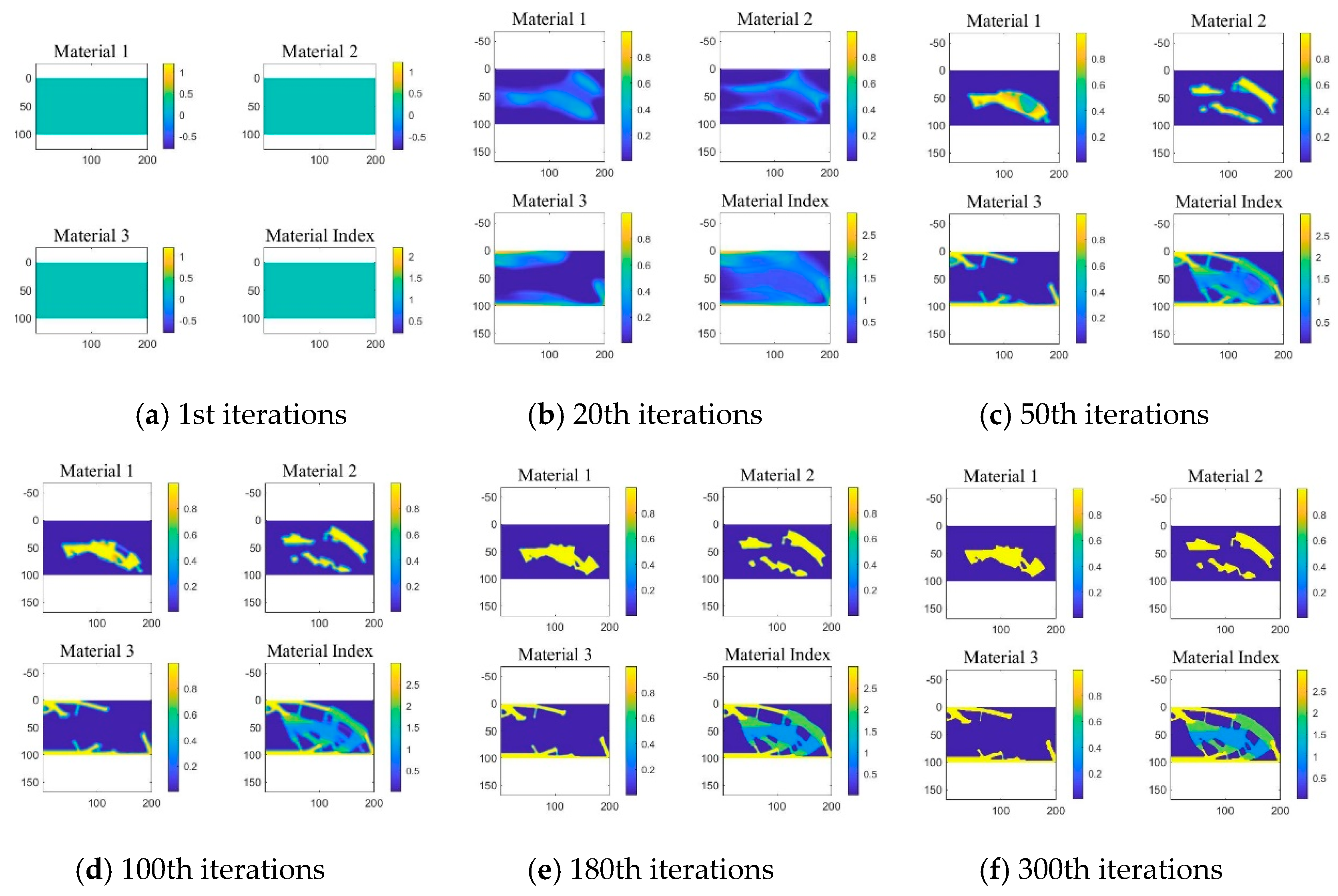
To demonstrate the usability of the code, Figure 1 shows the final design result as well as the iteration details by calling the code in Appendix A. It can be found that the algorithm can converge stably and quickly to a clear result.

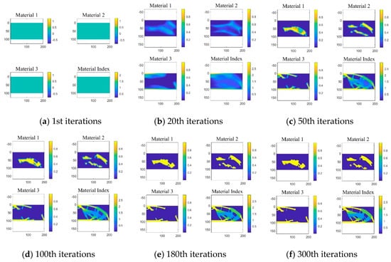
Figure 1. The iteration details of the half MBB beam with three materials.

To obtain the results of these intermediate optimization procedures, the code in Box 4 should be inserted after line 132 of the code in Appendix A. The code divides the figure into four sections, with the first three sections showing the density distributions for each of the three materials and the last section showing the results of the current optimized layout of multi-materials.

Box 4. Current image Display code.

%% PLOT CURRENT DENSIGN

figure(1);

subplot(2,2,1); imagesc(post_x(:,:,1)); axis equal; colorbar; hold on; title(‘Material 1’)

subplot(2,2,2); imagesc(post_x(:,:,2)); axis equal; colorbar; hold on;title(‘Material 2’)

subplot(2,2,3); imagesc(post_x(:,:,3)); axis equal; colorbar;hold on;title(‘Material 3’)

subplot(2,2,4); xx=post_x(:,:,1);

for i=2:NMaterial

xx=xx+i*post_x(:,:,i);

end

imagesc(2.5); imagesc(xx); axis equal; colorbar; hold on; title(‘Material Index’)

4. Numerical Examples

Several numerical examples of the minimum compliance problem are used to illustrate the running results of the Matlab code. The parameters of the above method will affect the final solution similar to conventional methods for topology optimization of continuum structure, and the effect of the parameters is also discussed in this section. The following cases are conducted by using Matlab R2018a on a desktop computer with an Intel CPU 2.8 GHz and 8.0 GB of RAM (Manufacturer: HP, Beijing, China).

4.1. Example 1: The Number of Materials

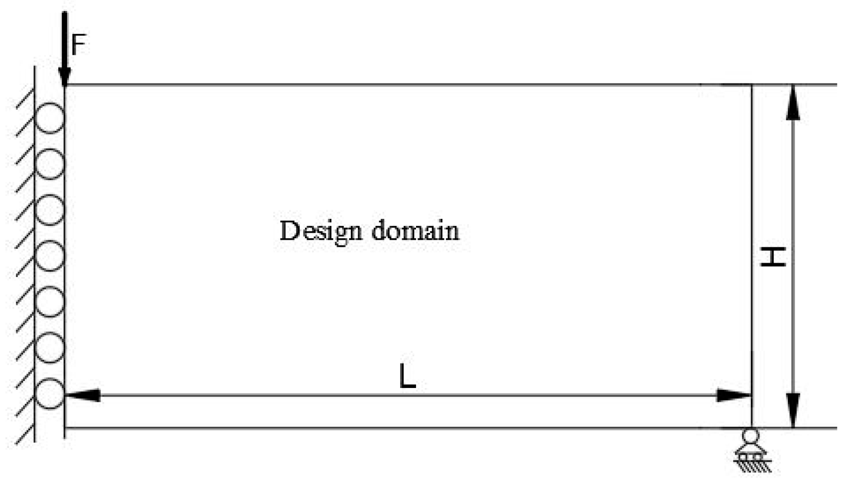
The half MMB beam is taken as an example for the topology optimization of a continuum structure with two, three, and five materials, respectively. The design domain and boundary conditions of the half MBB beam are shown in Figure 2. A load F = −1 is applied at the left upper side of the design domain, and it is simply supported at the bottom corners. The design domain is discretized with 200 × 100 regular elements with Poisson’s ratio µ = 0.3. The initial density of each material is set to 0.5.

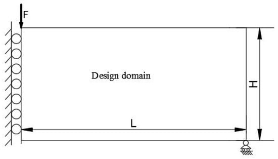
Figure 2. The design domain and boundary conditions of the half MBB beam.

The maximum number of iterations is set as NumIter = 300, the penalty factor is set as penal = 3, the filter radius is set as rmin = 5, and the P-norm parameter p is set as p = 6. The parameter for the projection function starts with beta = 1 and doubles its value after 50 iterations. The volume constraints of two, three, and five materials are set to 0.5/2, 0.5/3, and 0.5/5 for each material, respectively. The Young’s modulus of each material for the three cases is set as follows:

Case 1: two materials par.E(1) = 1; par.E(2) = 5;

Case 2: three materials par.E(1) = 1; par.E(2) = 2; par.E(3) = 5;

Case 3: five materials par.E(1) = 1; par.E(2) = 2; par.E(3) = 3; par.E(4) = 4; par.E(5) = 5;

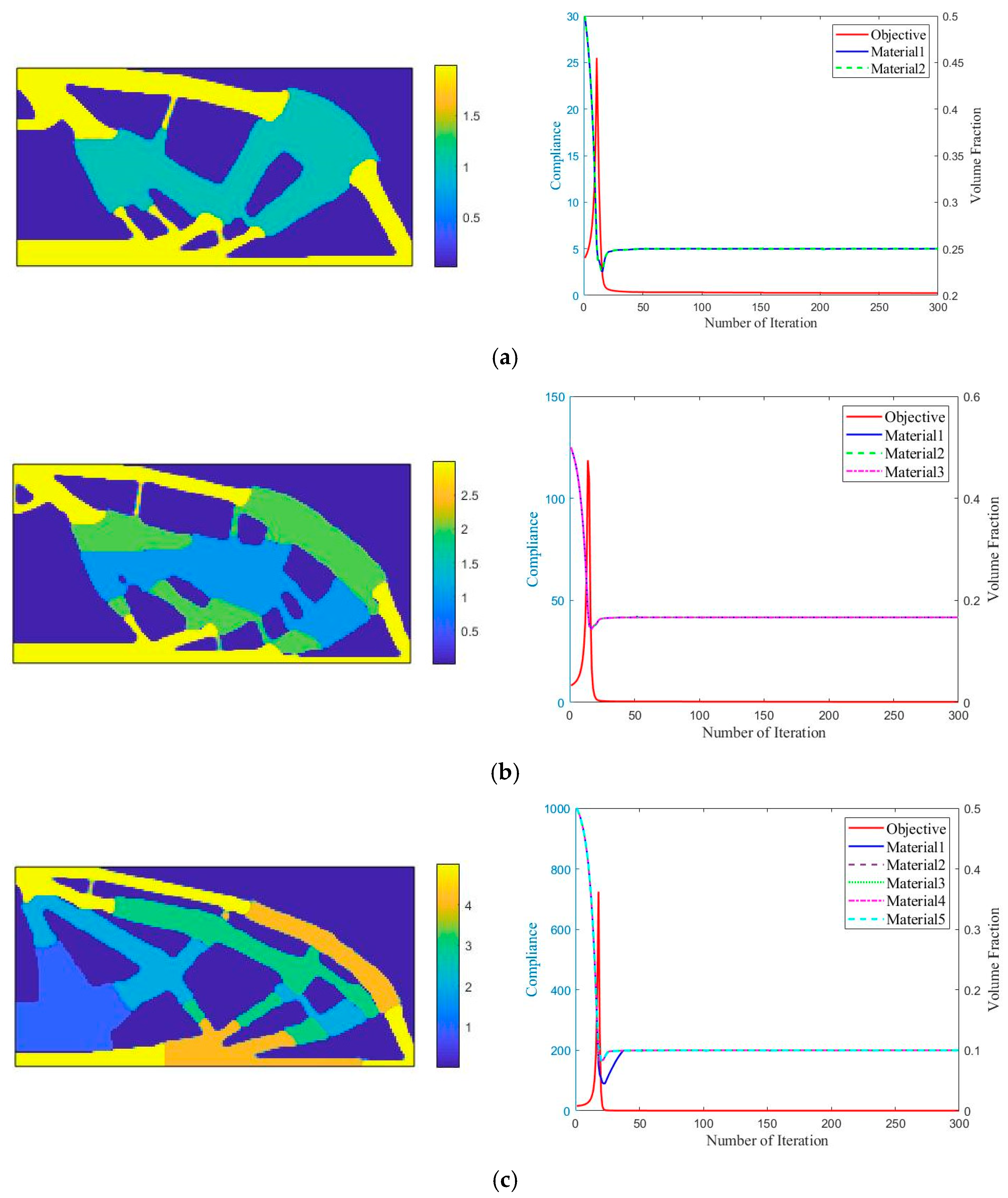
Figure 3 shows the optimized structure and the converged history for topology optimization of different numbers of materials. It can be seen that the code can effectively realize the topology optimization design of multiple materials and obtain clear boundaries for each material. It can be found that the convergence history of the compliance varies little with the number of materials used for optimization, and they converge rapidly in the first 50 iterations. The material volumes also converge rapidly with about 10 iterations. The compliances of the optimized structures for all the cases are almost comparable, and the one with five materials is better than the others, which means that the appropriate layout of multiple materials can improve the stiffness of the optimized structure.

Figure 3. The optimized structure and converge history for topology optimization of different numbers of materials. (a) For two materials, the compliance is 0.249, where cyan and yellow are the materials with E = 1 and E = 5, respectively. (b) For three materials, the compliance is 0.268, where blue, green, and yellow are the materials with E = 1, E = 2, and E = 5, respectively. (c) For five materials, the compliance is 0.242, where blue, cyan, green, orange, and yellow are the materials with E = 1, E = 2, E = 3, E = 4, and E = 5, respectively.

4.2. Example 2: Different Values of Parameter p for the P-Norm

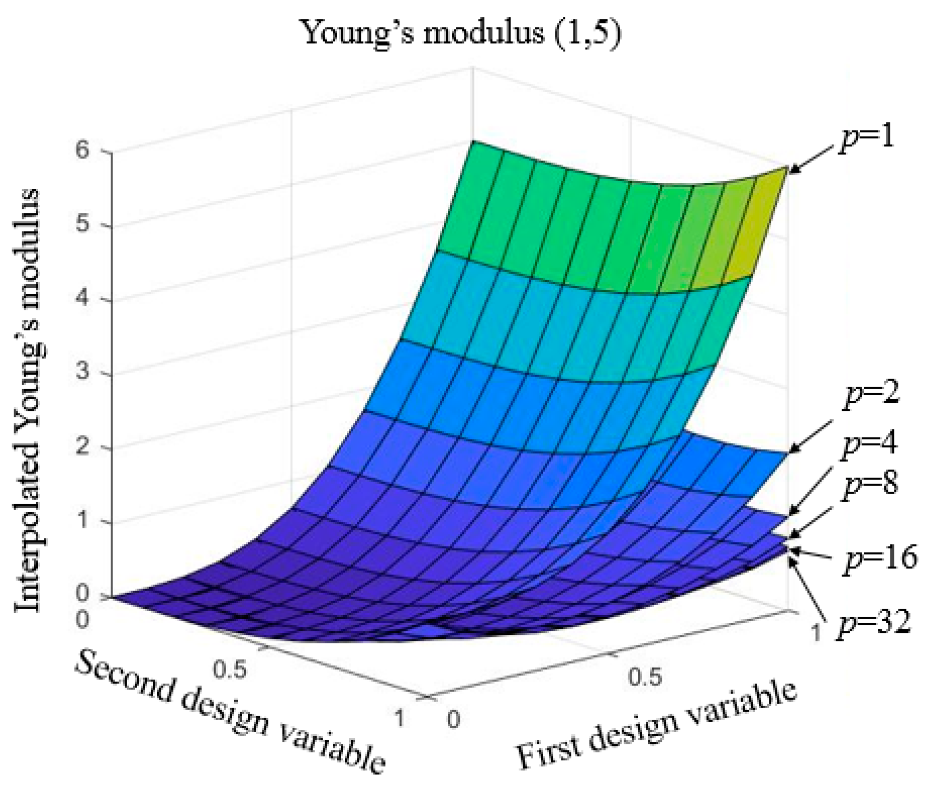
In order to show the influence of the parameter p on the interpolation function of Young’s modulus, a diagram of the interpolated Young’s modulus $\mathrm{E}\left({\overline{\tilde{x}}}_1^e,{\overline{\tilde{x}}}_2^e,\cdots ,{\overline{\tilde{x}}}_{NM}^e\right)$ as a function of parameter p is shown in Figure 4. Here it is assumed that NM = $2$. The Young’s modulus of each material is set as $E_1=1,E_2=5$, with penalty factor n = 3. It can be found that it cannot work well when parameter p is small. As parameter p increases, the interpolated Young’s modulus decreases rapidly at the correct part with both design variables equal to 1. Hence, it will drive the optimization model convergence to a clear result of material 1 and material 2 to be voids or solids.

Figure 4. The function diagram of interpolated Young’s modulus with respect to parameter p.

To further explore the effect of parameter p on the optimization results, the topology optimization of three materials with the half MMB beam using different P-norm values is also studied. The values of parameter p are set as follows:

Case 1: p = 1;

Case 2: p = 6;

Case 3: p = 18;

Case 4: p = 32;

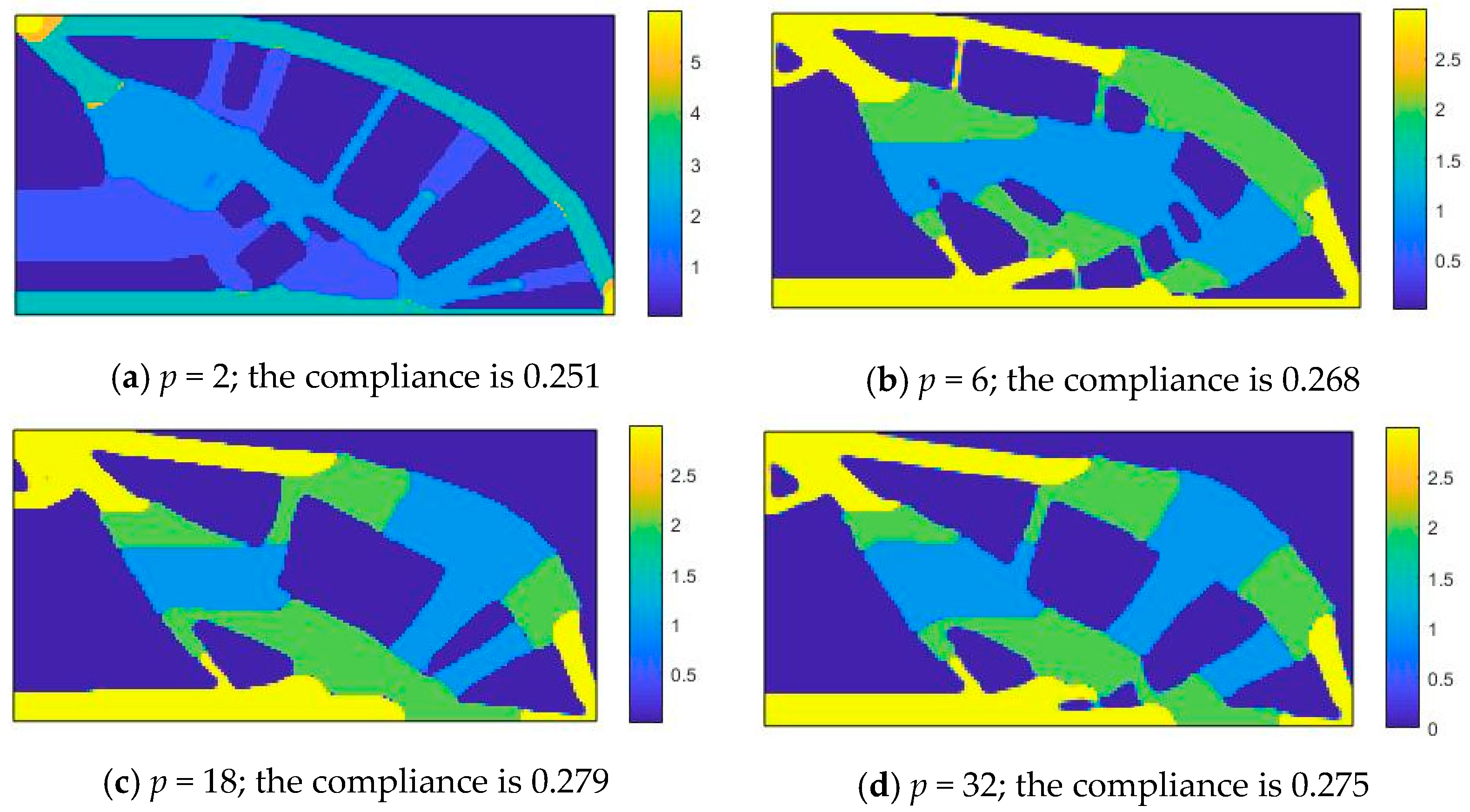
The Young’s modulus of each material is set as par.E(1) = 1; par.E(2) = 2; par.E(3) = 5. The volume constraint is set to 0.5/3 for each material, and other parameters are the same as those in Section 4.1. The optimized structures are shown in Figure 5. It can be found that there are mixed materials at the boundary of the optimized structure when p = 1 because that p-norm function cannot approximate the maximum of the design variable of Equation (4). By increasing the value of parameter p, the boundary of each material becomes clear for the optimized structure, and the compliance of the optimized structures is comparable. However, it will influence the stability of the optimizer with a very large value of parameter p. Therefore, we choose p = 6 in the following examples to balance the structural stiffness and the stability of the optimizer [29].

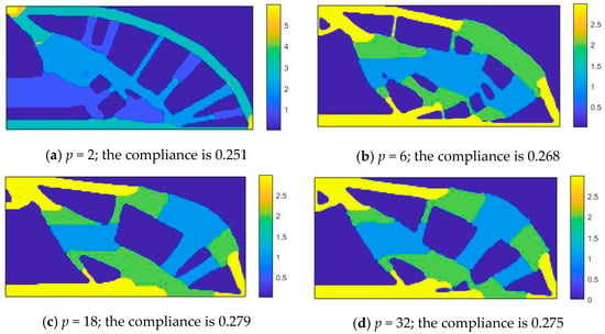
Figure 5. The optimized structure with different values of parameter p for topology optimization of three materials, where blue, green, and yellow are the materials with E = 1, E = 2, and E = 5, respectively.

5. Extension to 3D

The Matlab implementation described in Section 3 is remarkably easy to extend to 3D problems, which can be found in Appendix B.

5.1. 3D Matlab Implementation

The 3D Matlab implementation is verified using a cantilever beam example here. The boundary conditions and loading conditions for the cantilever beam are shown in Figure 4, and the corresponding Matlab code is defined in lines 11–24. A notable modification compared to the 2D Matlab code is the change in the discrete unit element from four-node rectangle elements to eight-node cubic elements. The element stiffness matrix lk is organized in lines 25–40, and the matrix edofMate containing the node IDs for each element is obtained in lines 41–44. The iterative details for the three-material cantilever beam can be obtained by calling the code in lines 157–163. The final design is displayed based on the code top3d.m proposed by Liu [20] in lines 164–200, and the optimized structures with multiple materials are shown in different colors.

5.2. 3D Numerical Examples

5.2.1. Example 1: The Number of Materials

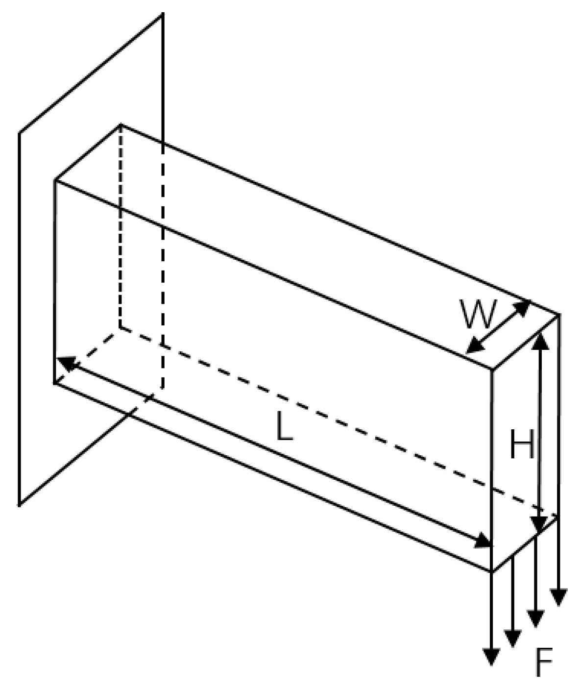
The cantilever beam is taken as an example for the topology optimization of a 3D continuum structure with two, three, and five materials, respectively. The design domain and boundary conditions of the 3D cantilever beam are shown in Figure 6. The left part of the design domain is fixed, and a distributed load F = −1 is applied at the lower right edge. The design domain is discretized into 80 × 40 × 20 cubic elements with Poisson’s ratio µ = 0.3. The initial density of each material is set to 0.5. All other parameters are the same as those in Section 4.1.

Figure 6. The design domain and boundary conditions of the 3D cantilever beam.

The optimized structure and the converged history for topology optimization of different numbers of materials are shown in Figure 7. It can be found that the convergence histories of the compliance are very similar under different numbers of materials, and they converge rapidly in the first 50 iterations, which is similar to the 2D structures. The compliances of the optimized structure with two materials and the optimized structure with three materials are almost comparable, and the structure with five materials has a smaller compliance value. This is a strong demonstration of the advantages of multiple materials in increasing the stiffness of optimized structures from a three-dimensional perspective.

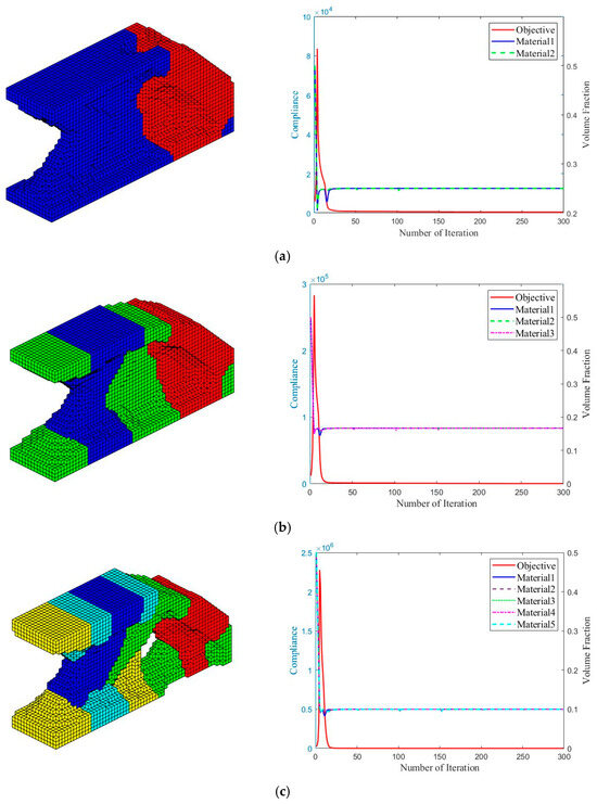
Figure 7. The optimized structure and converge history for topology optimization of multi-materials with 3D cantilever beam. (a) For two materials, the compliance is 432.94, where red and blue are materials with E = 1 and E = 5, respectively. (b) For three materials, the compliance is 433.05, where red, blue, and green are materials with E = 1, E = 2, and E = 5, respectively. (c) For five materials, the compliance is 400.24, where red, blue, cyan, yellow, and green are materials with E = 1, E = 2, E = 3, E = 4, and E = 5, respectively.

5.2.2. Example 2: Different Filter Radii

The topology optimization of the cantilever beam with three materials is taken to test the performance of the code by considering different filter radii to further illustrate the performance of the 3D Matlab code. The filter radii are set as follows:

Case 1: rmin = 2

Case 2: rmin = 5

Case 3: rmin = 8

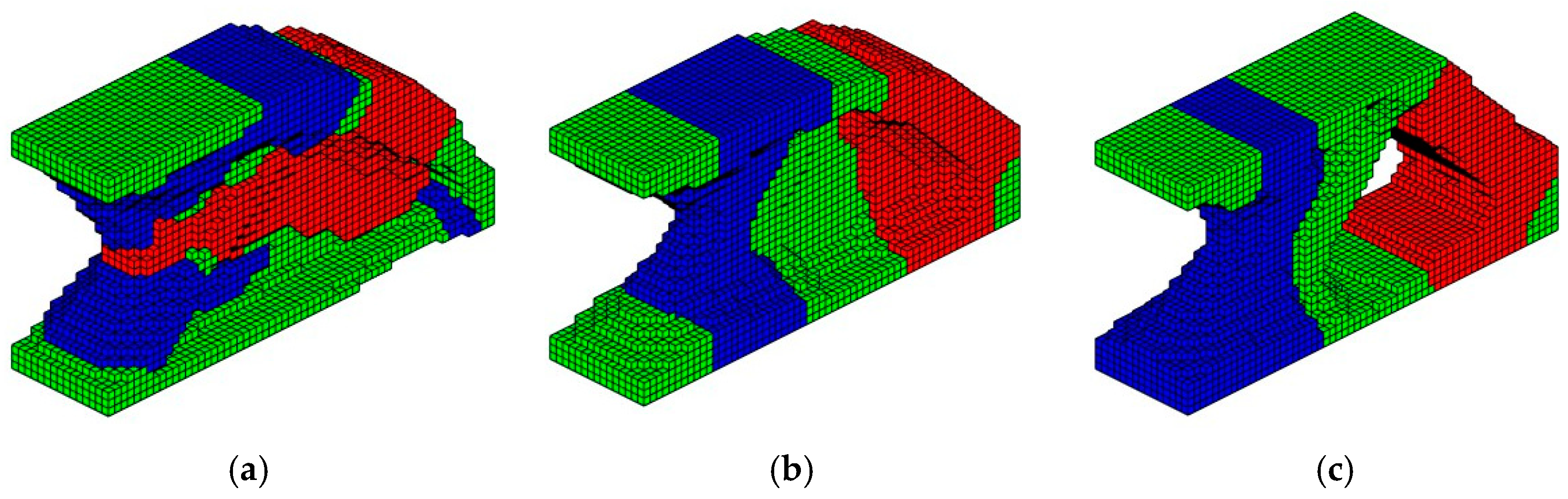
The Young’s moduli are set as par.E(1) = 1; par.E(2) = 2; par.E(3) = 5. The volume constraint is set to 0.5/3 for each material. Other parameters are the same as those in Section 5.2.1. The optimized structures are shown in Figure 8. The results show that the code performs well for feature size control of the optimized structure for topology optimization. Similarly, the topology and the objective function of the optimized structures are changed at different filter radii. As the filter radius is reduced, the advantage of multi-materials is fully utilized with smaller compliance values so that small features can be constructed to get a better local minimum.

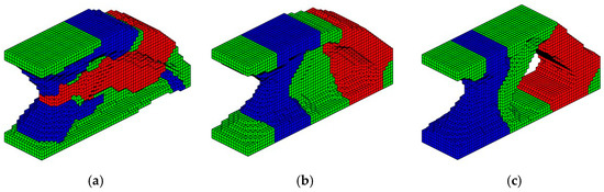
Figure 8. The optimized structure with different filter radii, where red, blue, and green are materials with E = 1, E = 2, and E = 5, respectively. (a) For rmin = 2, the compliance is 382.46. (b) For rmin = 5, the compliance is 433.05. (c) For rmin = 8, the compliance is 539.28.

6. Conclusions

In this paper, simple and efficient 2D and 3D Matlab codes are proposed simultaneously to reduce the barrier of the implementation of multi-material topology optimization. Multi-material topology optimization with the map-based interpolation function proposed by Yi [16] et al. is implemented. The density filter is used to resolve the issues of mesh-dependent and checker-board problems. The projection function is used to ensure a 0–1 solution. The MMA algorithm is used to solve the minimum compliance problem under volume constraints. The algorithm is an extension of the 88-line code for the SIMP-based topology optimization of single materials, and we hope it can provide an educational instrument for newcomers to the field of multi-material topology optimization. Numerical examples of 2D structures with different materials and P-norm parameter p and 3D structures with different materials and filter radii are given to prove the effectiveness of the code.

References

- Huang, X.; Li, W. A new multi-material topology optimization algorithm and selection of candidate materials. Comput. Methods Appl. Mech. Eng. 2021, 386, 114114. [Google Scholar] [CrossRef]
- Liu, W.; Yoon, G.H.; Yi, B.; Choi, H.; Yang, Y. Controlling wave propagation in one-dimensional structures through topology optimization. Comput. Struct. 2020, 241, 106368. [Google Scholar] [CrossRef]
- Yang, X.; Li, M. Discrete multi-material topology optimization under total mass constraint. Comput.-Aided Des. 2018, 102, 182–192. [Google Scholar] [CrossRef]
- Bohrer, R.; Kim, I.Y. Multi-material topology optimization considering isotropic and anisotropic materials combination. Struct. Multidisc. Optim. 2021, 64, 1567–1583. [Google Scholar] [CrossRef]
- Liu, B.; Huang, X.; Cui, Y. Topology optimization of multi-material structures with explicitly graded interfaces. Comput. Methods Appl. Mech. Eng. 2022, 398, 115166. [Google Scholar] [CrossRef]
- Chandrasekhar, A.; Suresh, K. Multi-Material Topology Optimization Using Neural Networks. Comput.-Aided Des. 2021, 136, 103017. [Google Scholar] [CrossRef]
- Zhang, X.S.; Paulino, G.H.; Ramos, A.S. Multi-material topology optimization with multiple volume constraints: A general approach applied to ground structures with material nonlinearity. Struct. Multidisc. Optim. 2018, 57, 161–182. [Google Scholar] [CrossRef]
- Shah, V.; Pamwar, M.; Sangha, B.; Kim, I.Y. Multi-material topology optimization considering natural frequency constraint. Eng. Comput. 2022, 39, 2604–2629. [Google Scholar] [CrossRef]
- Sigmund, O.; Torquato, S. Design of materials with extreme thermal expansion using a three-phase topology optimization method. J. Mech. Phys. Solids 1997, 45, 1037–1067. [Google Scholar] [CrossRef]
- Hvejsel, C.F.; Lund, E. Material interpolation schemes for unified topology and multi-material optimization. Struct. Multidisc. Optim. 2011, 43, 811–825. [Google Scholar] [CrossRef]
- Stegmann, J.; Lund, E. Discrete material optimization of general composite shell structures. Int. J. Numer. Meth. Eng. 2005, 62, 2009–2027. [Google Scholar] [CrossRef]
- Gao, T.; Zhang, W. A mass constraint formulation for structural topology optimization with multiphase materials. Int. J. Numer. Meth. Eng. 2011, 88, 774–796. [Google Scholar] [CrossRef]
- Bruyneel, M. SFP—A new parameterization based on shape functions for optimal material selection: Application to conventional composite plies. Struct. Multidisc. Optim. 2011, 43, 17–27. [Google Scholar] [CrossRef]
- Yin, L.; Ananthasuresh, G.K. Topology optimization of compliant mechanisms with multiple materials using a peak function material interpolation scheme. Struct. Multidiscip. Optim. 2001, 23, 49–62. [Google Scholar] [CrossRef]
- Zuo, W.; Saitou, K. Multi-material topology optimization using ordered SIMP interpolation. Struct. Multidiscip. Optim. 2017, 55, 477–491. [Google Scholar] [CrossRef]
- Yi, B.; Yoon, G.H.; Zheng, R.; Liu, L.; Li, D.; Peng, X. A unified material interpolation for topology optimization of multi-materials. Comput. Struct. 2023, 282, 107041. [Google Scholar] [CrossRef]
- Bendsøe, M.P.; Kikuchi, N. Generating optimal topologies in structural design using a homogenization method. Comput. Methods Appl. Mech. Eng. 1988, 71, 197–224. [Google Scholar] [CrossRef]
- Sigmund, O. A 99 line topology optimization code written in Matlab. Struct. Multidisc. Optim. 2001, 21, 120–127. [Google Scholar] [CrossRef]
- Andreassen, E.; Clausen, A.; Schevenels, M.; Lazarov, B.S.; Sigmund, O. Efficient topology optimization in MATLAB using 88 lines of code. Struct. Multidisc. Optim. 2011, 43, 1–16. [Google Scholar] [CrossRef]
- Liu, K.; Tovar, A. An efficient 3D topology optimization code written in Matlab. Struct. Multidiscip. Optim. 2014, 50, 1175–1196. [Google Scholar] [CrossRef]
- Ferrari, F.; Sigmund, O. A new generation 99 line Matlab code for compliance topology optimization and its extension to 3D. Struct. Multidiscip. Optim. 2020, 62, 2211–2228. [Google Scholar] [CrossRef]
- Huang, X.; Xie, Y.-M. A further review of ESO type methods for topology optimization. Struct. Multidiscip. Optim. 2010, 41, 671–683. [Google Scholar] [CrossRef]
- Challis, V.J. A discrete level-set topology optimization code written in Matlab. Struct. Multidiscip. Optim. 2010, 41, 453–464. [Google Scholar] [CrossRef]
- Wei, P.; Li, Z.; Li, X.; Wang, M.Y. An 88-line MATLAB code for the parameterized level set method based topology optimization using radial basis functions. Struct. Multidiscip. Optim. 2018, 58, 831–849. [Google Scholar] [CrossRef]
- Zhang, W.; Yuan, J.; Zhang, J.; Guo, X. A new topology optimization approach based on Moving Morphable Components (MMC) and the ersatz material model. Struct. Multidiscip. Optim. 2016, 53, 1243–1260. [Google Scholar] [CrossRef]
- Du, Z.; Cui, T.; Liu, C.; Zhang, W.; Guo, Y.; Guo, X. An efficient and easy-to-extend Matlab code of the Moving Morphable Component (MMC) method for three-dimensional topology optimization. Struct. Multidiscip. Optim. 2022, 65, 158. [Google Scholar] [CrossRef]
- Xia, L.; Breitkopf, P. Design of materials using topology optimization and energy-based homogenization approach in Matlab. Struct. Multidiscip. Optim. 2015, 52, 1229–1241. [Google Scholar] [CrossRef]
- Dong, G.; Tang, Y.; Zhao, Y.F. A 149 Line Homogenization Code for Three-Dimensional Cellular Materials Written in matlab. J. Eng. Mater. Technol. 2019, 141, 011005. [Google Scholar] [CrossRef]
- Liu, P.; Yan, Y.; Zhang, X.; Luo, Y. A MATLAB code for the material-field series-expansion topology optimization method. Front. Mech. Eng. 2021, 16, 607–622. [Google Scholar] [CrossRef]
- Tavakoli, R.; Mohseni, S.M. Alternating active-phase algorithm for multimaterial topology optimization problems: A 115-line MATLAB implementation. Struct. Multidiscip. Optim. 2014, 49, 621–642. [Google Scholar] [CrossRef]
- Sanders, E.D.; Pereira, A.; Aguiló, M.A.; Paulino, G.H. PolyMat: An efficient Matlab code for multi-material topology optimization. Struct. Multidiscip. Optim. 2018, 58, 2727–2759. [Google Scholar] [CrossRef]
- Gangl, P. A multi-material topology optimization algorithm based on the topological derivative. Comput. Methods Appl. Mech. Eng. 2020, 366, 113090. [Google Scholar] [CrossRef]
- Wang, F.; Lazarov, B.S.; Sigmund, O. On projection methods, convergence and robust formulations in topology optimization. Struct. Multidiscip. Optim. 2011, 43, 767–784. [Google Scholar] [CrossRef]
- Xu, S.; Cai, Y.; Cheng, G. Volume preserving nonlinear density filter based on heaviside functions. Struct. Multidiscip. Optim. 2010, 41, 495–505. [Google Scholar] [CrossRef]
- Svanberg, K. The method of moving asymptotes—A new method for structural optimization. Numer. Meth. Eng. 1987, 24, 359–373. [Google Scholar] [CrossRef]
Disclaimer/Publisher’s Note: The statements, opinions and data contained in all publications are solely those of the individual author(s) and contributor(s) and not of MDPI and/or the editor(s). MDPI and/or the editor(s) disclaim responsibility for any injury to people or property resulting from any ideas, methods, instructions or products referred to in the content. |
© 2024 by the authors. Licensee MDPI, Basel, Switzerland. This article is an open access article distributed under the terms and conditions of the Creative Commons Attribution (CC BY) license (https://creativecommons.org/licenses/by/4.0/).