Abstract
Marine heatwaves (MHWs) refer to a phenomenon where the sea surface temperature is significantly higher than the historical average for that region over a period, which is typically a result of the combined effects of climate change and local meteorological conditions, thereby potentially leading to alterations in marine ecosystems and an increased incidence of extreme weather events. MHWs have significant impacts on the marine environment, ecosystems, and economic livelihoods. In recent years, global warming has intensified MHWs, and research on MHWs has rapidly developed into an important research frontier. With the development of deep learning models, they have demonstrated remarkable performance in predicting sea surface temperature, which is instrumental in identifying and anticipating marine heatwaves (MHWs). However, the complexity of deep learning models makes it difficult for users to understand how the models make predictions, posing a challenge for scientists and decision-makers who rely on interpretable results to manage the risks associated with MHWs. In this study, we propose an interpretable model for discovering MHWs. We first input variables that are relevant to the occurrence of MHWs into an LSTM model and use a posteriori explanation method called Expected Gradients to represent the degree to which different variables affect the prediction results. Additionally, we decompose the LSTM model to examine the information flow within the model. Our method can be used to understand which features the deep learning model focuses on and how these features affect the model’s predictions. From the experimental results, this study provides a new perspective for understanding the causes of MHWs and demonstrates the prospect of future artificial intelligence-assisted scientific discovery.
1. Introduction
Since the beginning of the 21st century, there has been particular attention to extreme weather and hydrological and oceanic events such as heatwaves, cold waves, storms, floods, and tropical cyclones, which often lead to complex consequences and, in some cases, catastrophic outcomes [1]. Marine heatwaves (MHWs) [2] are extreme heat events that occur in the ocean, resulting from the combined influence of atmospheric and oceanic processes. They can persist for several days to several months and can span from a few square kilometers to thousands of square kilometers. MHWs have significant destructive impacts on marine environments, marine ecosystems, and socioeconomic development. Studies have shown that MHWs can cause widespread coral bleaching and reductions in kelp forests and seagrass meadows, thereby compromising marine biodiversity, fisheries, and aquaculture [3,4,5]. With the warming of the ocean and climate [6], significant changes have been observed, from large-scale ocean circulation [7,8,9] to mesoscale ocean processes [10,11]. Therefore, accurately predicting marine heatwaves has become a current research focus.
MHWs are identified by SSTs that are unusually high for an extended period, typically exceeding a predefined threshold such as the 90th percentile of historical SST data for a given area [12]. Therefore, SST prediction is the key to anticipating and mitigating the impacts of these extreme events. In the field of marine science, deep learning has shown remarkable potential, providing new perspectives and tools for understanding and addressing ocean-related issues [13]. Compared to statistical methods, deep learning can establish nonlinear mapping relationships between oceanic variables and other features more conveniently, with adaptability and higher predictive accuracy. In recent years, the application of deep learning in marine heatwave prediction has become a research hotspot. Zhang et al. [14] proposed the use of LSTM models to address sea surface temperature (SST) prediction, demonstrating the effectiveness of this method with small prediction errors. Ham et al. [15] applied a CNN model to ENSO prediction, demonstrating that the CNN model is an advanced approach for analyzing the complex mechanisms of ENSO events. In 2021, an all-season CNN model was created, incorporating seasonality in climate data [16]. Prasad et al. [17] used random forests and the N-BEATS model to predict sea surface temperature at the seasonal scale, and then used the predicted SST data to forecast the occurrence of marine heatwaves one year in advance.These studies have demonstrated that deep learning models hold scientific significance in predicting marine heatwaves.
Currently, existing deep learning prediction models are entirely data-driven. The non-linear elements implemented inside the model use activation functions like Sigmoid, tanh, etc., which exhibit strong non-convexity. Internally, the network can be regarded as a “black box”, lacking interpretability in dimensions such as time and space [18]. In recent years, the research on the interpretability of deep learning has attracted widespread attention. Scholars around the world have overviewed the field of explainable artificial intelligence from different research angles and emphases [19]. Although there is a lack of specific mathematics and a universally accepted definition of interpretability, this term typically pertains to the causal relationship between inputs and outputs [20]. Guidotti et al. [21] provides a comprehensive review and detailed categorization of methods for explaining machine learning models, including various deep learning networks. Some new interpretability methods have been developed to explain the predictive patterns captured by the machine within the recurrent units of LSTM networks [22,23,24]. Most interpretability methods were initially designed for symbolic sequences in natural language processing, which is different from analyzing the relationships between oceanic variables with specific physical meaning and real-world context. Explainable artificial intelligence aims to build more understandable models while maintaining a high level of performance, making the decisions of deep neural network models more transparent, interpretable, and trustworthy for humans. However, few studies have explored the underlying principles behind LSTM network decisions, especially regarding the exact role of the well-known memory mechanism in predicting oceanic variables. Therefore, new methods are needed to address the heterogeneity of the data in multidimensional-level prediction and make these predictions interpretable.
In this article, inspired by Jiang et al. [25], we introduce a novel interpretable artificial intelligence approach that focuses on the identification of marine heatwave patterns. Particularly, understanding the causes of marine heatwave generation in the context of climate change helps in identifying and mitigating the risks of flood disasters. We establish an LSTM-based model, selecting 13 coastal stations in China. Using two advanced interpretability techniques, namely Expected Gradients and Additive Decomposition, we analyze the variations of information hidden within the network to reveal the role of the model in identifying marine heatwaves.
2. Methods
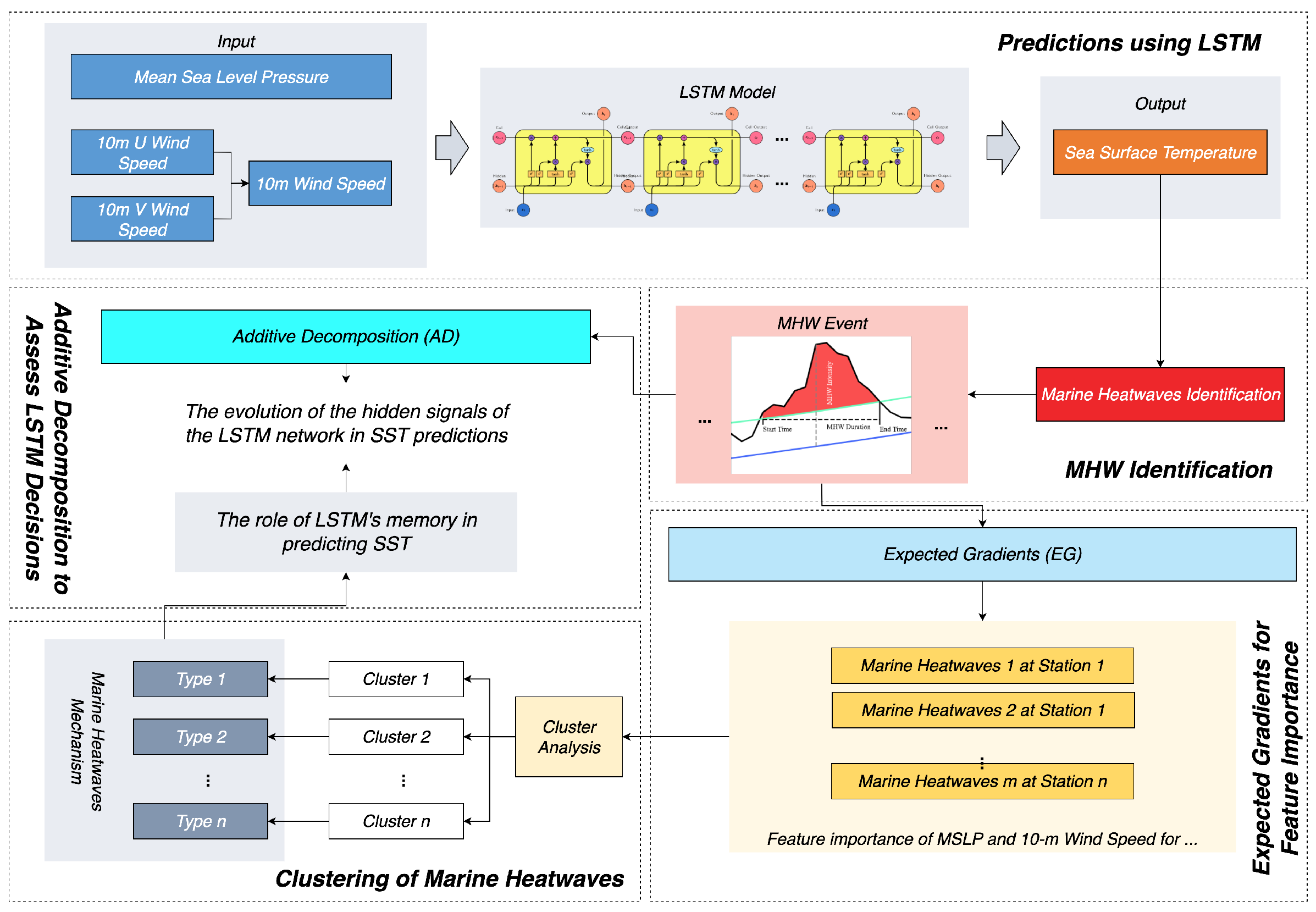
In this paper, we present the framework of predicting marine heatwaves, as depicted in Figure 1. We establish a nonlinear predictive relationship between oceanic meteorological factors and sea surface temperature (SST) using an LSTM model. The temporal importance of meteorological input variables is explained using the Expected Gradients (EG) method. Then, the types of heatwave events are revealed through cluster analysis. Additionally, we investigate the memory mechanism of the LSTM network in simulating different types of heatwave events using the Additive Decomposition (AD) method. The specific workflow is as follows:

Figure 1.
The framework of using interpretive deep learning for marine heatwaves.
We first utilize the LSTM model to establish a nonlinear predictive relationship between oceanic meteorological factors and SST within the target marine heatwave region. To predict the occurrence of heatwave events, we select daily sea surface temperature, sea surface pressure, 10m zonal wind speed, and 10m meridional wind speed as input variables, as they are closely related to the formation and development of marine heatwaves.
To explain the temporal importance of the meteorological input variables (sea surface pressure, 10m zonal wind, and 10m meridional wind) in the model’s prediction of marine heatwaves, we apply a state-of-the-art interpretability technique called Expected Gradients (EG) [26]. By employing the EG method, we obtain importance scores for sea surface pressure, 10m zonal wind, and 10m meridional wind for each target heatwave event.
By interpreting these feature importance scores, we can reveal the mechanisms of heatwave events. For this purpose, cluster analysis is employed in this study to group the predictive results of marine heatwave events based on similar patterns of feature importance, with different clusters potentially associated with different heatwave event mechanisms.
To investigate the different behaviors of the LSTM network’s memory mechanism in simulating different types of heatwave events, we employ another interpretability technique called Additive Decomposition (AD) [27]. In contrast to the EG method, the focus of the AD method is to study the detailed evolution of signals within the hidden units of the LSTM network that influence predictions.
The experimental setup in this study incorporated the following hardware and environmental configurations. The hardware consisted of a CPU, the Intel Xeon Gold 6130; graphics cards, with two NVIDIA GeForce RTX 2080 Ti, each having 11 GB of video memory; system memory with a capacity of 251 GB DDR4; and 3.6 TB of hard disk storage. The software environment was based on the Ubuntu 16.04 LTS operating system, using Python 3.7.0 as the programming language. Dependency libraries included the deep learning library TensorFlow 1.13.1 and the interpretability toolkit Shap 0.42.1, with CUDA version 11.3 installed. The model prediction evaluation metrics were MSE (Mean Squared Error) and RMSE (Root Mean Squared Error). The operating principles and steps of each module are introduced in the following sections.
2.1. Prediction Using the LSTM Network
2.1.1. Data
Table 1 summarizes the observation and reanalysis datasets used in this study. The OISST V2 dataset provided by the National Oceanic and Atmospheric Administration (NOAA) of the United States is derived from remotely sensed SST by the Advanced Very High-Resolution Radiometer (AVHRR), and estimates global high-resolution daily sea surface temperature using an optimal interpolation (OI) method. The dataset resolution is 0.25° × 0.25°, spanning from 1982 to 2020. ERA5 is the fifth generation of atmospheric reanalysis conducted by the European Centre for Medium-Range Weather Forecasts (ECMWF). ERA5 provides hourly estimates of numerous atmospheric, land, and oceanic variables from 1979 to the present. The variables used in this paper include sea surface pressure (P), 10m zonal wind (U), and 10 m meridional wind (V), with the dataset resolution being 0.25° × 0.25°. The U and V can describe the wind motion state. Based on this, the wind speed and direction can be calculated using vector direction and strength concepts. The wind speed is calculated using the formula , and the wind direction by . The function is a four-quadrant inverse tangent operation, which yields the azimuthal angle from the origin to a point in space. By inputting the components U and V, the wind direction angle can be determined. The output is given in radians with a range of . The obtained angle is measured counterclockwise from true north. If measurement clockwise from true north is desired, it should be converted to .

Table 1.
The Observational and Reanalysis Data Sets Used in This Study.
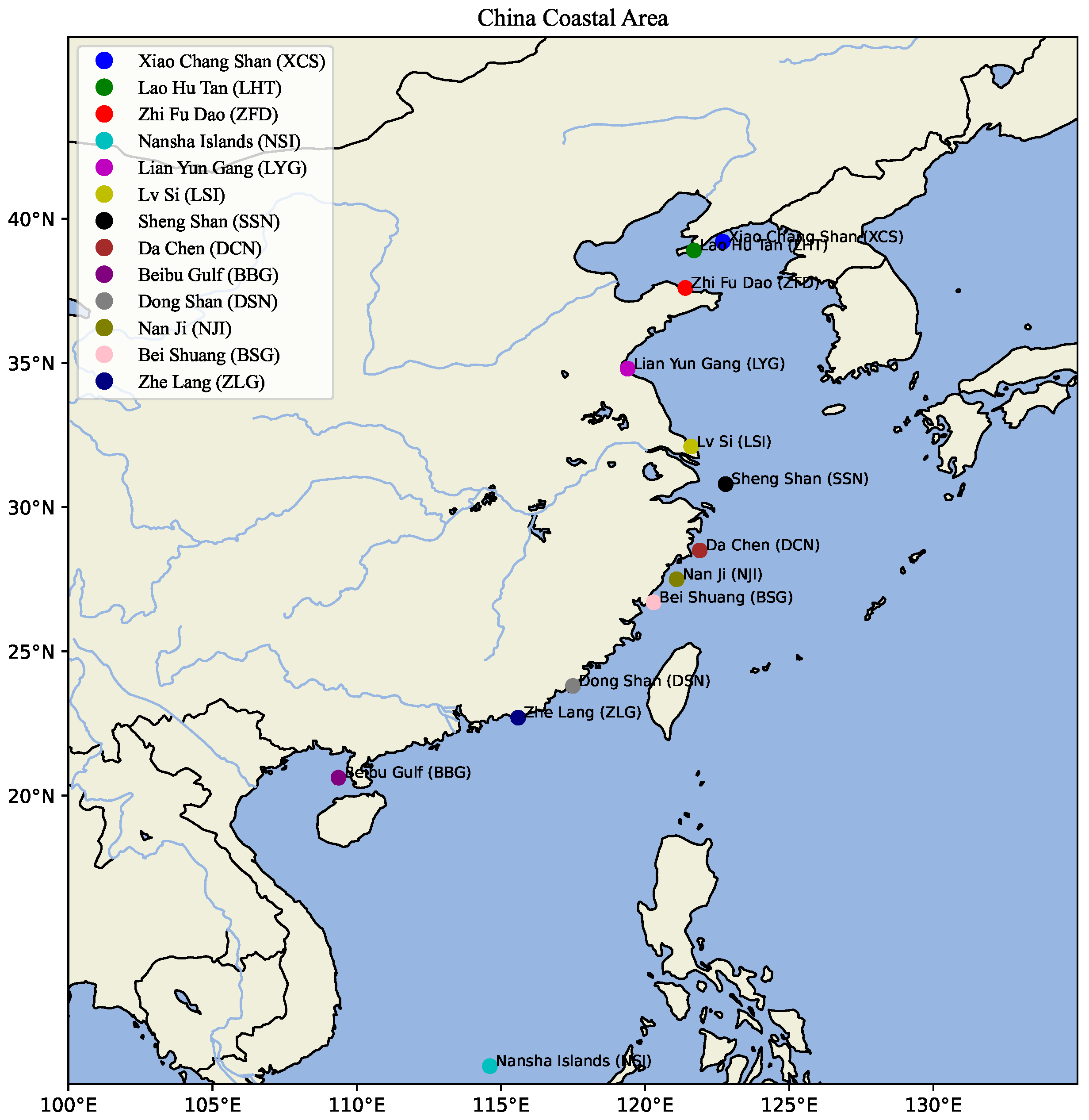
In this study, we chose datasets for different stations along the Chinese coast as our research subjects. The Chinese coastal areas include the East China Sea, South China Sea, and Yellow Sea, among others, with these areas having plenty of marine resources and crucial ecosystems. Our dataset selection is based on the following considerations. 1. The geographical significance of the coastal sites to China’s marine biodiversity hotspots and fishing grounds, which are vital for preserving species diversity and ensuring food security. 2. The sensitivity of these regions to climatic anomalies and anthropogenic impacts, which make them sentinel areas for detecting the early signs of climate change-driven phenomena like marine heatwaves. 3. The potential socio-economic repercussions resulting from changes in the marine ecosystem that could affect coastal communities, including alterations in fisheries, tourism, and local livelihoods. We chose thirteen stations, and Table 2 shows the latitudes and longitudes of these stations, with their positions on the map depicted in Figure 2.
Table 2.
The longitude and latitude information of the various stations taken in the coastal sea areas of China.
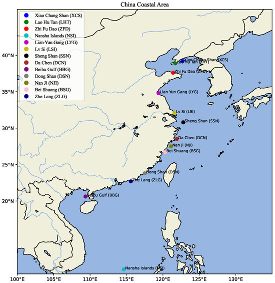
Figure 2.
The locations of the various stations taken in the coastal ocean areas of China.
2.1.2. LSTM Model
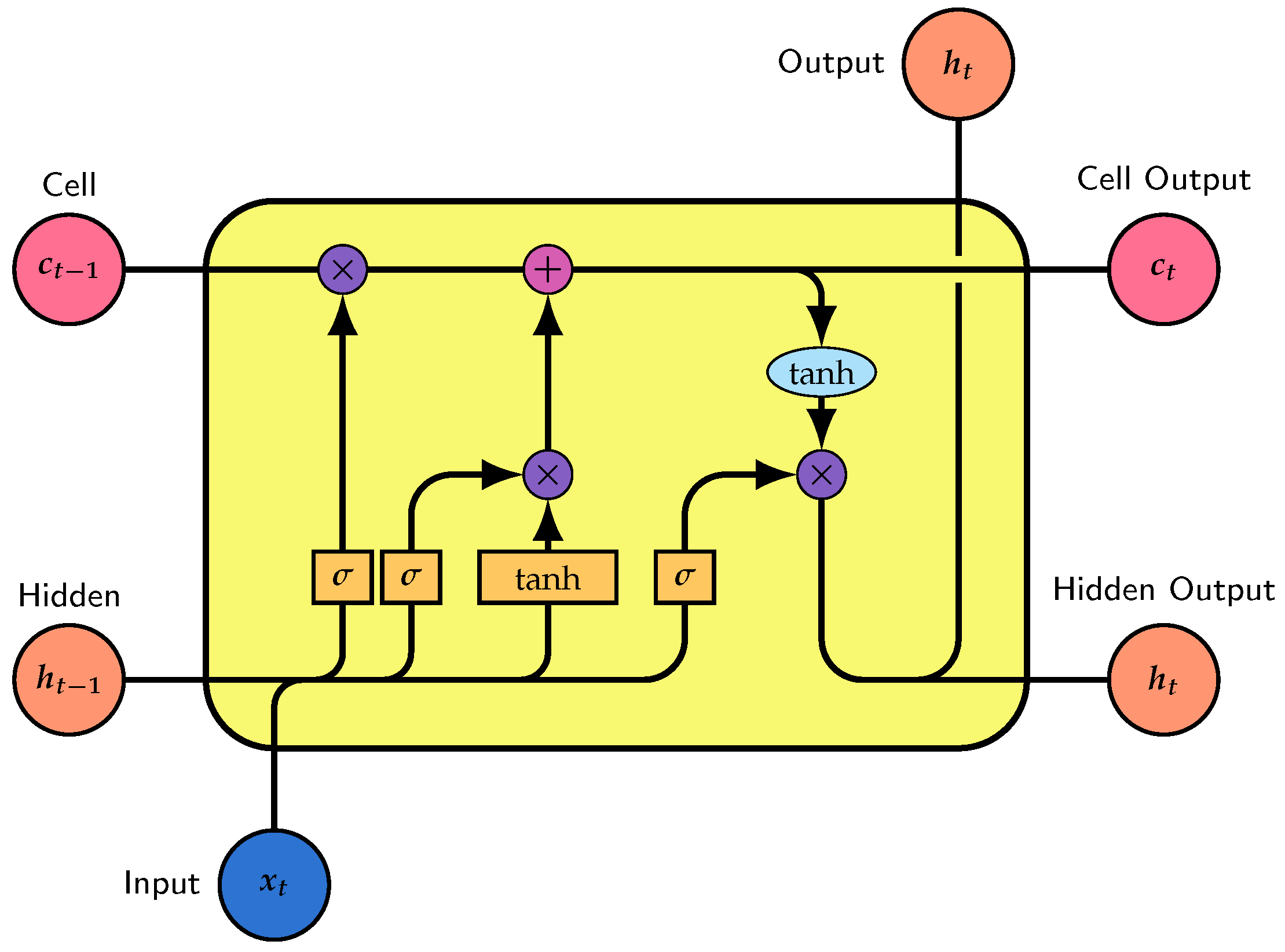
Due to the design of gating mechanisms and memory units, the LSTM model [30] is able to flexibly store, forget, and update information in time series data. This allows LSTM to effectively capture long-term dependencies in time series and demonstrate excellent performance in tasks such as prediction and sequence generation. Additionally, this model aids in decomposing internal signals. In the context of the marine heatwave problem, the model used in this study consists of an LSTM layer and a dense layer to predict sea surface temperature. The SST at each station is treated as time series data. The model takes the daily [P,U,V] of the previous 180 time steps as the input sequence (, ) to predict the sea surface temperature and identify occurrences of marine heatwave events. The LSTM network operates in a chain-like manner, passing information through recurrent units and performing long-term memory and nonlinear transformations through the computation of cell states and hidden states. The LSTM includes a cell state vector that maintains the network’s long-term memory and a hidden state vector that serves as the non-linear transform output of the cell state. At each time step t, the recurrent unit receives the cell state and hidden state from the previous unit ( and ) as well as the current input (), and computes the current cell state and hidden state ( and ) for use by subsequent units. The hidden state of the last time step is then mapped to a single neuron through the dense layer to obtain the prediction result. Figure 3 illustrates the structure of a single LSTM unit.
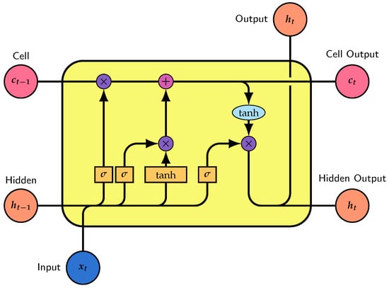
Figure 3.
This is an LSTM cell unit that includes a cell state vector , a hidden state vector , and the current input .
Figure 3 presents the architecture of an LSTM unit, which includes four multilayer perceptrons that are based on the prior hidden state and current input to calculate the forget gate (), candidate cell state (), input gate (), and output gate (). It then linearly updates the cell state (). Using the output gate and the new cell state (), a nonlinear transformation is applied to produce the hidden state ().
The operations of the LSTM can be represented with the following mathematical expressions:
where and are weights and biases that need to be determined during training, and denote the sigmoid function and the hyperbolic tangent function, respectively, and ⊙ signifies element-wise multiplication. Within the model, three gates control the flow of information; amalgamates prior and current information, while considers the input across all time steps. The and of a multi-unit LSTM followed by a fully connected layer are used to reduce dimensionality for predictions. The training process employs the Adaptive Moment Estimation (Adam) algorithm [31] alongside an early stopping strategy to prevent overfitting. The dataset is randomly divided into a training set and a validation set, with 70% of the data used for training and 30% designated for independent evaluation of the model’s performance. By independently training models at each site, the variations in observed MHWs over different periods are captured, thereby enhancing the robustness of the model’s evaluation and analysis.
2.2. Marine Heat Waves (MHWs) Definition and Indices
Marine heatwaves are mutually discrete and persistent anomalous warming events that occur in the ocean. In general, the determination of whether an extremely high SST event is a marine heatwave is based primarily on whether SST exceeds the marine heatwave threshold for multiple consecutive days [32]. Currently, there are two main types of marine heatwave thresholds that are commonly used. One is a fixed SST threshold, called the Absolute Threshold, and the other is a selected threshold that varies over time, named Relative Threshold (or Comparative Threshold). The function in previous studies to find MHW events includes absolute temperature threshold, cumulative threshold, temporally fixed threshold, and high percentile threshold [32,33,34]. The absolute temperature threshold is determined with reference to factors such as environmental elements and the upper absolute temperature to which marine organisms can adapt, while the threshold determined by accumulating the temperature difference above the absolute temperature threshold is called the accumulation threshold [32,33].
For quantitative analysis of marine heatwaves, Hobday et al. [12] provided a stricter definition considering the duration, intensity, rate of evolution, and spatial extent of MHW events. Figure 4 illustrates several MHW events that occurred at the ZLG station (115.625 N, 22.625 E) from March to September 2021, with a zoomed-in area showcasing an MHW event in March–April 2021. From Figure 4, it can be observed that the MHW event began when the sea surface temperature (SST) first exceeded the MHW threshold after 24 March 2021. The SST reached its peak during the middle phase of the event. Subsequently, it fell below the MHW threshold in early April and remained below the threshold, indicating the end of the MHW event. The duration of this event corresponds to the time span it covered, and the difference between the peak SST and the climatological mean SST represents the intensity of the MHW event during that period.
The calculation formula for the climatological mean can be expressed as shown in Table 3. Here, temperature T is expressed as a function of time t, as well as a function of year y and day of the year d. represents the climatological average temperature calculated over a reference period. defines the seasonal threshold temperature value for marine heatwaves (MHWs), and D signifies the duration over which the temperature exceeds this threshold. Within the context of a MHW event, indicates the maximum temperature anomaly, represents the mean temperature anomaly during the MHW, and signifies the variation in MHW intensity over the duration of the event.
Table 3.
Indicators characterizing marine heatwaves (MHWs). In the formula, j represents a specific day within a year, and denote the start and end of the climatological baseline period, respectively, and T is the daily Sea Surface Temperature (SST) for day d of year y. represents the 90th percentile, where pertains to the set . The term denotes the standard deviation, and the time period is defined from to , with the day j falling within the window .
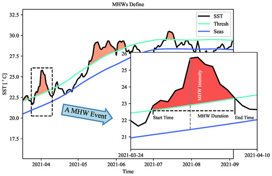
Figure 4.
Several marine heatwave events occurred between March and August 2021 at coordinates (115.625 N, 22.625 E). The marine heatwave events from March to April are used to define marine heatwaves, and the specific definition and formula can be found in Table 4.
Table 4.
Perform four independent experiments at 13 stations, with the Mean Squared Error (MSE) and Root Mean Squared Error (RMSE) results for each experiment.
Figure 4.
Several marine heatwave events occurred between March and August 2021 at coordinates (115.625 N, 22.625 E). The marine heatwave events from March to April are used to define marine heatwaves, and the specific definition and formula can be found in Table 4.

Hobday et al. [12] classified MHWs based on the intensity of MHWs, using the following definition:
MHWs can be categorized into several classes based on the magnitude of N. The term represents the temperature anomaly with as the temperature threshold and as the climatological mean temperature. The intensity of an MHW is denoted by . When , the event is classified as a moderate-intensity event (Category I); when , it is classified as a strong MHW event (Category II); when , the event is considered severe (Category III); and when , the event is classified as extreme (Category IV). After identifying MHW events, the following indices are used to describe the characteristics of MHWs: the number of MHW events () N, the total number of MHW days (), and the average duration of MHWs ().
2.3. Expected Gradients for Feature Importance
To enhance the interpretability of decision-making by data-driven models, the Expected Gradients (EG) method is employed for the attribution explanation. The EG method is derived to address some issues with integrated gradients (IG) as described by Sundararajan et al. [35]. EG aims to assign an importance score to specific inputs. Large positive or negative scores indicate that the corresponding feature strongly increases or decreases the network’s output, while importance scores close to zero suggest that the feature has little impact on the output. Due to the high nonlinearity of data-driven models, local gradients of input features typically have a small magnitude around the sample, even if the network relies heavily on these features. EG is computed by integrating the local gradients along a path from a selected baseline input x to a target input , which can be simplified as a path from the baseline input () to the target input (). This method assumes that the baseline inputs follow a distribution D sampled from a background dataset. Formally, given a baseline distribution D, the EG score for the ith feature is calculated as the weighted integral of gradients over all possible baseline inputs , with the weight being the density function . Hence, the EG score for the ith input feature can be expressed as:
where the formula represents the local gradient of the network f at the interpolated point between the baseline input and the target input. Formula (3) involves two integrals. Erion et al. [26] suggests that both of these integrals can be viewed as expectations. Therefore, this formula is referred to as the expected gradient, and Formula (3) can be re-expressed as:
In this study, the process of calculating was performed using the SHapley Additive exPlanations (SHAP) software package [36]. The SHAP package provides various post hoc analyses for different neural networks. In this research, was computed for each determined start time of heatwave events in the experiment. The resulting has the same dimension as the corresponding input variables, indicating the time feature importance of other oceanic elements.
2.4. Clustering of Marine Heatwaves by Feature Importance
The feature importance analysis described in the previous section was applied to pre-identified marine heatwave events. Training the model at each station would result in an equal number of sequences, each containing two vectors representing the temporal feature importance scores of mean sea-level pressure and 10 m wind speed. We trained on seven different split datasets, obtaining seven feature importance sequences for every heatwave occurrence. The sequences for each variable were averaged into a single sequence to mitigate the effect of the randomness introduced during LSTM training. The average sequences corresponding to each peak flow were normalized within the range and further clustered into several groups with similar patterns.
The experiments made use of the K-Medoids clustering algorithm and Dynamic Time Warping Barycenter Averaging (DBA), as proposed by Petitjean et al. [37]. KMedoids appeared superior visually in the clustering of centers compared to KMeans, but the silhouette coefficient was less so. However, in the case of just Euclidean distance, the silhouette coefficient of KMedoids was slightly better than that of KMeans.
DBA is a method of centroid averaging based on Dynamic Time Warping (DTW) [38], designed to iteratively optimize an initial sequence so that its squared DTW distance to other sequences is minimized. Because the experiment requires comparing not a single time series but a collection, the time series are compressed to make the comparison. DTW is a distance measurement method that can perform similarity detection at different temporal scales. The key process is stretching and shrinking one time series along the time axis, essentially distorting one series to align with the other in temporal scale, before calculating the desired path between the two series to achieve similarities discrimination at different temporal scales.
Consequently, the computation of the Dynamic Time Warping (DTW) distance between two temporal sequences, and , is characterized as an optimization problem which can be formulated as:
Here, the path entails a sequence of index tuples that adhere to the constraints and , in which the notation signifies the observational value at the specific time index i.
The experiment computes a normalization sequence for the trained . The number of clusters for all obtained feature sequences is then determined using the elbow method, as reviewed in [39]. The formula for the elbow method can be represented as follows:
where, K is the number of clusters, and is the Euclidean distance between each data point and the center of the cluster. These feature sequences are measured with DBA (Dynamic Time Warping Barycenter Averaging), and the K-Medoids algorithm is applied to group these sequences into clusters by minimizing the square sum of the DTW (Dynamic Time Warping) distance between the centroid in the class and all sequences in the class. The optimal number of clusters is determined by evaluating the silhouette scores of different numbers of clusters, where a higher value generally indicates a better choice of the number of clusters [40]. Each cluster contains feature importance sequences with similar patterns, which may further be associated with specific marine heatwave generation mechanisms.
2.5. Additive Decomposition to Assess LSTM Decisions
Decomposition methods can peek into the "black box" structure of the LSTM model to ascertain how hidden information is processed, yet they do not directly attribute the final output to the input features at each timestep nor provide insights into the internal signals. Given that the model output y in this study is derived from the hidden state of LSTM at the last time step (i.e., ), we focus our attention on analyzing the signal origins of . Considering the update rule of the cell state (i.e., ) and the transformation rule of the hidden state (i.e., ), the hidden state can be approximated as the sum of the information obtained from the previous hidden state and the new information obtained at the current time step [27], represented as:
where, represents the proportion of the information to be retained, which depends on the forget gate and the output gate. represents information acquired at timestep t, but we do not need to know its exact form. Therefore, the hidden state at the last time step T can be iteratively traced back and decomposed into:
In this way, can be decomposed into the sum of the contributions from each timestep from 1 to T. The contributed information at timestep t can be considered as the product of the initially obtained information from to t (i.e., ) and the retained proportion by the forget gates in subsequent cells from t to T (i.e., ). Based on Formula (8), the decomposed form of can further be reconstructed as:
The main advantage of using Formula (9) over Formula (8) is that it is sufficient for analysis only knowing hidden state vectors , forget gate vectors , and output gate vectors . Finally, the output of the model y can be decomposed as:
These formulas indicate that the final output of the model consists of information accumulated over T timesteps. The contribution at each timestep is part of the information obtained at that timestep, which is kept for the final timestep after “forgetting” by successive cells. The decomposition algorithm is efficient, requiring only an extraction of related vectors from the trained LSTM network and forward propagation operation.
3. Results
3.1. Predictive Performance and Identified Marine Heatwaves
Murdoch et al. [41] proposed that in interpretable models, reasonable and stable prediction accuracy is a prerequistation for extracting meaningful information from the model. Thus, in order to achieve meaningful information, a series of experiments must be conducted. Table 3 presents four separate experiments conducted using different partitioned datasets at each station. The initial experiment used a random seed of 100 with a sliding time window of 180 time steps. In contrast, the second experiment used a random seed of 200, also with a sliding time window of 180 time steps for consistency. To examine the effects of different sliding time window scales, the third experiment was conducted with a random seed of 100 and a sliding time window of 240 time steps, whereas the fourth experiment employed a random seed of 200 and a sliding time window of 240 steps. Each experiment calculates the mean value of both the Mean Squared Error (MSE) and Root Mean Squared Error (RMSE). Each of these four experiments was individually trained seven times, each time using a different split dataset. The results from the test set of each experiment can be found in Table 4.
As shown in the Table 5, most of the MSE and RMSE values are relatively low, suggesting that the network architecture accurately captures the latent dynamic relationships among most variables occurring at the stations. Additionally, the results from separate experiments conducted on different datasets displaying low standard deviations demonstrate that our model possesses robustness when trained using different partitioned datasets.
Table 5.
The number of events under different cluster categories.
3.2. Distinctive Recognized Patterns
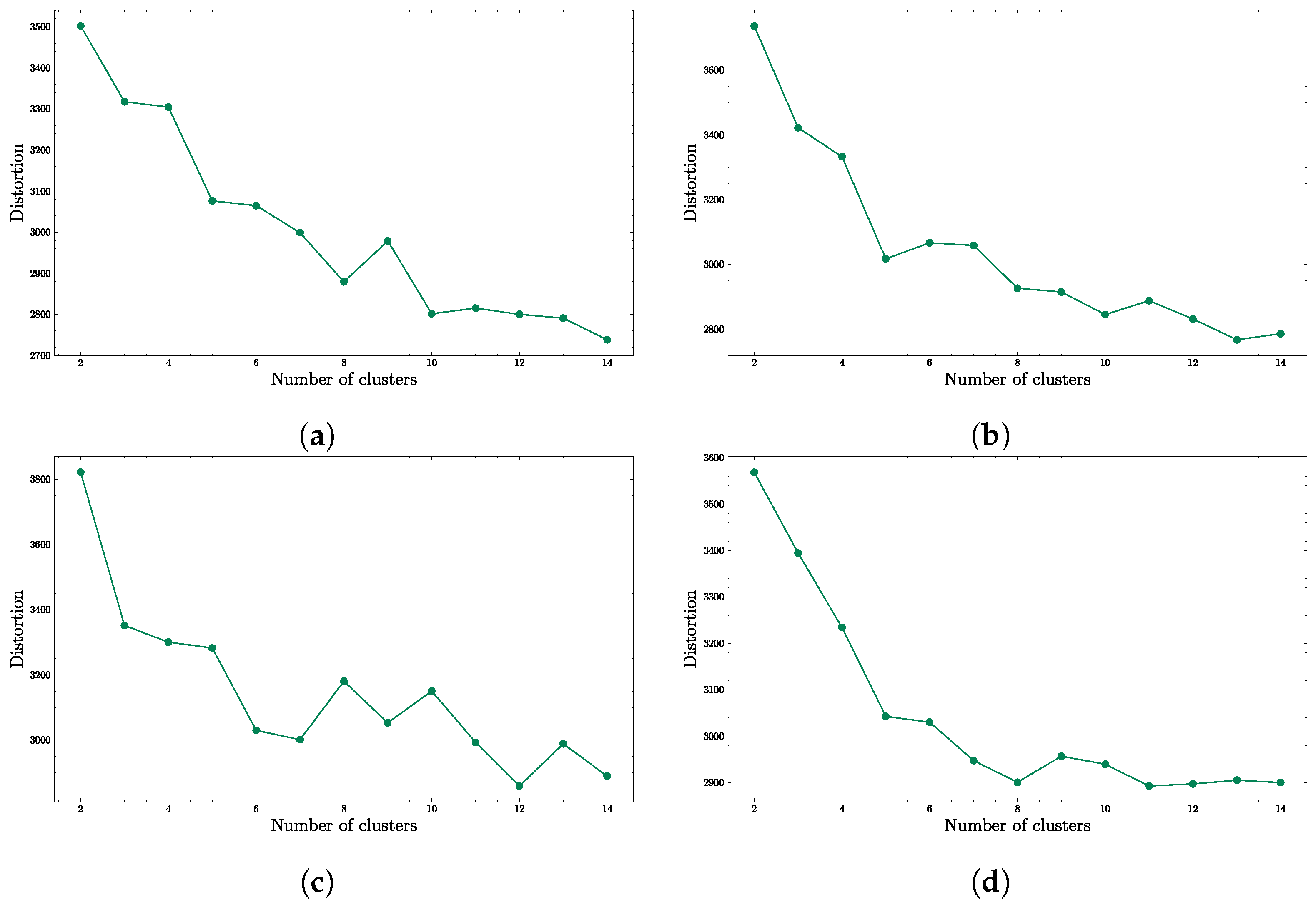
By clustering the normalized feature importance sequences generated from each experiment, different feature importance sequences can be clustered. The number of clusters for each feature’s feature importance sequence is confirmed using the elbow method. According to the elbow theory, as the number of clusters continues to increase, the rate of decrease will tend to stabilize. Thus, we generally select the end value of the steepest segment as the real number of clusters [39]. By visualizing the Euclidean distances obtained from the elbow algorithm at different numbers of clusters, as shown in Figure 5, Figure 5 represents the elbow visualization results of four different experiments, and it can be determined that the optimal number of clusters is 5.
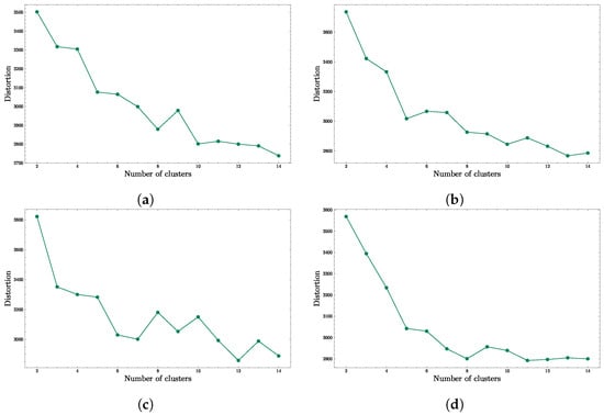
Figure 5.
The determination results of the elbow clustering number under different independent experiments. (a) presents the results with a random seed of 100 and a time step of 180. (b) displays the results with a random seed of 200 and a time step of 180. (c) shows the results with a random seed of 100 and a time step of 240. (d) depicts the results with a random seed of 200 and a time step of 240.
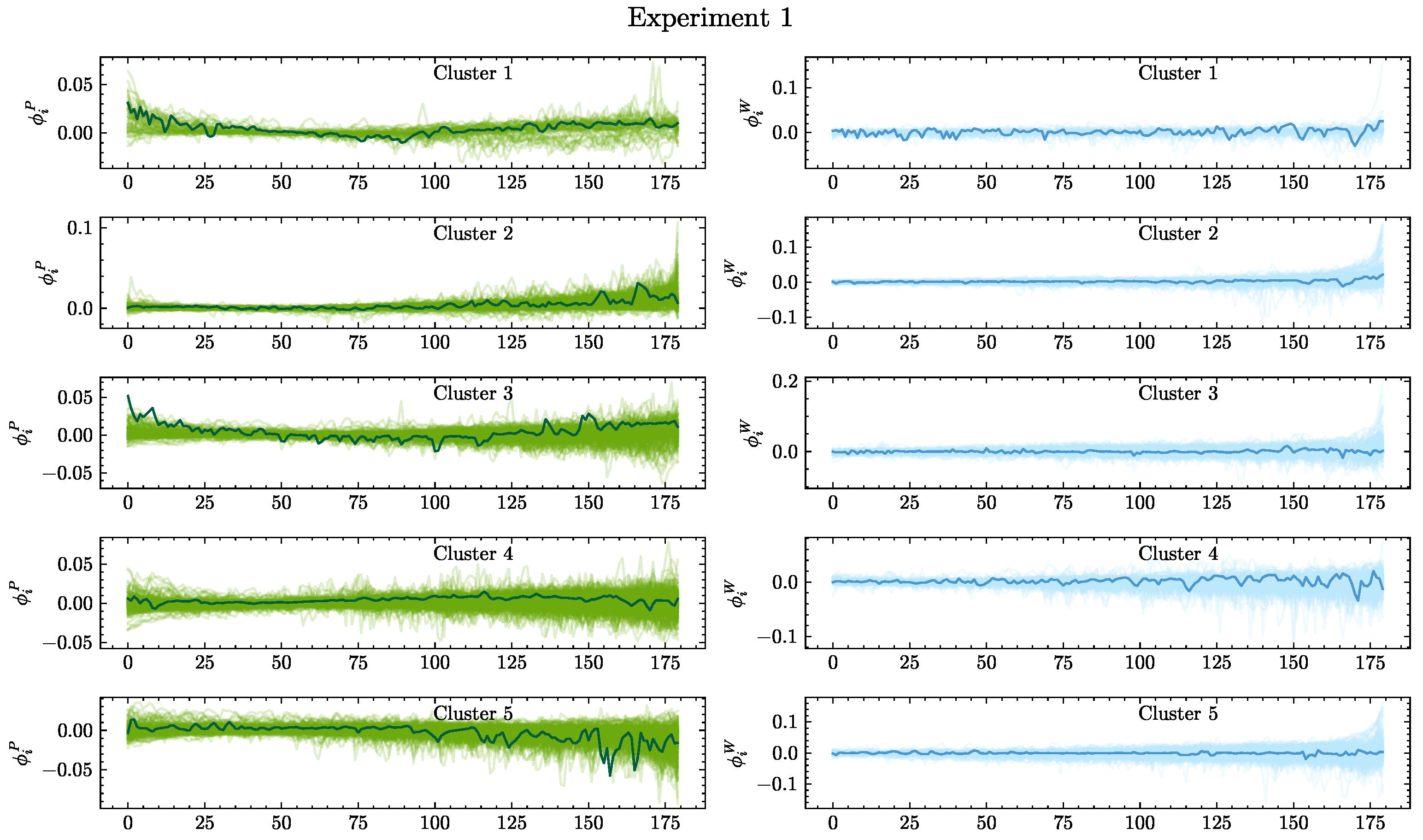
Comparing the number of categories causing marine heatwaves in the coastal areas of China mentioned in the literature [42] and the number of clusters determined by the elbow method, we find that they match the expert’s experience. The normalized feature importance is clustered using the K-Medoids method, and the clustering results are shown in Figure 6.
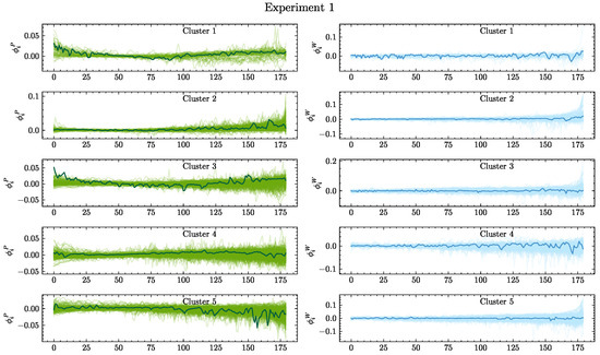
Figure 6.
The results under different cluster categories, where the first column represents the clustering results of sea surface pressure feature importance, and the second column represents the clustering results of 10m wind speed feature importance. Moreover, in each figure, the darkest curve represents the cluster center of each category.
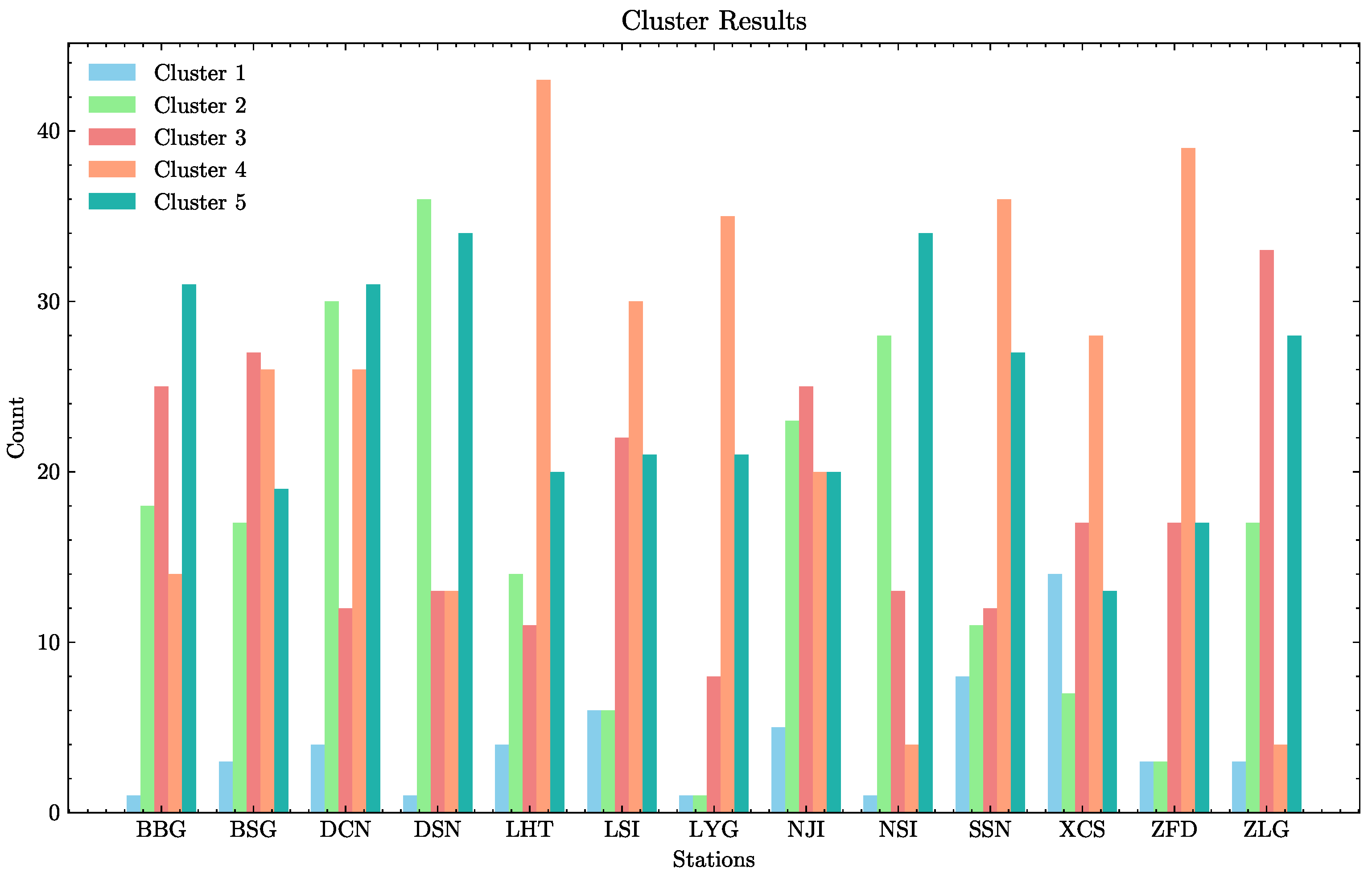
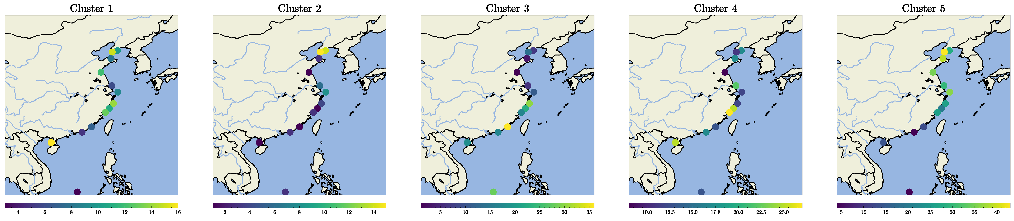
To summarize, we conducted an analysis of the experiment with a random seed of 100 and a time step of 180. The statistical results of 1134 marine heatwave events that occurred at 13 stations from 1982 to 2022 are shown in Table 6, and the number of categories at each station is shown in Figure 7, and the visualization of clustering results on the map is shown in Figure 8. The lighter color represents a greater number of marine heatwave events. From the map, it can be observed that the majority of the first category of marine heatwaves occur along the South China Sea coast, with a few along the other coastal regions of China. The second category predominantly concentrates near the Bohai Strait, the third is focused southwest of the East China Sea and northeast towards the South China Sea, and the fourth category mainly occurs in the East China Sea region. The fifth category primarily takes place near the Bohai Sea and the Yellow Sea.
Table 6.
Comparing existing studies with the interpretable data-driven model shown in Figure 1 of this article, the data used for the model in this article are reanalysis data. The five types of marine heatwave patterns in the table respectively correspond to Nos. 1~5 as identified in experiments.
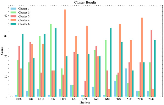
Figure 7.
The number of events in different categories contained at different station.
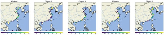
Figure 8.
The number of each type of event in the sea areas of China.
3.3. Interpreted Ocean Mechanisms
By comparing the different clustering results of these 1134 heatwave events, among numerous results, we found representative outputs in these five clustering categories.
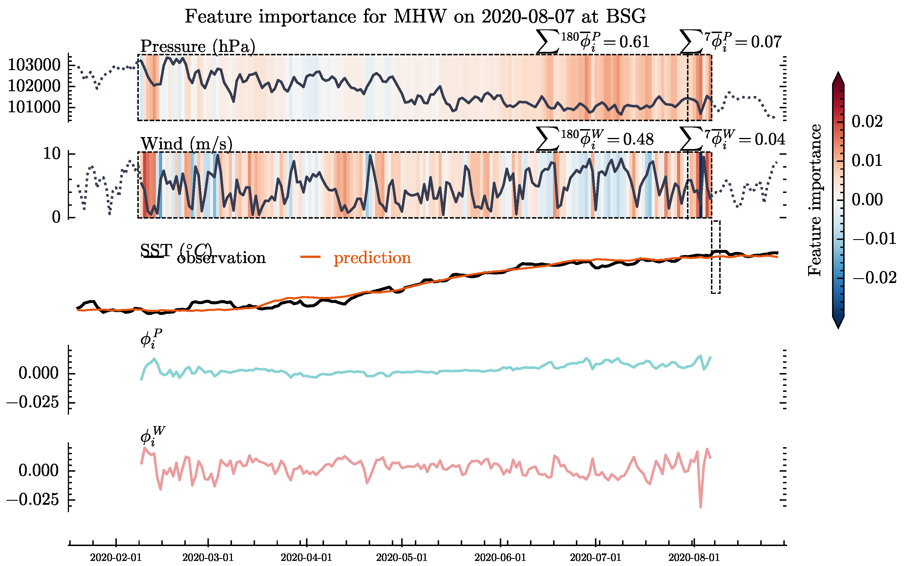
We found a pattern in the marine heatwave event at the BSG station on 7 August 2020. As shown in Figure 9, in the 180 days preceding the marine heatwave event, the persistency of for sea surface pressure and wind speed was consistently . This suggests that the long-term joint effect of sea surface pressure and wind speed induced the marine heatwave event. Comparing with the clustered results, this marine heatwave event pattern belongs to the first category.
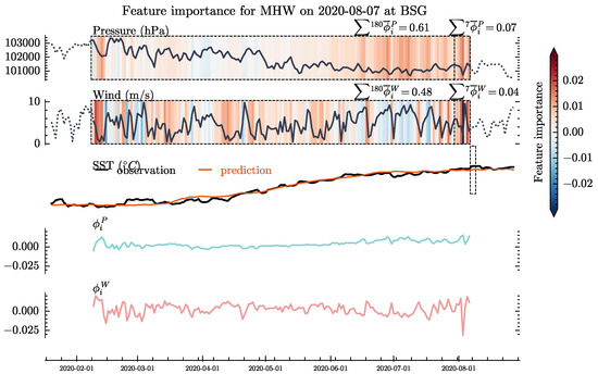
Figure 9.
The marine heatwave event that occurred at BSG station on 7 August 2020, and its corresponding feature importance. The first and second row plots represent the historical data of different points in the 180 days before the marine heatwave event, with colors indicating the feature importance at different time points. The third row plot represents the predicted and observed sea surface temperature values. The fourth and fifth row plots represent the feature importance of pressure and 10 m wind speed, respectively.
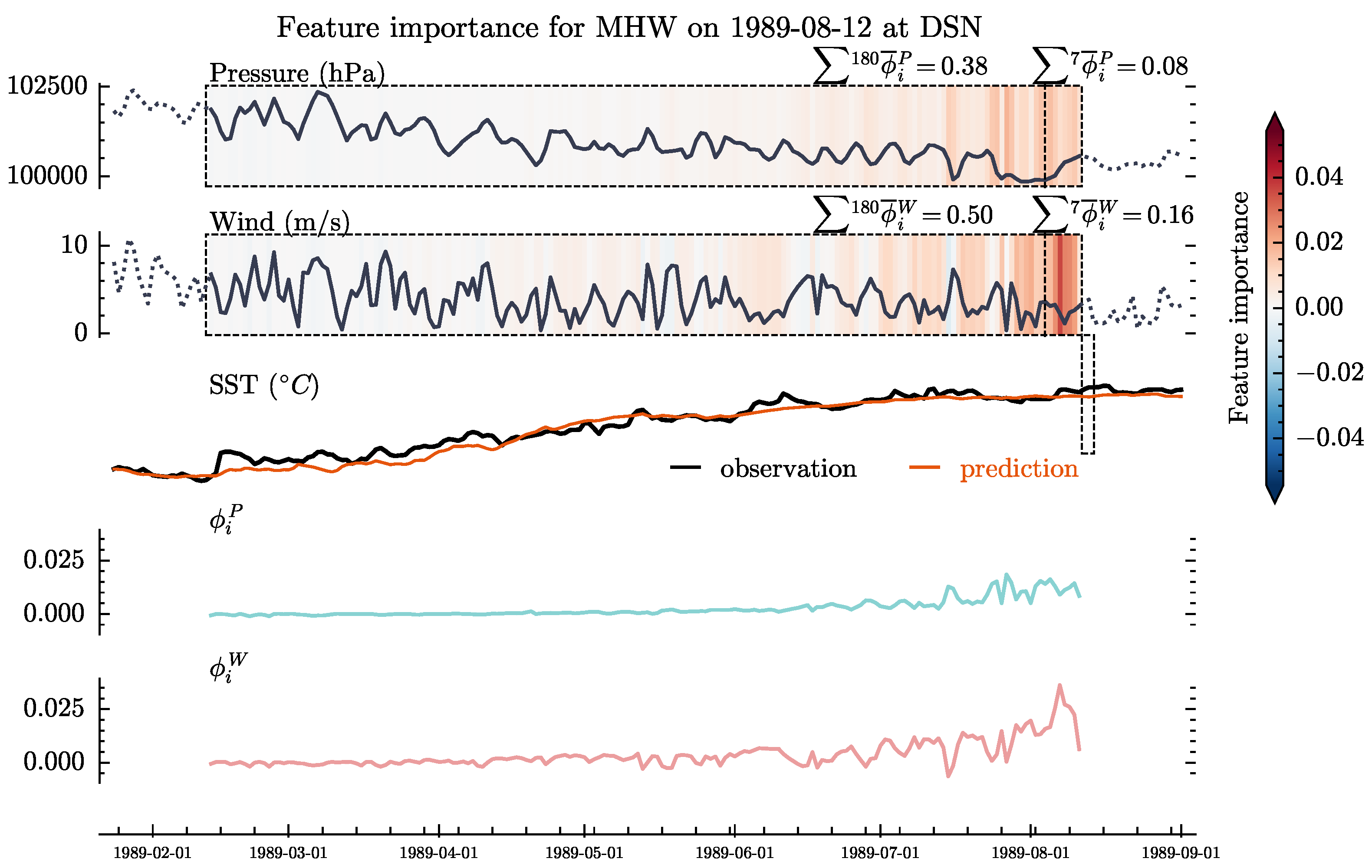
The marine heatwave event on 12 August 1989 at the DSN station represents another pattern. As shown in Figure 10, the significant increase in of sea surface pressure and wind speed occurred just before the marine heatwave event, suggesting that the event was caused by the short-term combined effect of sea surface pressure and wind speed. A comparison with the clustering results reveals that this marine heatwave event pattern belongs to the second category.
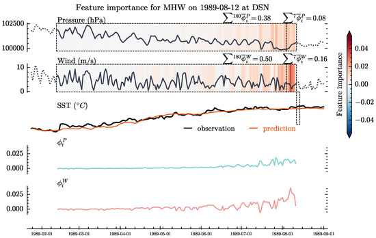
Figure 10.
The marine heatwave event that occurred at DSN station on 12 August 1989, and its corresponding feature importance. The first and second row plots represent the historical data of different points in the 180 days before the marine heatwave event, with colors indicating the feature importance at different time points. The third row plot represents the predicted and observed sea surface temperature values. The fourth and fifth row plots represent the feature importance of pressure and 10 m wind speed, respectively.
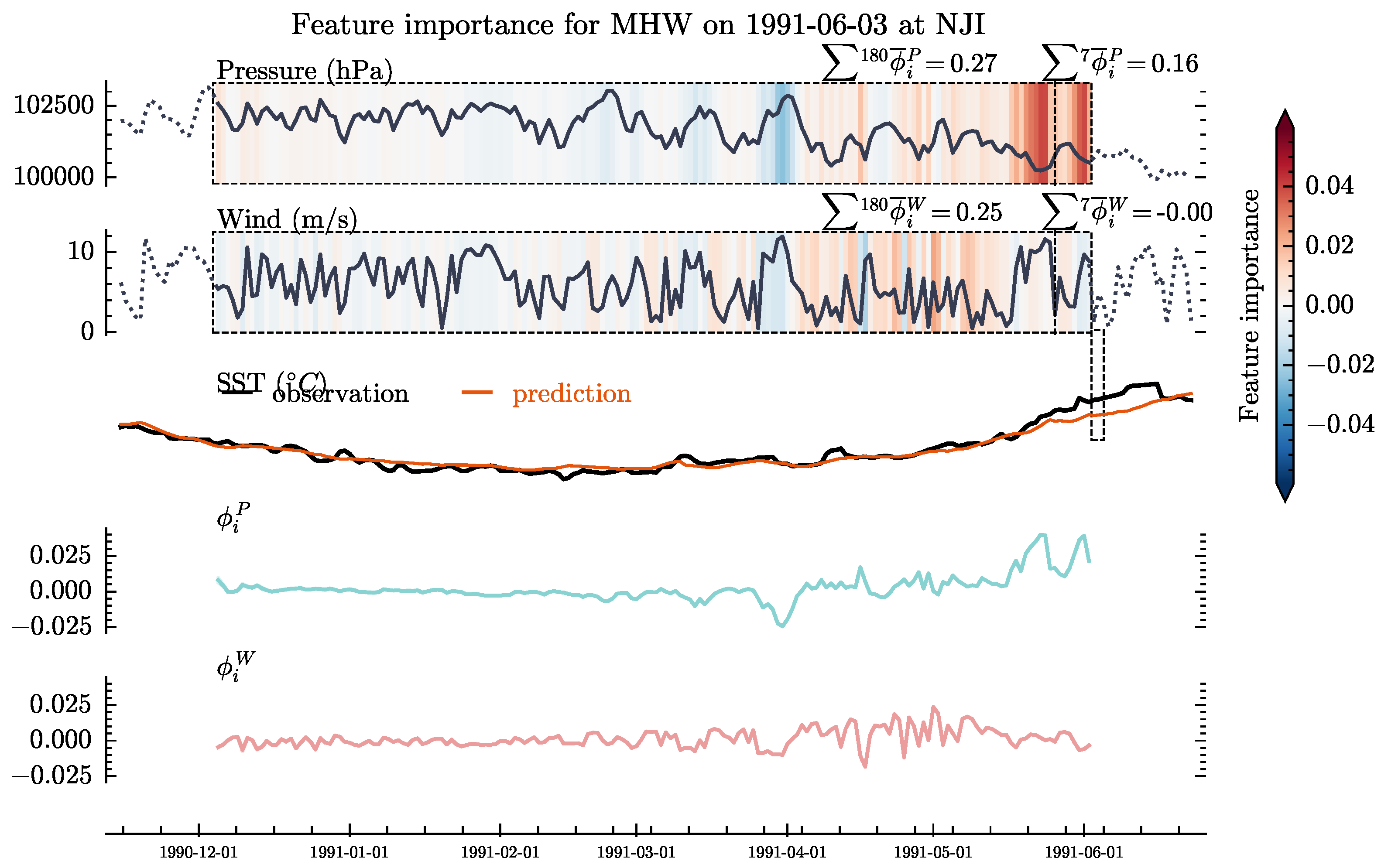
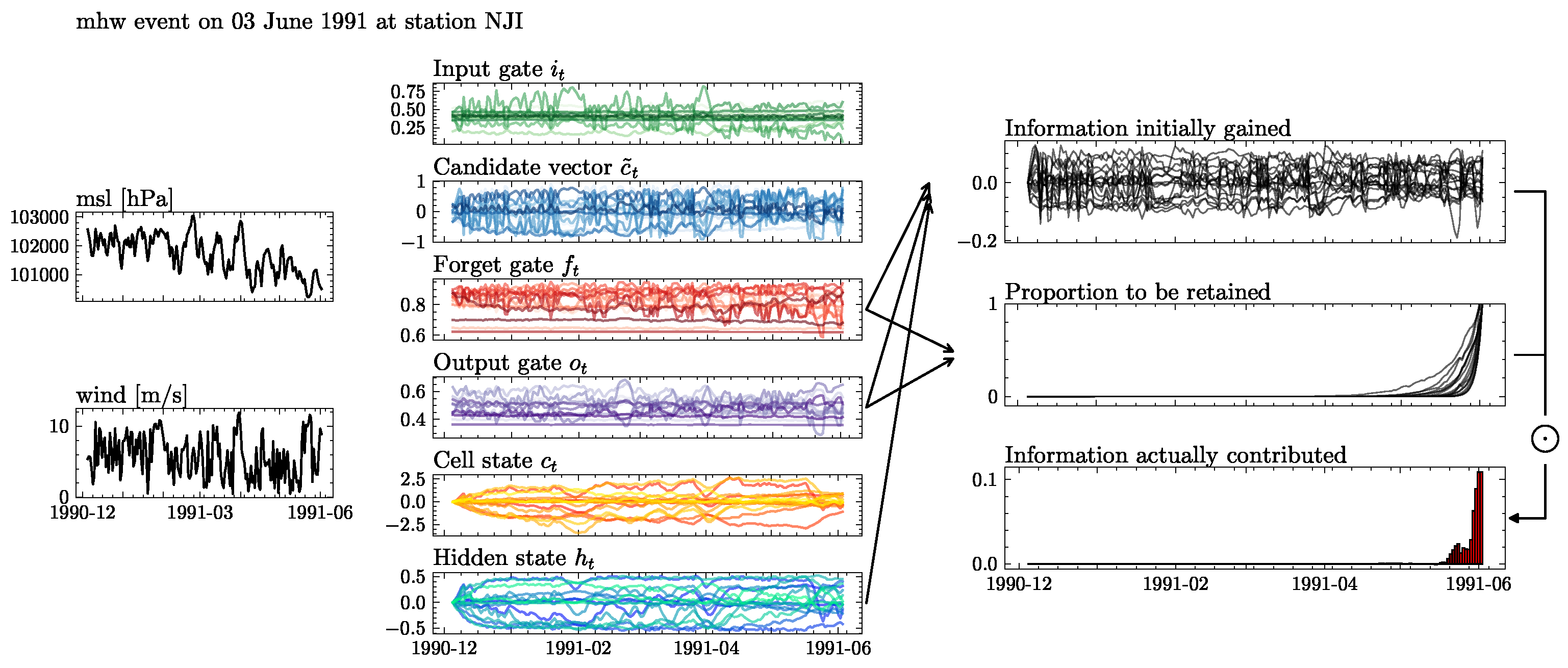
The marine heatwave event on 3 June 1991 at the NJI station corresponds to a pattern illustrated in Figure 11. During the training period, just before the marine heatwave event was about to occur, a significant increase in the of sea surface pressure occurred, with some promoting effects seen in wind speed at more distant points in time. This suggests that the marine heatwave event was caused by the short-term anomaly of sea surface pressure and long-term convergence of the sea surface wind field. Comparison with the clustering results shows that this pattern belongs to the third category.

Figure 11.
The marine heatwave event that occurred at NJI station on 3 June 1991, and its corresponding feature importance. The first and second row plots represent the historical data of different points in the 180 days before the marine heatwave event, with colors indicating the feature importance at different time points. The third row plot represents the predicted and observed sea surface temperature values. The fourth and fifth row plots represent the feature importance of pressure and 10 m wind speed, respectively.
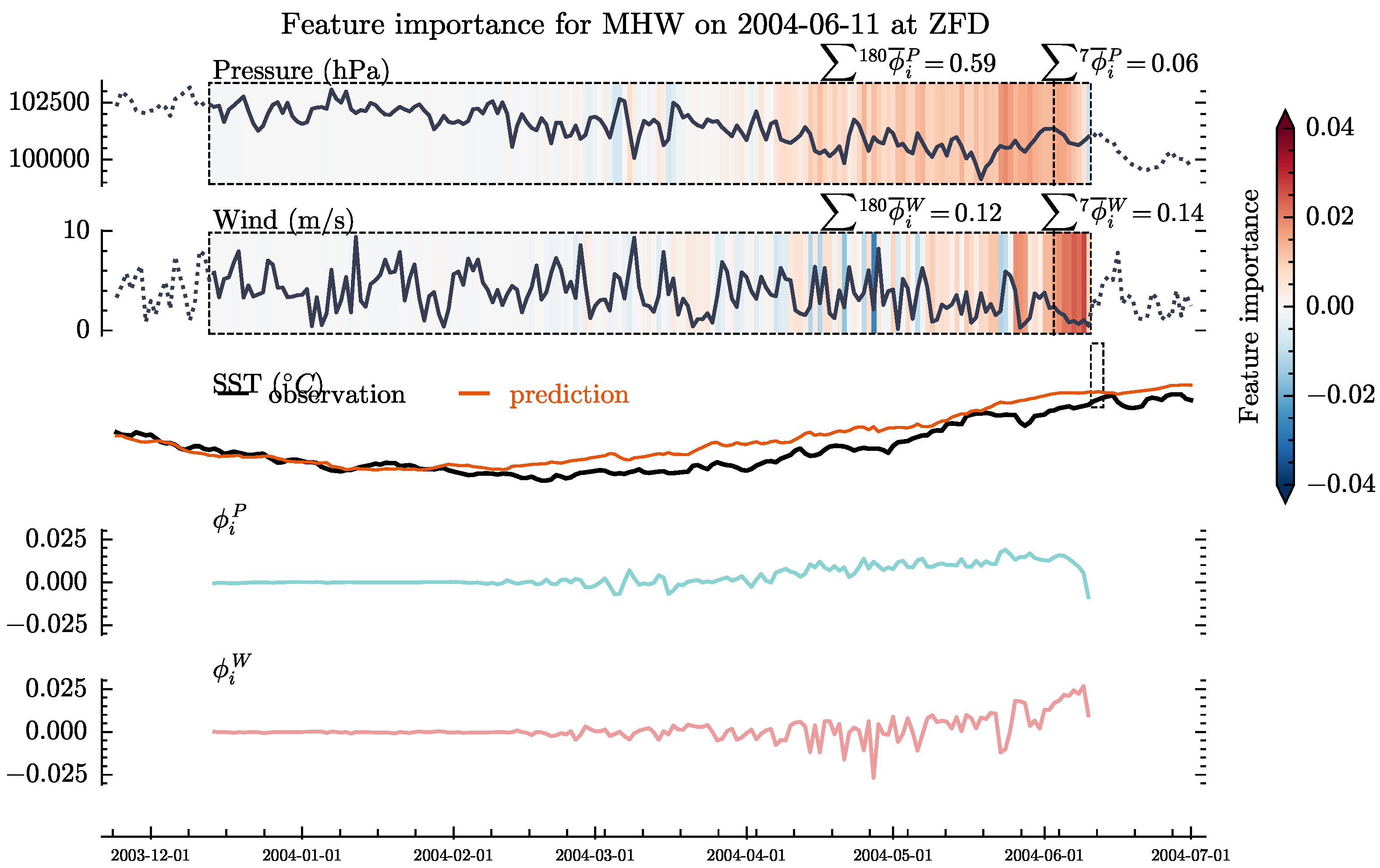
A heatwave event at the ZFD station exhibits a pattern, with Figure 12 showing significant feature analysis obtained for the heatwave event that occurred on 11 June 2004. The of pressure and wind speed remained significant for an extended period before the event. This suggests that atmospheric forces and convergence of the sea surface wind field act in concert, leading to significant changes in wind speed and pressure that trigger the marine heatwave event. The combination of this data with the clustered results shows this marine heatwave event belongs to the fourth category.
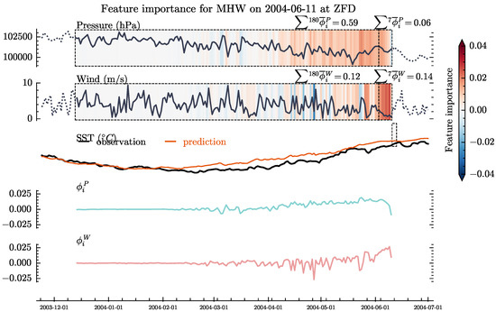
Figure 12.
The marine heatwave event that occurred at ZFD station on 11 June 2004, and its corresponding feature importance. The first and second row plots represent the historical data of different points in the 180 days before the marine heatwave event, with colors indicating the feature importance at different time points. The third row plot represents the predicted and observed sea surface temperature values. The fourth and fifth row plots represent the feature importance of pressure and 10 m wind speed, respectively.
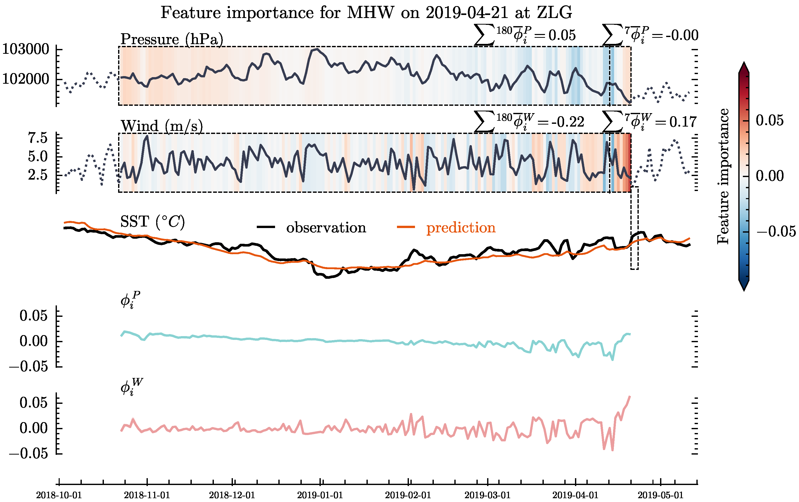
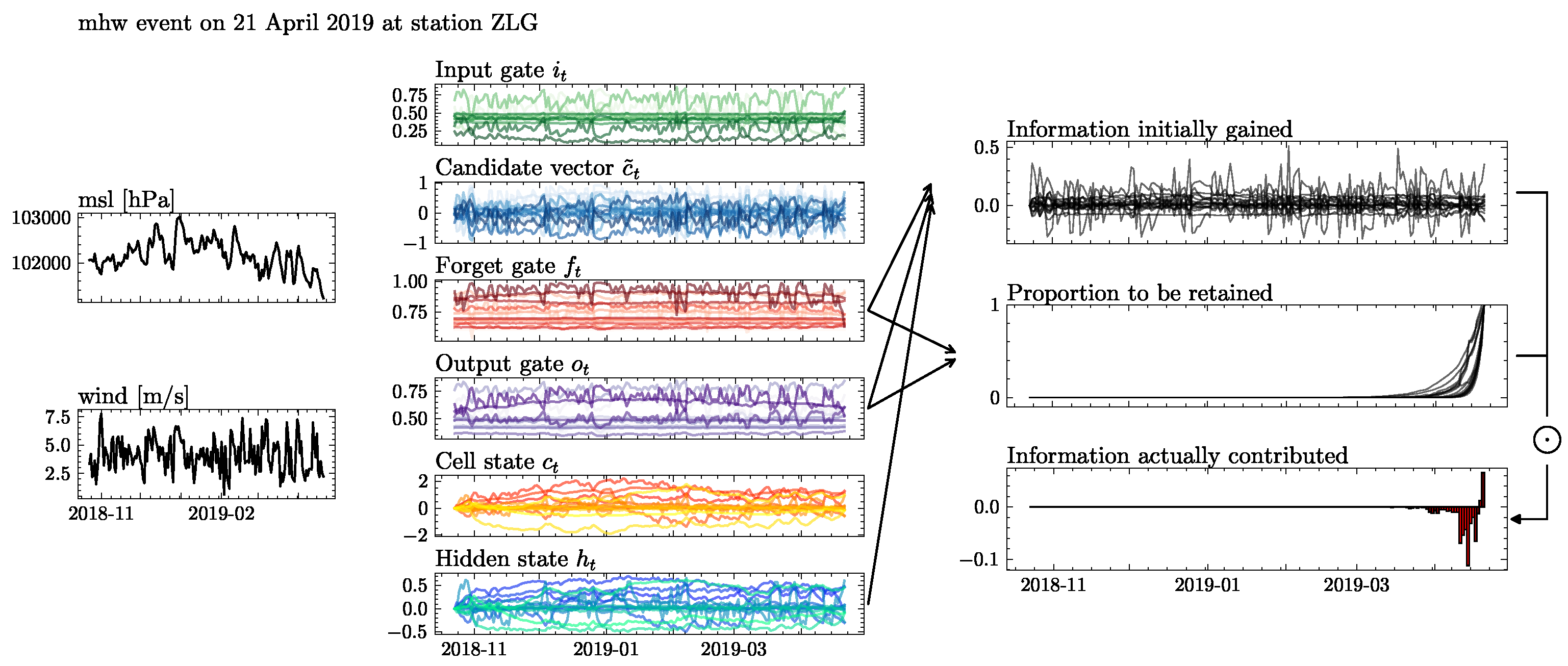
Figure 13 shows the results of feature importance scores for different features of the heatwave event on 21 April 2019, at the ZLG station. The negligible influence of pressure on the event compared with wind speed is evident, and only the values of wind speed near the event marked a significant upward trend, while values of wind speed at other times had hardly any noticeable effect. The pattern analysis indicates that this heatwave event was likely triggered by recent convergence of the sea surface wind field, which can cause convergence and intensification of warm surface water and Ekman downwelling, leading to continued subsurface ocean warming and the subsurfacemarine heatwave phenomenon. In this case, while the previous wind speed in the station area might more or less intensify the heatwave event, the recent convergence of the sea surface wind field made an absolute contribution to the event occurrence. Comparison with the clustering results reveals that this marine heatwave event belongs to the fifth category.
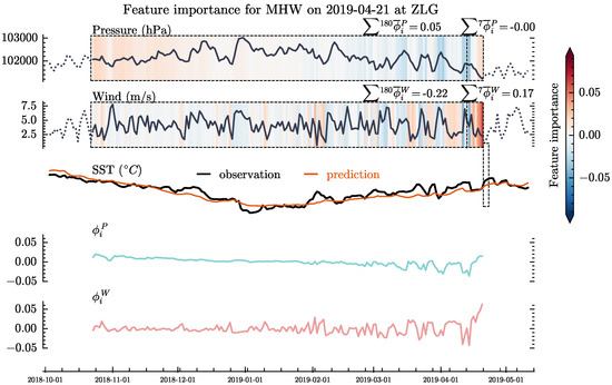
Figure 13.
The marine heatwave event that occurred at ZLG station on 21 Apirl 2019, and its corresponding feature importance. The first and second row plots represent the historical data of different points in the 180 days before the marine heatwave event, with colors indicating the feature importance at different time points. The third row plot represents the predicted and observed sea surface temperature values. The fourth and fifth row plots represent the feature importance of pressure and 10m wind speed, respectively.
3.4. Decomposing Internal Signals of LSTM with AD
The previously introduced AD method was used for exploring the internal behavior of the LSTM model. As an illustrative example, Figure 14 and Figure 15 respectively plot the internal signals in the LSTM model when predicting the marine heat wave events at the NJI station on 3 June 1991, and at the ZLG station on 21 April 2019. In these figures, the first column visualizes the sea surface pressure and wind speed 180 days prior, which are used to predict the sea surface temperature. The second column visualizes the evolution of six internal variables within the corresponding LSTM model, including the input gate, candidate vectors, forget gate, output gate, cell state, and hidden state. However, the visualization of these hidden signals is quite chaotic, making it difficult to obtain effective information. The third column shows the information extracted from the second column using the AD method, providing clearer clues to the behavior of the LSTM model.
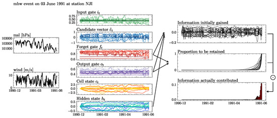
Figure 14.
Performed AD analysis on the marine heatwave event that occurred at the NJI station on 3 June 1991.
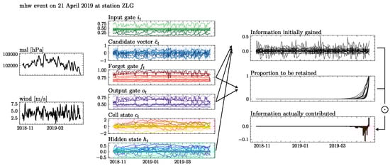
Figure 15.
Performed AD analysis on the marine heatwave event that occurred at the NJI station on 21 April 2009.
The first two images in the third column of Figure 14 and Figure 15 show the breakdown of the information contributing to the final model decision at each timestep, that is, the original information obtained at each step and the proportion to be retained towards the final step. The zero values in the middle image mean that the initial information obtained by the unit at the corresponding timestep will be completely forgotten. The image below represents the weighted sum of the element-wise multiplication of the above two items, indicating the information ultimately contributed at each timestep. The total contribution of information across all timesteps is the final output (i.e., sea surface temperature prediction).
The analysis of internal signals shown in Figure 14 reveals that for the sea surface temperature prediction at the NJI station, the long-term memory in several hidden units is activated. As a result, previous sea surface pressure is partially retained to assist the prediction.
Furthermore, as shown in Figure 15, previous inputs can have a relatively long-term impact, principally due to memory retained in a hidden unit, the degree of which partly depends on the magnitude of the sea surface pressure. In contrast, the contribution of the recent wind speed to the output may be triggered by information obtained near the final timestep, as evidenced by the last segment of the line representing temperature observations in the first image of the third column of Figure 15.
4. Discussion
4.1. Interpretation of Results
In Experiment One, our aim was to validate our hypothesis and evaluate the performance of the new method. First, we collected a dataset consisting of 1000 samples. Each sample had a set of input features and corresponding labels. We used this dataset to train our models and used traditional methods as a benchmark for comparison. To validate our hypothesis, we used the Expected Gradient (EG) method and Additive Decomposition (AD) method to interpret and analyze the model’s decision-making process. We obtained the interpretation results of the EG method by calculating the gradient of each input feature, and we analyzed the flow of information in the LSTM network using the AD method. Through these methods, we gleaned some insights and conclusions about the model’s behavior. To evaluate the performance of the new method, we conducted both quantitative and qualitative assessments. In the quantitative assessment, we compared the performance of the EG and AD methods in interpretation and prediction accuracy. We calculated their scores on various metrics and performed statistical analyses. In the qualitative assessment, we invited some domain experts to evaluate the interpretation results of the new method and collected their feedback and opinions. The experimental results showed that the EG and AD methods performed well in interpreting model decisions and predicting accuracy. The EG method provided a clear explanation of the contribution of each input feature, revealing the importance of features. The AD method delved deep into the workings of the LSTM network, revealing the model’s mechanisms when dealing with sequential information. The experts’ evaluations also corroborated the interpretability and credibility of these methods. In summary, No.1 experiment validated our hypothesis and proved the effectiveness of the Expected Gradient method and Additive Decomposition method in interpreting neural network behavior. These methods provided us with deep insights into the model’s decision-making process and offered potential for improving interpretability and credibility. In subsequent experiments, we will further explore the application and advancement of these methods to achieve superior interpretability.
4.2. Compared with Existing Research
Hu and Li [42] discovered several patterns in the coastal areas of China. The first is that marine heatwave events in the South China Sea primarily occur in the Nansha Islands and the Gulf of Tonkin, related to the weakening of the East Asian winter monsoon and the strengthening of the West Pacific subtropical high pressure and South China Sea high pressure. The second pattern involves an abnormal strengthening of the Northwest Pacific subtropical high-pressure system in summer, an increase in solar shortwave radiation, a weakening of Walker circulation, a reduction in latent heat release at the sea surface, an increase in net heat flux, an extension of the cyclone westward leading to an anomaly in the low-latitude easterlies, the weakening of the southwest summer monsoon, and a reduction or even disappearance of upwelling in the central and western regions of the South China Sea, forming strong basin-scale marine heatwaves in summer. The third pattern appears during El Niño events when the winter cyclonic anomaly in the Northwest Pacific weakens the East Asian winter monsoon; the south wind is relatively strong, increasing the northward transport of warm surface water and reducing the cold surge west of Hainan Island, resulting in marine heatwaves in the Gulf of Tonkin. The fourth is that the South China Sea’s high pressure extends westward during El Niño warm events, inhibiting the evaporation process, enhancing the shortwave solar radiation received by the ocean surface, and weakening the wind field, thereby forming marine heatwaves. The fifth pattern is in the East China Sea and Southern Yellow Sea regions, where marine heatwave events are mainly influenced by anomalies in the East Asian summer monsoon, Northwest Pacific anomalous anti-cyclonic circulation, and local ocean dynamic processes. Another pattern involves an anomalous anti-cyclonic circulation over the Northwest Pacific leading to increased sea surface temperatures in the Eastern Indian Ocean equatorial region and the Western Pacific equatorial region, which, due to strong adiabatic sinking motion and solar shortwave radiation, causes extreme high-temperature events in the East China Sea; on the other hand, it also leads to extreme high-temperature events in the East China Sea by enhancing the transport of warm Kuroshio water towards the East China Sea region. It can be observed that there is an overlap between the patterns found in the research and the models discovered by the article. Table 6 lists some studies that coincide with the marine heatwave mechanisms identified in this experiment.
Research has shown that the South China Sea is dominated by the East Asian monsoon, with a warm and humid southwest wind in the summer [47]. Blocked by the mountains on the eastern coast of the Indo-China Peninsula, the southwest wind surges past the southern end of this range, forming a strong wind jet near southeastern Vietnam [48]. Driven by the early summer monsoon wind, offshore Ekman transport brings up cold subsurface water to the surface near the coast [48,49]. As the wind stress extends eastward, the cold sea surface area continues to expand in July and August into the central part of South China Sea; this phenomenon is known as the midsummer cooling effect. Notably, the cold water range in the upwelling zone of the western–central South China Sea continues to expand, reaching its maximum area in August, while the upwelling zone in the northern South China Sea displays the oppositional trend. In addition, the warm sea surface range in the Gulf of Tonkin enlarges from June to August.
As shown in Figure 16, the significance of wind speed features markedly increases near the occurrence of marine heatwaves, which verifies our hypothesis and illustrates the pertinence of the Northern Bay marine heatwave generation pattern studied.
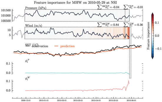
Figure 16.
The marine heatwave event that occurred at NSI station on 29 May 2010, and its corresponding feature importance. The first and second row plots represent the historical data of different points in the 180 days before the marine heatwave event, with colors indicating the feature importance at different time points. The third row plot represents the predicted and observed sea surface temperature values. The fourth and fifth row plots represent the feature importance of pressure and 10m wind speed, respectively.
4.3. Limitations of the Model
Although this study assessed the interpretability of different input features for marine heatwave patterns, it is difficult to discern some complex information using existing expert experiences. Some evidence suggests that LSTM (Long Short-Term Memory) models can effectively interpret results [50], but we believe that directly associating the LSTM network’s memory with marine heatwave patterns may not necessarily be reliable. Marine heatwaves are discrete, persistent abnormal warming events occurring in the ocean, and there are certain teleconnections. Current research shows that the occurrence of marine heatwaves is often closely related to large-scale ocean climate modes, especially low-frequency climate modes (such as ENSO). Therefore, different from the concept of how marine heatwaves form, the internal dynamics in LSTM units may have their own principles to reproduce the nonlinear relationships and time dependence in the variables related to marine heatwaves. We hope that future research will apply advanced interpretability and visualization techniques to unveil the mystery of LSTM memory, such as fully understanding the reactions between input features and hidden memories, which might possibly reveal causal relationships we have yet to recognize.
5. Conclusions
In this paper, we propose an innovative approach to explore marine heatwave patterns through deep learning. We have successfully combined the robustness of complex deep learning models with interpretive tools to provide a deeper and more interpretable understanding of marine heatwave patterns. In this paper, a LSTM model identifies nonlinear relationships between 10m wind speeds, sea surface pressure, and sea surface temperatures at 13 coastal sites in China. Then, using 10m wind speeds and sea surface pressure, the model predicts sea surface temperatures. The efficacy of the model is assessed through the MSE and the RMSE of these predictions, which indicate good predictive performance. Following the definition of marine heatwaves, the paper identifies marine heatwave events and applies feature importance score clustering analysis to characterize the events. This analysis has revealed five patterns contributing to the occurrence of marine heatwaves along the Chinese coast. In addressing these marine heatwave events, we employ two interpretable methods for explanation and compare the outcomes with existing theoretical research, finding a congruence. We demonstrated that the expected gradient method mentioned in the paper reveals different patterns of feature importance and reveals different performances of the LSTM networks in retaining and discarding information when simulating different types of marine heatwaves through additive decomposition methods. This deep learning framework can effectively reveal complex and non-linear patterns of marine heatwaves. The critical breakthrough of this method is that the features and parameters used to generate predictive results can be explained easily, making it a powerful tool for researchers to fully understand such initially intricate phenomena.
We observed that due to the dynamic and adaptive nature provided by deep learning, this method shows a robust capability in dealing with the vulnerability and anomalies of marine heatwaves, which are aspects that traditional models fail to grasp. This breakthrough method has opened new possibilities in analyzing and simulating the complexity and uncertainty of marine heatwaves. However, we recognize that there are some challenges and limitations in the development of models, including the quality and representation of data, and the transparency and interpretability of deep learning models. These issues require further research to increase the application value and practicality of the model.
In summary, our research indicates that deep learning-based predictions on marine heatwave patterns provide a tool with enormous potential. In future research, we look forward to further optimizing the model and applying this framework to larger environmental datasets to more accurately predict and understand marine heatwaves and their impact on the global climate. Moreover, this framework also provides a new, interpretable model for applying deep learning to other complex issues in environmental science and climate research. Although our method yielded good results, it still has limitations. Since EG feature importance scores are mostly chaotic and unordered, they may not provide a good explanation method, and the fact that the patterns that the experiment generated are uninterpretable also poses directions for future research in marine heatwave patterns in Earth science. Next, we anticipate extending this research method to predictions and analysis of other marine phenomena and climate patterns, further promoting the application of deep learning in environmental science.
Author Contributions
Conceptualization, Q.H. and Z.Z.; methodology, Q.H. and Z.Z.; software, Z.Z.; validation, Q.H. and Z.Z.; resources, D.Z. and Z.Z.; data curation, Z.Z.; writing—original draft preparation, Z.Z.; writing—review and editing, Q.H., W.S. and D.H.; funding acquisition, Q.H. All authors have read and agreed to the published version of the manuscript.
Funding
This research was funded by the National Key Research and Development Program of China (No. 2021YFC3101602), National Natural Science Foundation of China (No. 42376194) and the Young Scientists Fund of the National Natural Science Foundation of China (No. 42106190).
Institutional Review Board Statement
Not applicable.
Informed Consent Statement
Not applicable.
Data Availability Statement
The data presented in this study are available upon request from the corresponding author. For the experimental code of this paper you can contact the author’s e-mail. E-mail: zhujerry1998@163.com.
Acknowledgments
We would like to thank the anonymous reviewers for their insightful comments and substantial help in improving this paper.
Conflicts of Interest
The authors declare no conflicts of interest.
References
- Herring, S.C.; Christidis, N.; Hoell, A.; Stott, P.A. Explaining Extreme Events of 2020 from a Climate Perspective. Bull. Am. Meteorol. Soc. 2022, 103, S1–S129. [Google Scholar] [CrossRef]
- Pearce, A.F.; Feng, M. The rise and fall of the “marine heat wave” off Western Australia during the summer of 2010/2011. J. Mar. Syst. 2013, 111–112, 139–156. [Google Scholar] [CrossRef]
- Frölicher, T.L.; Fischer, E.M.; Gruber, N. Marine heatwaves under global warming. Nature 2018, 560, 360–364. [Google Scholar] [CrossRef] [PubMed]
- Yao, Y.; Wang, C. Marine heatwaves and cold-spells in global coral reef zones. Prog. Oceanogr. 2022, 209, 102920. [Google Scholar] [CrossRef]
- Fredston, A.L.; Cheung, W.W.L.; Frölicher, T.L.; Kitchel, Z.J.; Maureaud, A.A.; Thorson, J.T.; Auber, A.; Mérigot, B.; Palacios-Abrantes, J.; Palomares, M.L.D.; et al. Marine heatwaves are not a dominant driver of change in demersal fishes. Nature 2023, 621, 324–329. [Google Scholar] [CrossRef]
- Masson-Delmotte, V.; Zhai, P.; Pirani, A.; Connors, S.L.; Péan, C.; Berger, S.; Caud, N.; Chen, Y.; Goldfarb, L.; Gomis, M.I. Climate change 2021: The physical science basis. In Contribution of Working Group I to the Sixth Assessment Report of the Intergovernmental Panel on Climate Change; Cambridge University Press: Cambridge, UK, 2021; Volume 2. [Google Scholar]
- Hu, S.; Sprintall, J.; Guan, C.; McPhaden, M.J.; Wang, F.; Hu, D.; Cai, W. Deep-reaching acceleration of global mean ocean circulation over the past two decades. Sci. Adv. 2020, 6, eaax7727. [Google Scholar] [CrossRef] [PubMed]
- Hu, S.; Lu, X.; Li, S.; Wang, F.; Guan, C.; Hu, D.; Xin, L.; Ma, J. Multi-decadal trends in the tropical Pacific western boundary currents retrieved from historical hydrological observations. Sci. China Earth Sci. 2021, 64, 600–610. [Google Scholar] [CrossRef]
- Shi, J.R.; Talley, L.D.; Xie, S.P.; Peng, Q.; Liu, W. Ocean warming and accelerating Southern Ocean zonal flow. Nat. Clim. Chang. 2021, 11, 1090–1097. [Google Scholar] [CrossRef]
- Balaguru, K.; Foltz, G.R.; Leung, L.R.; Emanuel, K.A. Global warming-induced upper-ocean freshening and the intensification of super typhoons. Nat. Commun. 2016, 7, 13670. [Google Scholar] [CrossRef]
- Martínez-Moreno, J.; Hogg, A.M.; England, M.H.; Constantinou, N.C.; Kiss, A.E.; Morrison, A.K. Global changes in oceanic mesoscale currents over the satellite altimetry record. Nat. Clim. Chang. 2021, 11, 397–403. [Google Scholar] [CrossRef]
- Hobday, A.J.; Alexander, L.V.; Perkins, S.E.; Smale, D.A.; Straub, S.C.; Oliver, E.C.; Benthuysen, J.A.; Burrows, M.T.; Donat, M.G.; Feng, M.; et al. A hierarchical approach to defining marine heatwaves. Prog. Oceanogr. 2016, 141, 227–238. [Google Scholar] [CrossRef]
- Reichstein, M.; Camps-Valls, G.; Stevens, B.; Jung, M.; Denzler, J.; Carvalhais, N.; Prabhat. Deep learning and process understanding for data-driven Earth system science. Nature 2019, 566, 195–204. [Google Scholar] [CrossRef] [PubMed]
- Zhang, Q.; Wang, H.; Dong, J.; Zhong, G.; Sun, X. Prediction of Sea Surface Temperature Using Long Short-Term Memory. IEEE Geosci. Remote Sens. Lett. 2017, 14, 1745–1749. [Google Scholar] [CrossRef]
- Ham, Y.G.; Kim, J.H.; Luo, J.J. Deep learning for multi-year ENSO forecasts. Nature 2019, 573, 568–572. [Google Scholar] [CrossRef]
- Ham, Y.G.; Kim, J.H.; Kim, E.S.; On, K.W. Unified deep learning model for El Niño/Southern Oscillation forecasts by incorporating seasonality in climate data. Sci. Bull. 2021, 66, 1358–1366. [Google Scholar] [CrossRef]
- Prasad, A.; Sharma, S.; Agarwal, H. Forecasting Marine Heatwaves Using Machine Learning. 2022; preprint. [Google Scholar] [CrossRef]
- Liang, Y.; Li, S.; Yan, C.; Li, M.; Jiang, C. Explaining the black-box model: A survey of local interpretation methods for deep neural networks. Neurocomputing 2021, 419, 168–182. [Google Scholar] [CrossRef]
- Samek, W.; Müller, K.R. Towards Explainable Artificial Intelligence. In Explainable AI: Interpreting, Explaining and Visualizing Deep Learning; Springer: Berlin/Heidelberg, Germany, 2019; Volume 11700, pp. 5–22. ISBN 9783030289539. [Google Scholar] [CrossRef]
- Adadi, A.; Berrada, M. Peeking Inside the Black-Box: A Survey on Explainable Artificial Intelligence (XAI). IEEE Access 2018, 6, 52138–52160. [Google Scholar] [CrossRef]
- Guidotti, R.; Monreale, A.; Ruggieri, S.; Turini, F.; Giannotti, F.; Pedreschi, D. A Survey of Methods for Explaining Black Box Models. ACM Comput. Surv. 2019, 51, 1–42. [Google Scholar] [CrossRef]
- Arras, L.; Arjona-Medina, J.; Widrich, M.; Montavon, G.; Gillhofer, M.; Müller, K.R.; Hochreiter, S.; Samek, W. Explaining and Interpreting LSTMs. In Explainable AI: Interpreting, Explaining and Visualizing Deep Learning; Springer International Publishing: Cham, Switzerland, 2019; Volume 11700, pp. 211–238. ISBN 9783030289539. [Google Scholar] [CrossRef]
- Ming, Y.; Cao, S.; Zhang, R.; Li, Z.; Chen, Y.; Song, Y.; Qu, H. Understanding Hidden Memories of Recurrent Neural Networks. In Proceedings of the 2017 IEEE Conference on Visual Analytics Science and Technology (VAST), Phoenix, AZ, USA, 3–6 October 2017; pp. 13–24. [Google Scholar] [CrossRef]
- Strobelt, H.; Gehrmann, S.; Pfister, H.; Rush, A.M. LSTMVis: A Tool for Visual Analysis of Hidden State Dynamics in Recurrent Neural Networks. IEEE Trans. Vis. Comput. Graph. 2018, 24, 667–676. [Google Scholar] [CrossRef]
- Jiang, S.; Zheng, Y.; Wang, C.; Babovic, V. Uncovering Flooding Mechanisms Across the Contiguous United States Through Interpretive Deep Learning on Representative Catchments. Water Resour. Res. 2022, 58, e2021WR030185. [Google Scholar] [CrossRef]
- Erion, G.; Janizek, J.D.; Sturmfels, P.; Lundberg, S.M.; Lee, S.I. Improving performance of deep learning models with axiomatic attribution priors and expected gradients. Nat. Mach. Intell. 2021, 3, 620–631. [Google Scholar] [CrossRef]
- Du, M.; Liu, N.; Yang, F.; Ji, S.; Hu, X. On Attribution of Recurrent Neural Network Predictions via Additive Decomposition. In Proceedings of the The World Wide Web Conference, San Francisco, CA, USA, 13–17 May 2019; pp. 383–393. [Google Scholar] [CrossRef]
- Reynolds, R.W.; Smith, T.M.; Liu, C.; Chelton, D.B.; Casey, K.S.; Schlax, M.G. Daily High-Resolution-Blended Analyses for Sea Surface Temperature. J. Clim. 2007, 20, 5473–5496. [Google Scholar] [CrossRef]
- Hersbach, H.; Rosnay, P.; Schepers, D.; Simmons, A.; Soci, C.; Abdalla, S.; Alonso, M.; Balmaseda; Balsamo, G.; Bechtold, P.; et al. Operational Global Reanalysis: Progress, Future Directions and Synergies with NWP. 2018. Available online: https://www.ecmwf.int/en/elibrary/80922-operational-global-reanalysis-progress-future-directions-and-synergies-nwp (accessed on 22 July 2023).
- Sherstinsky, A. Fundamentals of Recurrent Neural Network (RNN) and Long Short-Term Memory (LSTM) network. Phys. D Nonlinear Phenom. 2020, 404, 132306. [Google Scholar] [CrossRef]
- Kingma, D.P.; Ba, J. Adam: A Method for Stochastic Optimization. arXiv 2014, arXiv:1412.6980. [Google Scholar]
- Oliver, E.C.; Benthuysen, J.A.; Darmaraki, S.; Donat, M.G.; Hobday, A.J.; Holbrook, N.J.; Schlegel, R.W.; Sen Gupta, A. Marine Heatwaves. Annu. Rev. Mar. Sci. 2021, 13, 313–342. [Google Scholar] [CrossRef]
- Sorte, C.J.B.; Fuller, A.; Bracken, M.E.S. Impacts of a simulated heat wave on composition of a marine community. Oikos 2010, 119, 1909–1918. [Google Scholar] [CrossRef]
- Marbà, N.; Jordà, G.; Agustí, S.; Girard, C.; Duarte, C.M. Footprints of climate change on Mediterranean Sea biota. Front. Mar. Sci. 2015, 2, 56. [Google Scholar] [CrossRef]
- Sundararajan, M.; Taly, A.; Yan, Q. Axiomatic Attribution for Deep Networks. 2017. Available online: https://proceedings.mlr.press/v70/sundararajan17a.html (accessed on 5 August 2023).
- Lundberg, S.M.; Lee, S.I. A Unified Approach to Interpreting Model Predictions. arXiv 2017, arXiv:1705.07874. [Google Scholar]
- Petitjean, F.; Ketterlin, A.; Gançarski, P. A global averaging method for dynamic time warping, with applications to clustering. Pattern Recognit. 2011, 44, 678–693. [Google Scholar] [CrossRef]
- Sakoe, H.; Chiba, S. Dynamic programming algorithm optimization for spoken word recognition. IEEE Trans. Acoust. Speech Signal Process. 1978, 26, 43–49. [Google Scholar] [CrossRef]
- Kodinariya, T.M.; Makwana, P.R. Review on Determining Number of Cluster in K-Means Clustering. 2013. Available online: https://www.google.com/url?sa=t&rct=j&q=&esrc=s&source=web&cd=&ved=2ahUKEwixl772rM2DAxWHrlYBHU61CqoQFnoECBAQAQ&url=https%3A%2F%2Fwww.researchgate.net%2Fpublication%2F313554124_Review_on_Determining_of_Cluster_in_K-means_Clustering&usg=AOvVaw2JyAR0vGsATkPM3GUEmzSW&opi=89978449 (accessed on 5 August 2023).
- Rousseeuw, P.J. Silhouettes: A graphical aid to the interpretation and validation of cluster analysis. J. Comput. Appl. Math. 1987, 20, 53–65. [Google Scholar] [CrossRef]
- Murdoch, W.J.; Singh, C.; Kumbier, K.; Abbasi-Asl, R.; Yu, B. Definitions, methods, and applications in interpretable machine learning. Proc. Natl. Acad. Sci. USA 2019, 116, 22071–22080. [Google Scholar] [CrossRef] [PubMed]
- Hu, S.; Li, S. Progress and prospect of marine heatwave study. Adv. Earth Sci. 2022, 37, 51–64. [Google Scholar] [CrossRef]
- Hu, S.; Li, S.; Zhang, Y.; Guan, C.; Du, Y.; Feng, M.; Ando, K.; Wang, F.; Schiller, A.; Hu, D. Observed strong subsurface marine heatwaves in the tropical western Pacific Ocean. Environ. Res. Lett. 2021, 16, 104024. [Google Scholar] [CrossRef]
- Yao, Y.; Wang, C. Variations in Summer Marine Heatwaves in the South China Sea. J. Geophys. Res. Ocean. 2021, 126. [Google Scholar] [CrossRef]
- Qi, Q.; Cai, R. Analysis on climate characteristics of sea surface temperature extremes in coastal China seas. Acta Oceanol. Sin. 2019, 41, 36–51. [Google Scholar]
- Wang, A.; Wang, H.; Fan, W.; Luo, J.; Li, W.; Xu, S. Study on characteristics of marine heatwave in the China offshore in 2019. Acta Oceanol. Sin. 2021, 43, 35–44. [Google Scholar]
- Fang, G.; Chen, H.; Wei, Z.; Wang, Y.; Wang, X.; Li, C. Trends and interannual variability of the South China Sea surface winds, surface height, and surface temperature in the recent decade. J. Geophys. Res. Ocean. 2006, 111, C11. [Google Scholar] [CrossRef]
- Xie, S.P. Summer upwelling in the South China Sea and its role in regional climate variations. J. Geophys. Res. 2003, 108, 3261. [Google Scholar] [CrossRef]
- Yu, J.; Zhang, L. Evolution of marine ranching policies in China: Review, performance and prospects. Sci. Total. Environ. 2020, 737, 139782. [Google Scholar] [CrossRef]
- Mohankumar, A.K.; Nema, P.; Narasimhan, S.; Khapra, M.M.; Srinivasan, B.V.; Ravindran, B. Towards Transparent and Explainable Attention Models. In Proceedings of the 58th Annual Meeting of the Association for Computational Linguistics, Online, 5–10 July 2020; Association for Computational Linguistics: Stroudsburg, PA, USA, 2020; pp. 4206–4216. [Google Scholar] [CrossRef]

Disclaimer/Publisher’s Note: The statements, opinions and data contained in all publications are solely those of the individual author(s) and contributor(s) and not of MDPI and/or the editor(s). MDPI and/or the editor(s) disclaim responsibility for any injury to people or property resulting from any ideas, methods, instructions or products referred to in the content. |
© 2024 by the authors. Licensee MDPI, Basel, Switzerland. This article is an open access article distributed under the terms and conditions of the Creative Commons Attribution (CC BY) license (https://creativecommons.org/licenses/by/4.0/).