Abstract
The article deals with the open questions in the theory of vehicular headway modeling. Specifically, the question of the existence of anomalous constellations in vehicular traffic micro-structure, in which the rate of fluctuations (measured by the stochastic compressibility) exceeds the fluctuation level of systems with non-interacting elements. The solution to this open problem is converted into the mathematical format working with the so-called balance particle systems, where seeking relevant relations is more straightforward and thus significantly easier. Presented research has shown that unit compressibility represents (despite popular opinion) the upper limit only for particle systems, in which there is no attractive interaction between the particles. In the article, the specific system is constructed in which the presence of an attractive force component will cause higher fluctuations than in the Poisson systems of non-interacting elements. This means that traffic constellations with higher compressibility (so-called super-compressible constellations) can be explained either by a discrepancy between the empirical traffic flow and the mathematical model used, or by the presence of attractive forces acting between individual vehicles. Using empirical vehicular data (measured on two parallel freeway lanes under reconstruction), we show that super-compressible states occur even though overtaking is prohibited. This means, therefore, that these super-compressible states arose without a doubt due to the mutual attraction of successive vehicles. In addition, the article shows that the presence of the aforementioned attractive forces appears predominantly in the fast lane, and only in situations where the traffic density is relatively low. At higher densities, the two freeway lanes are markedly synchronized, the opportunity for a sporty style of driving vanishes and the reason for changing lanes disappears. Under these circumstances, the attractive force component vanishes, which finally leads to the transition of the entire traffic system back to standard sub-compressible states.
1. Introduction and Prior Art
The physical laws of the movement of a group of vehicles on roads and freeways have been studied since the 1930s, when Professor Greenshields made his famous traffic flow measurements and presented the first analysis of traffic data. One can start talking about continuous traffic research since the nineties of the last century, when traffic modeling experienced a rather unexpected boom. For example, at this time, the famous cellular traffic models (e.g., [1,2,3]) saw the light of day, the simplicity of which is admired even by contemporary traffic engineers and physicists. The initial strong concentration on the macroscopic description of vehicular traffic (see [4,5]) was supplemented over time by an area called vehicular headway modeling (VHM)—[6]. Research in the field of VHM is, roughly speaking, mainly focused on understanding and explaining non-trivial properties of the inner structure of the traffic flow and on revealing their dependence on macroscopic traffic parameters.
Among the basic physical quantities of the VHM area, we include the instantaneous speed of individual vehicles, the mutual distance of succeeding vehicles (spatial clearance/headway) and the time gaps between the passage of two successive vehicles (temporal clearance/headway). However, all these quantities have an obvious stochastic nature, and therefore, it is necessary to look at them (from a mathematical point of view) as random quantities. The search for statistical distributions (probability densities) of these random variables is frequent and still popular in the physics of vehicle traffic. The specific nature of traffic flow—in particular, the fact that the main control factor is the driver’s brain—makes most of the elementary VHM problems not solvable by means of simple analogies with similar physical systems. Also, the distribution of basic statistical quantities mostly (with a few exceptions) does not belong to traditionally used distribution families. The extremely strong repulsive force action between vehicles (induced by avoiding a collision with a previous vehicle) causes a significant digression from the world of classical physics systems. Therefore, even though some sub-questions in the field have already been successfully answered, there are still a number of open problems in the VHM that are heretofore waiting to be solved. This article discusses one such problem.
The historical progress in the VHM discipline is synoptically summarized in the survey study [6]. It is clear that after the initial attempt to model the micro-structure of the traffic flow with the help of textbook distribution families, the research has focused on revealing the deeper essence of the investigated issue. Over time, a comprehensive methodology was developed [7] for evaluating vehicle-by-vehicle data, as well as a mathematical technique enabling the effective detection of fundamental universalities in the inner structure of vehicular streams [8].
This article attempts to unravel one of the well-known mysteries of traffic micro-structure, which both traffic engineers and traffic physicists encounter on various occasions. For traffic engineering tasks, the aforementioned mystery can be formulated relatively straightforwardly (e.g., in [9,10,11]): For what reason do standard estimation techniques fail (under certain specific traffic conditions), although in other cases, they estimate the statistics of vehicular microscopic quantities very accurately?
However, the same problem can also be formulated from a physical point of view (like in [6,12,13]): Why do vehicles in the fast lane (on two-lane freeways) form clusters with completely different statistical properties than vehicles in the main lane, despite the fact that the values of all macroscopic quantities are identical in both lanes?
The mathematical formulation of the cited anomalous behavior could be formulated as follows (see [7,14]): For what reason do we occasionally detect traffic states that violate the generally accepted premise that vehicular dynamics generate so-called sub-compressible constellations only? How is it possible that the degree of disorder of these states is greater than the disorder of the Poisson systems, which are characterized by negligibly small interactions between the elements of the system, which implies the maximum possible freedom in the evolution of the system? How is it possible that a vehicular system can exhibit higher fluctuations than Poisson systems?
In fact, all three of these obscurities are very closely related, and moreover, it seems they have the same cause. In order to explain these ambiguities, it is necessary to convert the entire problem into an idealized mathematical structure, reformulate the anomalies found into a quantitative form, and solve the entire task by an apparatus of mathematical/physical modeling. This is exactly what this article is trying to present.
1.1. Vehicular Stream Micro-Structure: Prior Art
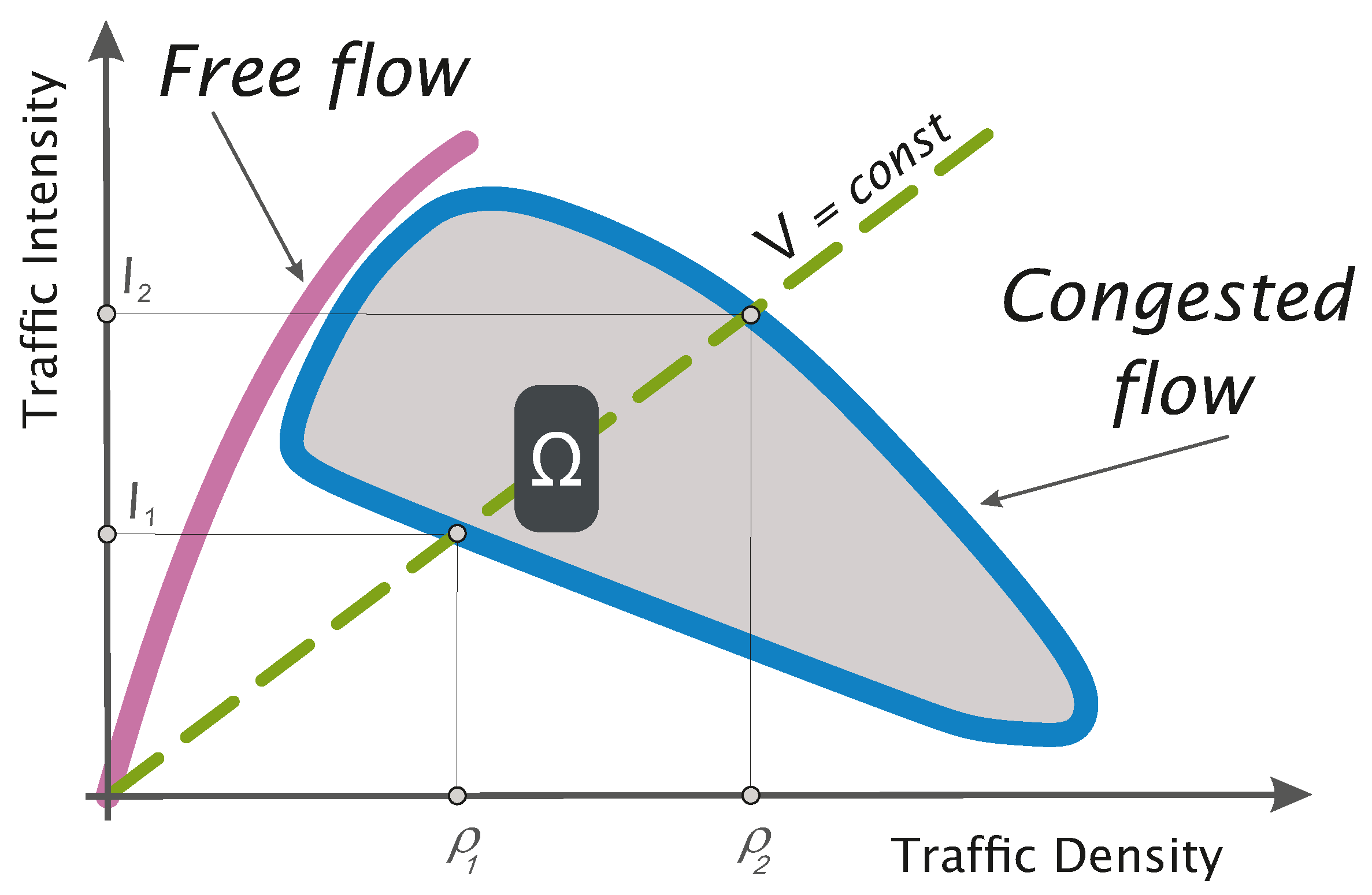
In this part of the text, we try to roughly summarize the current state of the art in the field of statistical analysis of traffic micro-quantities (quantities associated with individual vehicles, i.e., non-aggregated quantities). The physics of traffic ([4,15]) in the flow of time came to the conclusion that the statistics of traffic quantities are strongly sensitive to the current values of traffic macroscopic quantities (traffic density , traffic intensity I and average speed of the traffic sample V). And indeed, the mean values of the selected micro-quantities depend quite directly on the aforementioned macroscopic values, which is more or less trivial knowledge. A much more interesting finding is the fact that also the characteristics of higher orders (variance, typically) are strongly dependent on the location of the data sample in the so-called fundamental diagram, which is the two-dimensional graph of the binary relation between intensity and density (see [16]). A typical shape of such a graph is shown in Figure 1.

Figure 1.
Fundamental diagram of vehicular traffic—schematic representation of binary relation between traffic density and intensity extracted from typical empirical data samples. symbolizes a small sub-region with similar values of macroscopic quantities, where empirical data can be considered homogeneous.
It also soon became apparent that with a thoughtful way of analyzing empirical traffic data (when data extracted under different traffic conditions are not mixed), the hypothesis that vehicle speeds are normally distributed has been statistically confirmed several times (e.g., [17]). This means that the instantaneous speed of vehicles (with realization v) analyzed in a small sub-region (see Figure 1) is distributed with a probability density
which implies that the average value and the variance both of them depending on traffic density and intensity.
Much more interesting, however, are questions regarding the spatiotemporal arrangement of vehicles on roadways. Complex traffic dynamics (controlled by the decision-making processes in the driver’s brain) generate extremely interesting variants of the inner arrangement of a vehicular system. Surprisingly, some of them have no analogy to any of the classical physical systems. This is mainly due to a significant force repulsion, the main reason for which is the attempt to avoid a collision with other vehicles, predominantly with the preceding vehicle.
Common variants of the inner structure of a one-dimensional system can only be found in two special variants of the vehicular stream. The first of them is a situation where the traffic density is very low and therefore nothing forces the drivers to interact with each other. Such a situation, then (from a mathematical point of view), represents a so-called Poisson system, which is characterized by a total absence of interactions between elements of the system. In this type of system, the interval frequency (i.e., the number of particles occurring in an interval of fixed length L) follows the Poisson distribution
where stands for probability that in an interval of length L there is k elements/particles/vehicles. The mutual distances between neighboring particles in the Poisson system are then subject to the exponential distribution
where represents the Heaviside unit-step function. With regard to the above-mentioned properties, the Poisson system is understood as a system with the maximum possible freedom of movement, i.e., with the maximum degree of statistical fluctuations. Respective traffic states have been discussed in the earlier works [6,18].
A completely different version of a particle system is an ensemble with an absolutely perfect arrangement of elements, in which statistical fluctuations do not occur. It is a deterministic system, whose distribution of distances follows the Dirac distribution
which, in fact, describes equidistantly arranged one-dimensional ensembles (with mutual distance between neighbors equal to ). Generalized function is the Dirac delta impulse. The real vehicular system can approach the ideal Dirac system (see [19]), namely in a situation when the traffic density increases and mutual inter-vehicle interactions cause a transition into a highly correlated state, in which all vehicles move with approximately the same speed and headway, analogously to the motion of a solid block.
Apart from the two aforementioned marginal states, which can be described by textbook-types of distribution classes, in other cases, vehicles are grouped into statistically less expected constellations [6,20]. In some cases, the inner structure of vehicular samples even exceeds the limits that one-dimensional particle systems seem to have.
Although during the years when research in the field of VHM has been going on (and is still in progress), an overwhelming amount of different types of statistical description for the traffic micro-structure appeared, and over time it became clear that the relevant statistics must necessarily meet at least a minimum of theoretical or empirical assumptions. We speak about the criteria for admissibility. Let us briefly recall them here.
1.2. Criteria for Admissibility of Analytical Headway Statistics
The goal of this subsection is to mention certain universal attributes of vehicular headway statistics. Principally, regardless of the specific analytical form of the interaction forces/rules acting in the traffic flow, it is easy to see that their range is either short or medium. This refers to the fact that the group of vehicles that the driver takes into account in their decision-making process is either single-element or has only a few elements. Mathematically, such systems can be understood as quasi-Poisson systems. However, in quasi-Poisson systems, the statistic of distances between neighboring elements (probability density function) always belongs to the class of so-called balanced distributions (as proven in [21]). Balanced distributions are characterized by the fact that their asymptotic course is negatively exponential. To be specific,
For details regarding the class please see Appendix A.1.
Already in the early days of the physics of traffic (see Ref. [6] and references therein), the authors of various studies pointed out that the probabilities of short inter-vehicle distances are extremely low, or zero. The reasoning was straightforward, as follows. The effort not to cause a mutual collision forces the driver to maintain a certain safe distance from the bumper of the preceding vehicle, i.e., not allowing space clearances shorter than a certain critical value (clearance threshold), as claimed in initial research—e.g., [22]. Let us denote this threshold with the symbol So, drivers were actually forbidden from entering the critical area This led to the logical statement that the probability densities for clearances are shifted, i.e., they satisfy the equality Many studies then tried to detect this threshold (representing in fact the smallest measured gap between vehicles) from empirical data. And since the threshold detection task is very complex, the results showed quite contradictory values. The investigations confirmed the hypothesis that the greater the amount of measured data, the smaller the threshold. This hypothesis has been then confirmed several times, and in some studies (e.g., [6] and references therein), the detected threshold was barely distinguishable from zero. Mathematical extrapolation of these considerations leads to the following reasoning. If the amount of analyzed data grows to infinity, then the threshold tends toward zero. From here, it is only a step to finding out that the empirical distribution is indeed non-zero everywhere on but at the same time, drops enormously sharply (if ) to zero. This trend can be expressed mathematically (like in [7]) by the following definition
If the function meets this condition, we say that it has a plateau at the origin.
To conclude, theoretically acceptable headway distribution should have a plateau at the origin and belong to
2. Vehicular Spatiotemporal Micro-Quantities—Classification and Extraction from Empirical Data
Vehicular headways and their various alternatives represent key micro-quantities in traffic flow theory. They characterize how vehicles are positioned on the road or how they pass a given detector. Usually, they used to be defined less formally, like the time between two successive vehicles passing the same point on the same lane. However, here, we are trying to classify the vehicular micro-quantities more precisely and multifariously. A typical set of unaggregated traffic data obtained via magnetic induction double loops contains the following records:
- is the time instant when a front bumper of the kth car has intersected a detector line;
- is the time instant when a rear bumper of the kth car has intersected a detector line;
- represents the instantaneous speed of the kth vehicle;
- stands for the length of the kth vehicle;
Furthermore, additional data obtained by image processing methods are:
- is the position of the front bumper of the kth car at a fixed time;
- is the position of the rear bumper of the kth car at a fixed time;
With the help of these detector records, specific variants of spatiotemporal micro-quantities can then be defined as follows. Typically, the time headways/clearances are introduced by means of the respective relations
Analogously, spatial headways are then defined by
and spatial clearances (gaps) read
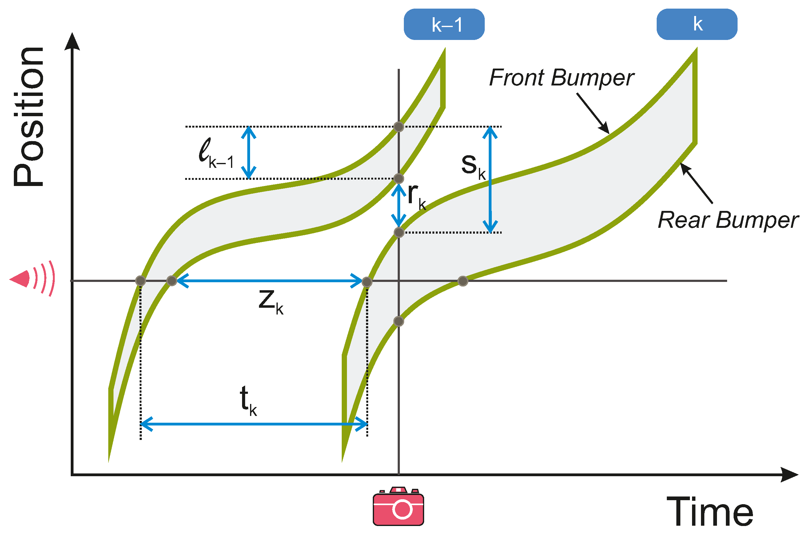
Graphically, all these quantities are visualized in Figure 2.
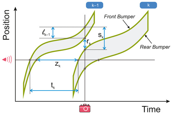
Figure 2.
Microscopic characteristics of traffic flow obtained with the help of a magnetic double-loop detector (time clearance and time headway ) or by image processing methods (space gap and space headway ).
From a mathematical point of view, all these micro-quantities represent, in fact, random variables, and therefore their analytical description should be mediated via corresponding statistical distributions (probability density functions or distribution functions). Their detection, prediction, and investigation of their temporal evolution is the cornerstone of the field of VHM.
3. Conversion of the Vehicular Stream to the Standard Physical System
The entire problem of kinematics and dynamics of the traffic system on a one-lane road can be quite naturally converted into the language of a classic one-dimensional system [15,20,23]. Once we exclude from our considerations the part of the road that is occupied by vehicles, i.e., if we reduce the vehicles to being dimensionless, then the traffic system can be viewed as a multi-particle system of mutually interacting elements, which is systematically disturbed by stochastic noise, the level of which is controlled by the coefficient of the so-called statistical resistivity. If its value is zero, the system is subjected to the maximum possible noise, which naturally leads to the highest fluctuations of the relevant descriptive characteristics. On the contrary, if ɛ increases beyond all limits, then the system becomes absolutely resistant to fluctuations and converges therefore to a deterministic system.
Mutual interactions in the system, which are of a two-body nature, can then naturally be described by a force dominated by repulsion preventing collisions [14,24]. In a system with a large number of particles—which is the case of vehicular traffic—it can then be assumed, without loss of generality, that forces between distant elements in the system are negligible. We are talking about a system with medium-ranged (or short-ranged) interactions, where the interaction is reduced to a few (or one) nearest neighbors only. Although in traffic models, dynamics description used to be introduced in a very complex manner (see for example Table 2.2 in [24]), it turns out that the most distinctive force factor is a strong repulsion from the rear bumper of the preceding car [24]. Usually, the relevant force is described by a relation
Effectively, this is a kind of analogy to the famous relationships of Isaac Newton and Charles-Augustin de Coulomb. In addition, some expert studies have shown that under certain circumstances, the traffic system can be credibly modeled by a thermodynamic gas (see explanation in Ref. [25], in which the law of action and reaction is fulfilled. In such a system, the force potential corresponding to the force description (10) is
Above that, the studies [23,26,27,28] have shown that in a homogeneous system of identical particles whose dynamics are driven by the same force description, spatial and time headway distributions can be derived from the potential Especially, in the case of short-ranged potentials, the probability density for the nearest neighbor distance is of the form
where and the constant assures the proper normalization.
Provided that the potential is strictly repulsive (like in Formula (11)), which means mathematically that
one can prove (see the diploma theses [29,30]) that holds, and
This implies that random variable —distributed via (12) with a strictly repulsive potential and scaled to unit average value—has always variance less than or equal to one. This is the key insight for the next part of the text.
We remark that for special choices of potentials , or we obtain the well-known exponential distribution (3), Gamma distribution
or two-parametric generalized inverse Gaussian distribution (GIG)
respectively. Here, stands for the Macdonald function of order Furthermore, the GIG density function (20) has—in contrast to the Gamma distribution (19)—a plateau at the origin, which is a great benefit.
4. Empirical Headway Distribution
Since the GIG distribution (20) meets both the empirical and theoretical criteria for admissibility, it can be therefore used in relevant procedures estimating headway distributions gauged on real freeways. Indeed, papers [11,12,23,31] show the successful applicability of such an approach. However, although the estimation procedure based on the GIG distribution is completely fruitful when applied to data measured on the main freeway lane, the fast lane data fail frequently. In the region of lower traffic densities, the deviations between the empirical course and the theoretical description are relatively large, as visualized in Figure 3.
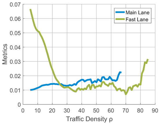
Figure 3.
We plot values of metrics measured between the histogram of empirical clearances and the theoretical prediction (20). Statistical estimations of parameters have been obtained by maximizing the statistical likelihood (MLE). The graphs clearly show a sharp decrease in the quality of the MLE estimates for the fast lane and traffic densities lower than 25 vehicles per kilometer. For the remaining cases, the quality of the estimates is basically constant.
This means that although the model settings used correspond well with the reality of traffic flow in the main lane, the same is not true for the vehicular stream in the fast lane. Moreover, it is clearly visible from Figure 3 that for densities more than 25 vehicles per kilometer the statistical estimates are equally plausible in both lanes. This is due to the fact that for higher traffic densities (when changing lanes does not bring any competitive advantage) both lanes are synchronized and their dynamics follow practically the same rules. Therefore, the inconsistency between the lanes is detected only if the overtaking maneuver provides some competitive advantage for sporty drivers.
5. Conversion to the Purely Mathematical Formalism
The kinematics of the described real problem can quite naturally be transferred to the world of random variables and their distributions. For these purposes, one of the suitable and highly effective instruments is the theory of balanced particle systems.
The motivation for introducing the particle systems is the rigorous description of one-dimensional systems of infinite length on which dimensionless particles (vehicles, pedestrians, agents) are stochastically distributed. The system follows the rule of simple exclusion, which means that two agents can not occupy the same location and, owing to the above-mentioned unidimensionality, they can be uniquely numbered. The reference agent is usually denoted by the index and numbering then proceeds chronologically. The entire system is understood as a stochastic system, i.e., the given state of the system is always described by probabilistic instruments. Although there are many ways by which a given system can be described statistically, the most common variants are the following sets of random variables.
- Random locations
- Random headways
- Random multi-headways
- Interval frequencies for any
The mathematical meaning of these quantities is clearly shown in Figure 4.
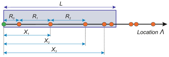
Figure 4.
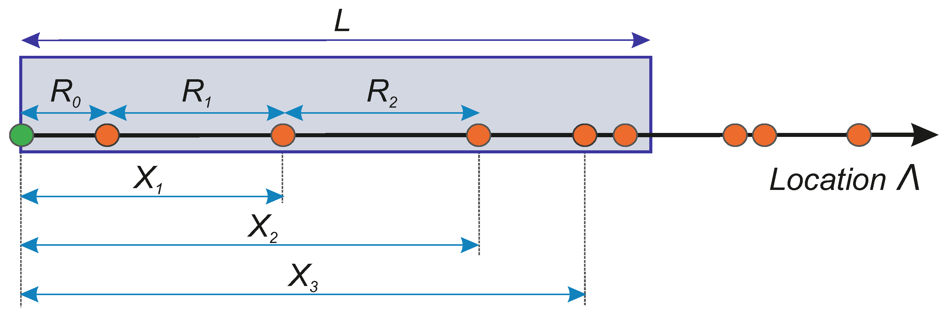
Graphical interpretation of initial random variables describing an arbitrary particle system. Green bullet represents the reference particle indexed by Other particles are visualized by orange bullets. Arrows represent mutual distances. Blue box of a length L symbolizes how the interval frequency is enumerated.
Random headways with realizations represent a distance between the agents indexed by k and Random multi-headways with realizations represent a distance between the reference agent and its kth neighbor. Interval frequency is understood as the number of agents occurring in the open interval The associate probabilistic inquiry reads and answers the question of what the probability is that exactly n agents lie in the interval.
Statistical description of headways/multi-headways is mediated by probability densities and respectively. A particle system is called balanced if all densities belong to the distribution class . If it is additionally assumed that the random variables are pairwise independent, then
holds, where ★ symbolizes a convolution. Since the class is alpha-stable, the result of the convolution belongs to class , i.e., The alpha stability brings many advantages in the corresponding analytical derivations.
For the purposes of modeling the traffic stream micro-structure, it can be assumed that the statistical distribution of gaps between succeeding cars is described by the same probability density. Under this circumstance, the common density is called the generator of the balance particle system.
In mathematical disciplines that deal with the issue of one-dimensional systems, a quantity called statistical rigidity plays a key role. According to [7,32,33,34], statistical rigidity is a continuous function describing the rate of fluctuations of the interval frequency and its dependence on the length of the interval Specifically:
The course of this function shows a marked linear asymptote, whose slope (statistical compressibility ) and intercept (statistical deflection ) reflects the intensity of mutual correlations between the agent’s locations. Above that, the theory of balanced particle systems has proven that the compressibility of systems with uncorrelated neighboring headways is equal to the variance of random variables , i.e.,
where is the kth momentum of all It means that for compressibility, one can read
Poissonian Particle System—Mathematical Attributes
As discussed earlier, a physical system is classified as Poissonian if the individual elements do not interact with each other in any way. Then—from a mathematical point of view—the occurrence of particles is of a purely random matter, and therefore, the interval frequency obeys the Poisson distribution (2). From here, it can be straightforwardly proven that the generator of such a system is an exponential function (3). Provided that we are concentrated on the scaled version of the system (as assumed in Equation (23)), then
and
Accordingly, for statistical rigidity of the Poissonian system, holds, which means that the Poissonian system has a compressibility equal to one.
If mutual interactions between agents are negligible, such a system quite naturally represents a certain boundary variant of a particle system. In other alternatives of particle systems where agents cooperate, mutual interaction suppresses the level of randomness, causing the rigidity to decrease (for a fixed value of L). Thus, while the compressibility of the Poisson system is equal to one, the compressibility of other systems is expected to be lower. We are talking about so-called sub-compressible systems (or states of one system).
6. Analysis of Compressibility for Empirical Traffic Samples
Vehicular traffic data samples analyzed in this paper have been gauged over 90 days at the two-lane freeway circuit D0 (located near Prague, Czech Republic) using induction double-loop detection technology. Statistical rigidity extracted from the empirical data samples (by applying the 3 s unification procedure explained in Ref. [14]) shows non-trivial dependence on traffic density and reveals fundamental differences between the two freeway lanes.
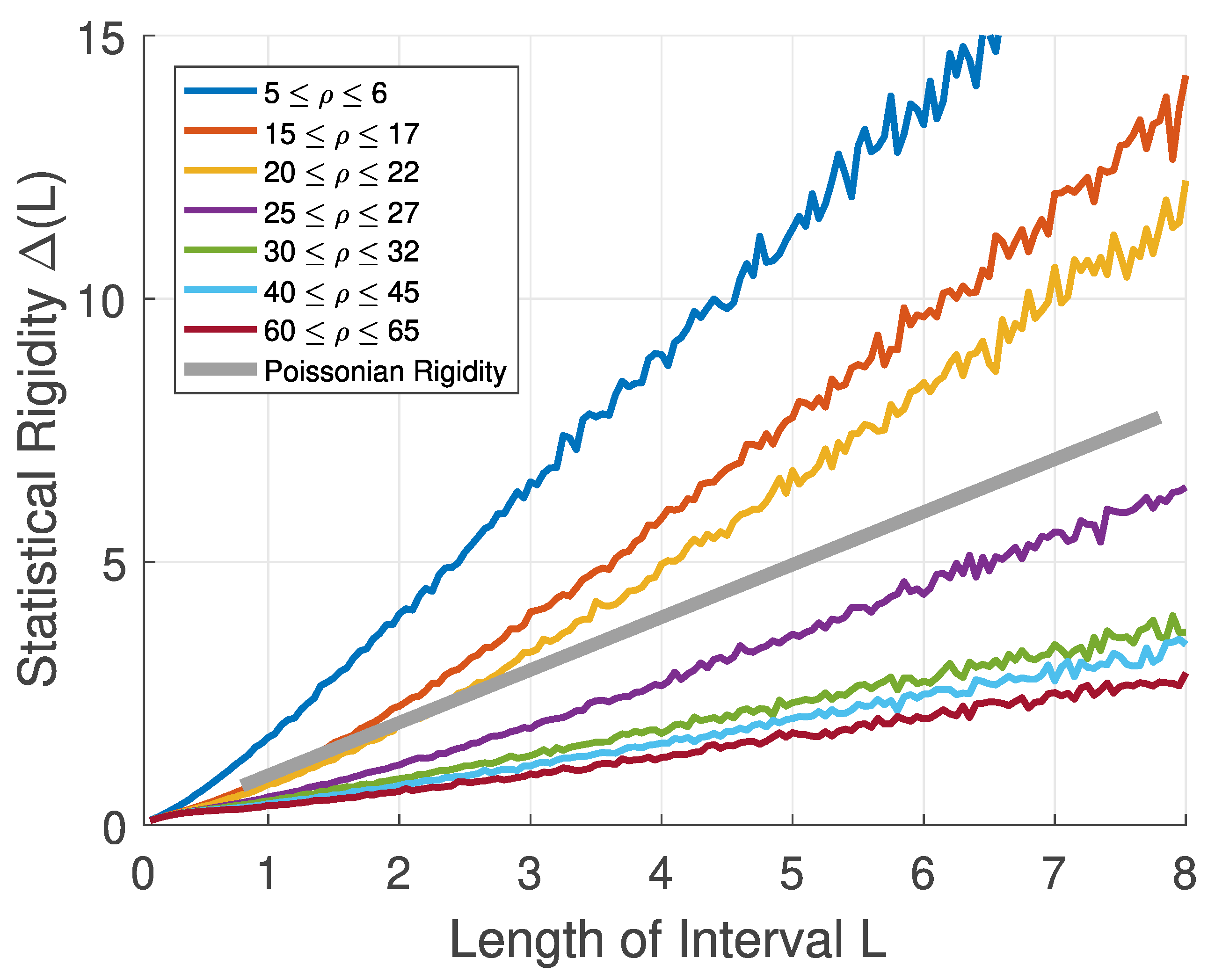
While the states of the traffic system recorded in the main lane are exclusively sub-compressible, in the fast lane, the same property is fulfilled only for higher values of traffic density (see Figure 5 and Figure 6). For traffic samples measured for the free phase of the fast-lane stream, the linear asymptote of statistical rigidity rises steeper than that calculated for Poisson systems. Its compressibility is therefore greater than one. Such states are called super-compressible. Note that the region of super-compressible states corresponds to regions where the statistical estimation procedures have been much less successful (see Figure 3). This coincidence, as will be seen later, is not accidental.
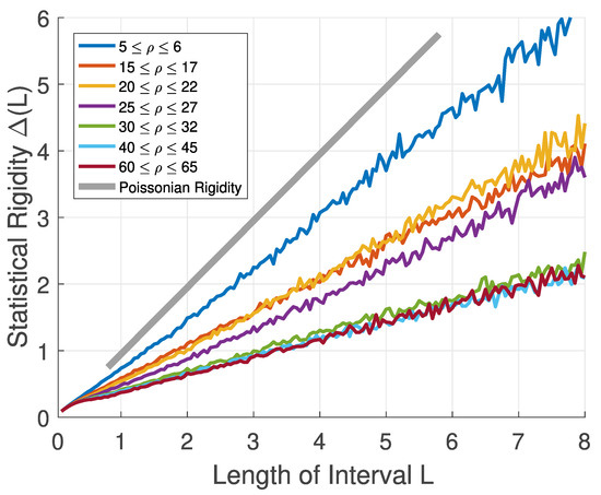
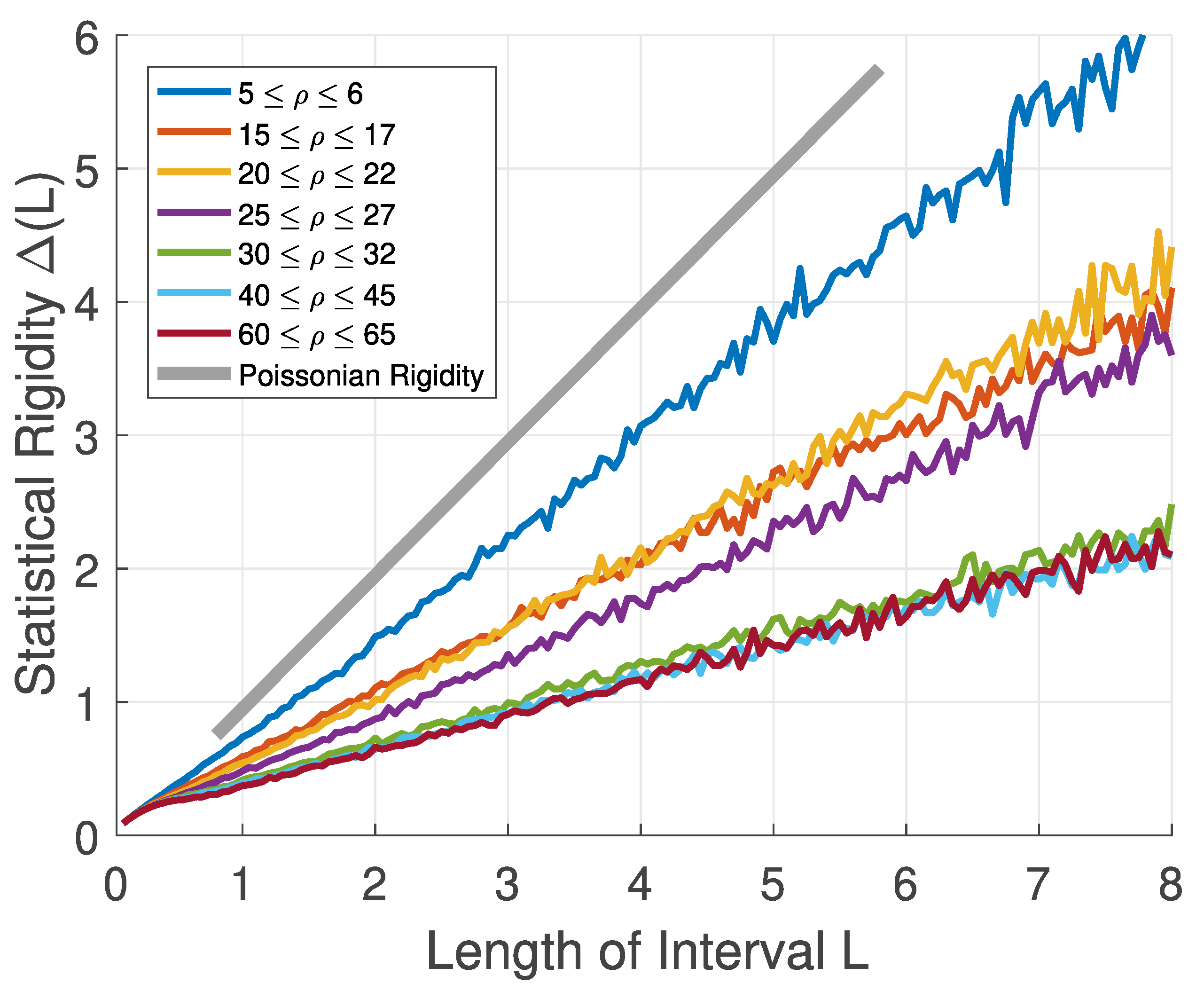
Figure 5.
We plot a graph of the statistical rigidity extracted from main-lane traffic data. Behavior of functions is visualized for traffic densities specified in the legend. For comparison purposes, we also plot the rigidity of the Poisson system. This figure was taken from Ref. [14]. Reproduced with permission from Krbálek et.al. Physica A, published by Elsevier 2022.

Figure 6.
We plot a graph of the statistical rigidity extracted from fast-lane traffic-data. Behavior of functions is visualized for traffic densities specified in the legend. For comparison purposes, we also plot the rigidity of the Poisson system. This figure was taken from Ref. [14]. Reproduced with permission from Krbálek et.al. Physica A, published by Elsevier 2022.
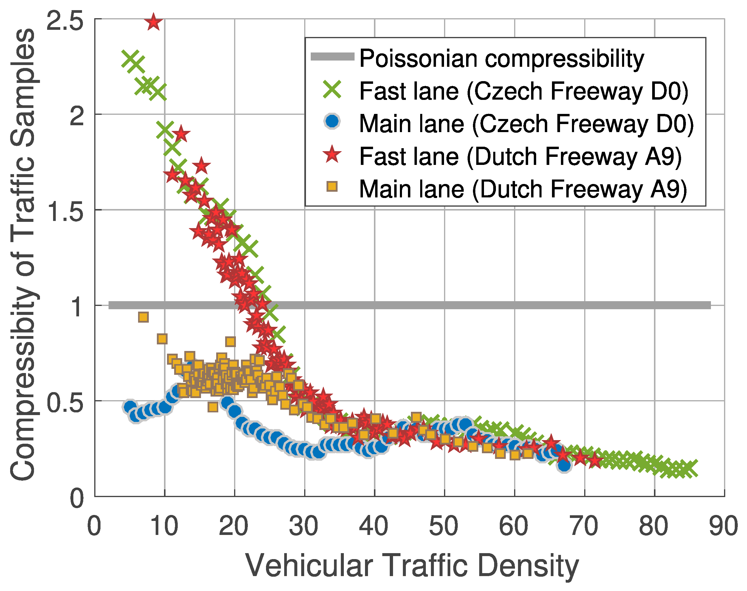
For clarity, we show in Figure 7 how the statistical compressibility changes depending on the traffic density. While most main-lane states are sub-compressible, at lower traffic densities in the fast lane, the compressibility exceeds the Poissonian border and the resulting states are therefore super-compressible. For robustness, we also mention here that super-compressible states have been recorded not only in freeway data samples but also in data measured inside cities. In Figure 8, it is confirmed that urban compressibility clearly follows the trend observed on European freeways.
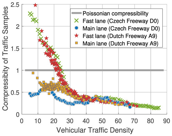
Figure 7.
The figure depicts the evolution of the statistical rigidity in different freeway lanes. This figure is replicated from the article [14]. Reproduced with permission from Krbálek et.al. Physica A, published by Elsevier 2022.

Figure 8.
The figure depicts the evolution of the statistical rigidity in main/fast lanes inside cities. Urban data were measured in the city of Vyškov in the Czech Republic.
To conclude, vehicular stream sometimes exhibits apparent illogicality, as it generates states in which the rate of fluctuations (here described by the tool of statistical rigidity) is significantly higher than is common for systems with absolute freedom of agent’s movement. And it is precisely these states that are estimated very imprecisely/unreliably even by the well-established estimation procedures. What is the real cause and what is the origin of these states?
7. Theoretical Derivations and Practical Consequences
In particle systems in which only the nearest neighbors interact (the so-called short-ranged interaction), it holds (as proved in the paper [23]) that the probability density for the distance between the succeeding particles has the form (12). If a purely repulsive potential (13)–(17) is chosen for such a system, then the following two findings result from the relation (18). If the analyzed clearances are scaled to a unit mean value, then their variance will never exceed the unit value. Furthemore, the statistical compressibility of such a system then acquires only values from the semi-closed interval (0, 1], whereas the unit value corresponds exclusively to the non-interaction variant of a system, i.e., the Poisson system. To summarize, it is proven analytically that all systems with short-ranged repulsive potential are sub-compressible or uni-compressible.
However, Figure 7 and Figure 8 show—beyond any doubt—that some constellations of traffic alignment are super-compressible. Three possible explanations follow from the aforementioned considerations:
- Under certain conditions, the vehicular flow represents a medium-ranged system, which means that the driver takes into account the behavior of several of his predecessors. This would violate the assumption of the short-ranged nature of inter-vehicular interactions.
- In standard traffic interactions, force repulsion is only a partial interaction factor. If the nature of the traffic flow allows it, drivers also use attractive control components. Particularly, these components are evident at lower traffic densities for more sporty drivers, who quite naturally line up in the fast freeway lane.
- Under certain conditions, the whole concept of the particle model fails because the basic assumption about the conservation of the number of particles in the system is violated. If the traffic density is lower, sporty drivers change lanes to a greater extent, which causes a significant deviation from the basic premise of the theoretical concept used.
But we can eliminate the first of the above justifications. Numerical analyses of particle systems show that an increase in the interaction range causes a decrease in the statistical rigidity values, which leads to lower compressibility values. Thus, by strengthening the interaction, the sub-compressible state cannot be flipped into the region of super-compressible states.
However, it is not possible to decide between the other two options based on theoretical considerations alone. This is well reasoned in [14], which admits both variants of the explanation. If it is not possible to decide theoretically, a suitable traffic experiment should be used to solve this open problem.
Super-Compressible Versions of Gig Distribution
By analytical means, it is quite easy to show that the two-parametric generalized inverse Gaussian distribution (GIG) of the form (20) is sub-Poissonian in all circumstances when This fully corresponds to the fact that the function (20) was created by substituting a purely repulsive potential into the general Formula (12).
If, instead of purely repulsive forces, we choose a dynamics that appropriately combines attractive and repulsive trends, the situation changes significantly. However, combining the two potentials must reflect the realistic nature of inter-vehicular interactions, i.e., for short clearances, the repulsion must significantly exceed the attractive force. Attraction, on the other hand, can manifest itself for long gaps between succeeding vehicles. Such requirements are met, for example, by the force description of the shape
This means that for a variant of homogeneous systems, one can write
For dynamics of this type, the resulting probability density is then a function
This function represents a rarely used version of the GIG distribution. This is a three-parameter family of distributions that can—provided that the parameters are appropriately set—exhibit variances greater than one. However, such a circumstance can only occur if . Then, if such a function plays the role of the generator in a particle system, this system is super-compressible.
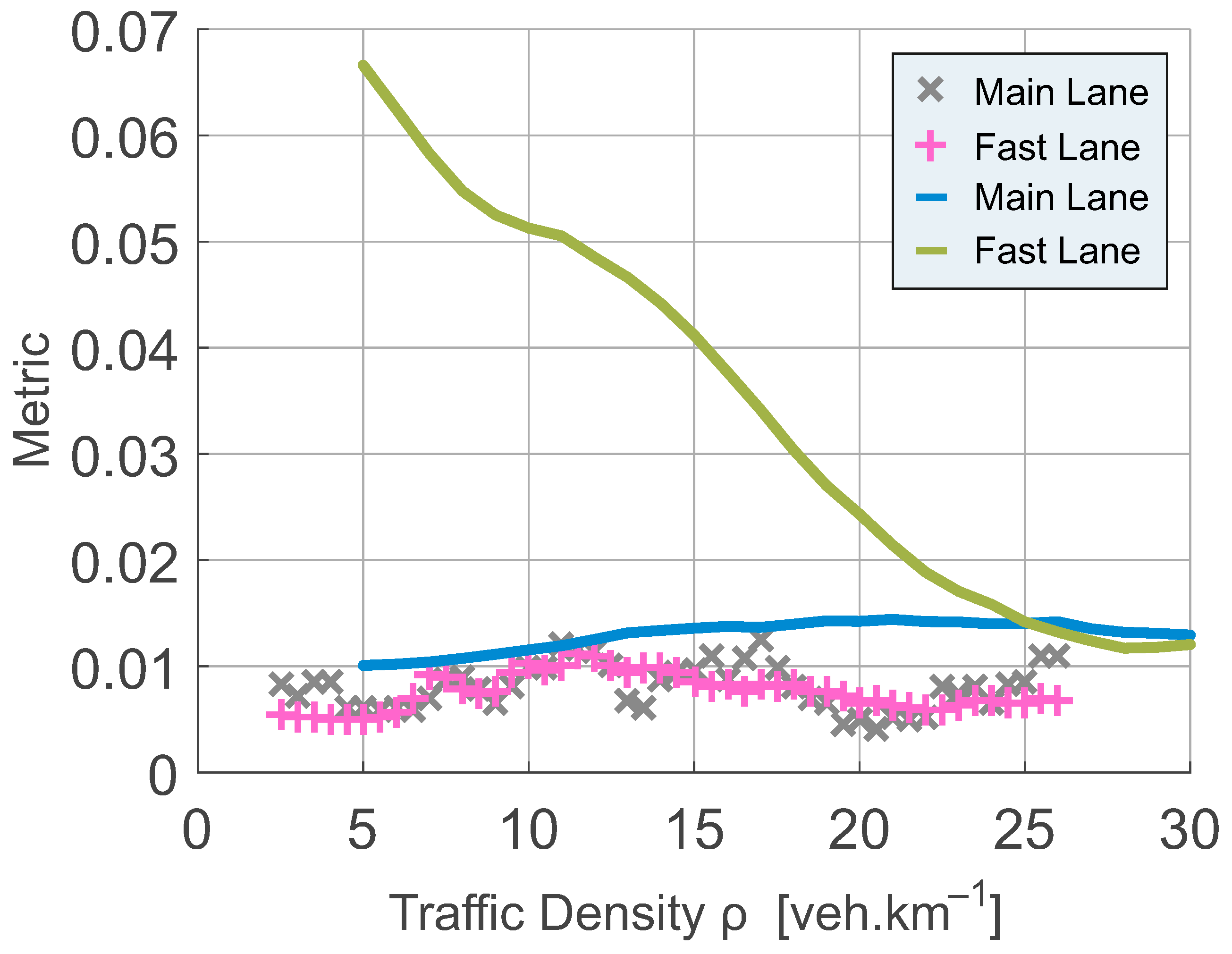
If we use the function (28) as the kernel in the MLE procedure estimating empirical clearance courses, such a procedure is significantly more successful than in the case cited in Section 4. Indeed, in Figure 9, we show not only that the presence of a third parameter increases the credibility of the estimation procedure (which is an expected consequence of the increase in the number of estimated parameters), but in particular, we point out that the metric measured between the optimal choice of the function and the empirical histogram shows no significant trend. Thus, the function replicates reliably even histograms that have been extracted from super-compressible traffic states. This implies that the presence of an attractive force component substantially improved the quality of the estimation. From the analysis of fitting results, it follows that attractive impulses are detected only in the fast lane and only if the competitive style of driving has a chance to be realized. Undoubtedly, this chance decreases with increasing traffic density when there is no room for sporting maneuvers.
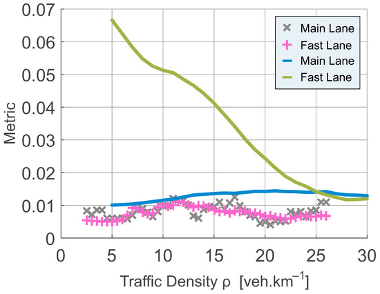
Figure 9.
Gray crosses and pink plus signs show the quality of the estimates that have been performed using three-parametric estimations that allow for the existence of super-compressible states. To highlight the quality of such estimates, we re-plot the original estimates (blue and green curves) based on the sub-compressibility assumption—see Figure 3.
8. Statistical Compressibility in Two Lanes Separated
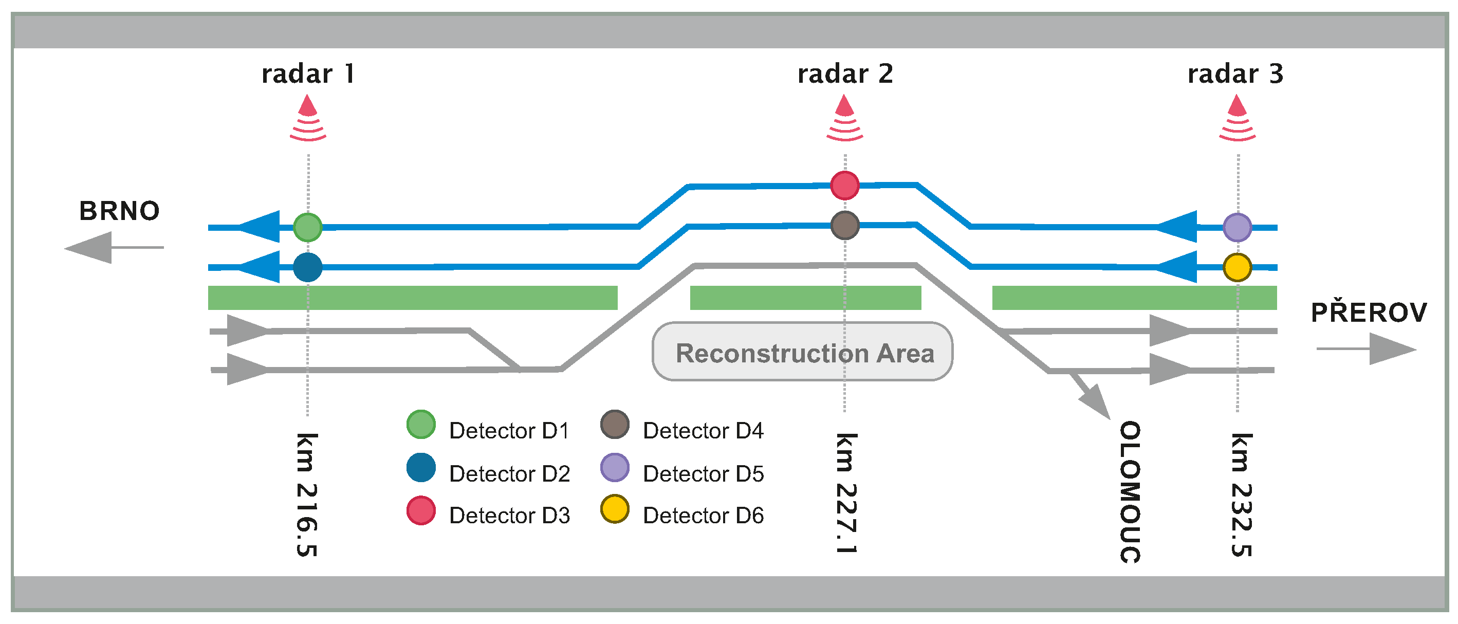
The data that we analyze in this section (2.35 mils events in total) were gauged during reconstruction works of Czech Expressway D1 (direction from Přerov to Brno) near city Vyškov during June, July, and August 2016, i.e., before COVID-19. The originally four-lane highway was narrowed and a barrier was installed between the fast and main lanes (in the direction toward Brno) to prevent vehicles from changing lanes. In the area of reconstruction, the maximum permitted speed was reduced to 80 km per hour. Here, three sets of radars (Wavetronics SmartSensor HD), having an accuracy: s for time measurements and 1 km/h for velocity measurements, have been located—as visualized in Figure 10. For purposes of measurements, a 16-kilometers-long segment near the reconstruction area has been chosen (see the Radar 2 in Figure 10). Detectors 3 and 4 represent an optimal choice for our intentions.
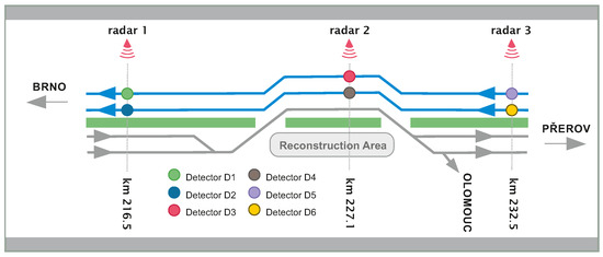
Figure 10.
Schematic representation of a freeway segment where the discussed traffic experiments were implemented.
Data required for the following statistical analyses have been processed with the help of the standard 3 s unification procedure. This means that only data from the same segment of the fundamental diagram (i.e., with similar values of traffic density and intensity) were evaluated together. Subsequently, data samples of inter-vehicular clearances have been re-scaled to a mean value equal to one. The data pre-processed by the above procedure have been then subjected to statistical estimations based on the minimum distance method (MDE). Specifically, we have used the metric
measuring the distance between empirical cumulative distribution functions and which are associated with the empirical histogram of clearances and density (28), respectively. The result of such statistical testing is the finding that the proposed three-parameter GIG model replicates the real courses of the histogram functions very convincingly and, moreover, relatively independently of the traffic density and the selected traffic lane. Thus, the distribution (28) represents a compact and robust tool for describing the traffic micro-structure of the traffic stream. But this is a relatively well-known fact (see [6,11,12,20,23]).
However, our main objective in this part of the text is to analyze the compressibility of vehicular traffic in reconstruction areas.
To be specific, we intend to use empirical data to decide
- Whether the safety precautions enforced by reconstruction constraints suppress the presence of super-compressible traffic states;
- Whether super-compressible states occur only in the fast lane as they do when there are no traffic restrictions;
- Whether, when the maximum speed of vehicles in the reconstruction area is sharply limited, the quantitative differences between the fast and slow lanes disappear.
For completeness, we add that samples containing trucks were excluded from the analysis. The presence of trucks would fundamentally change the behavior of the entire system, as understandable.
Subsequently, the interval frequency has been analyzed in the same segmentation way as the random variable in the previous part of the article. Significant emphasis has been put on the asymptotic behavior of statistical rigidity Individual values of rigidity enumerated for values L lying between 1 and 10—i.e., beyond the area of the curvilinear trend of rigidity—have been subjected to standard regression analysis. The slope of the obtained regression line is understood as an empirical value of the statistical compressibility of the traffic sample and is denoted by .
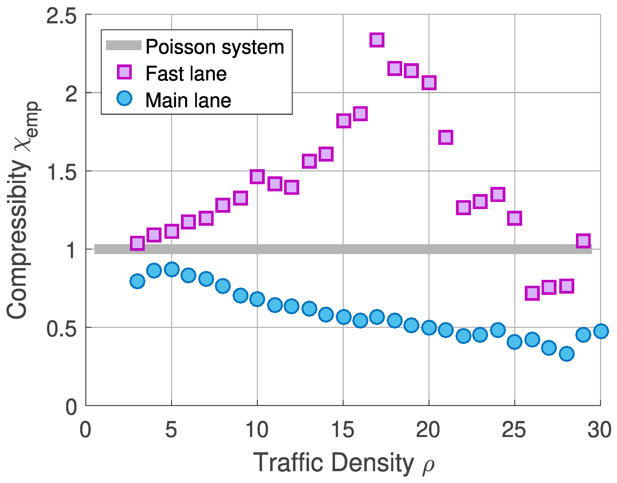
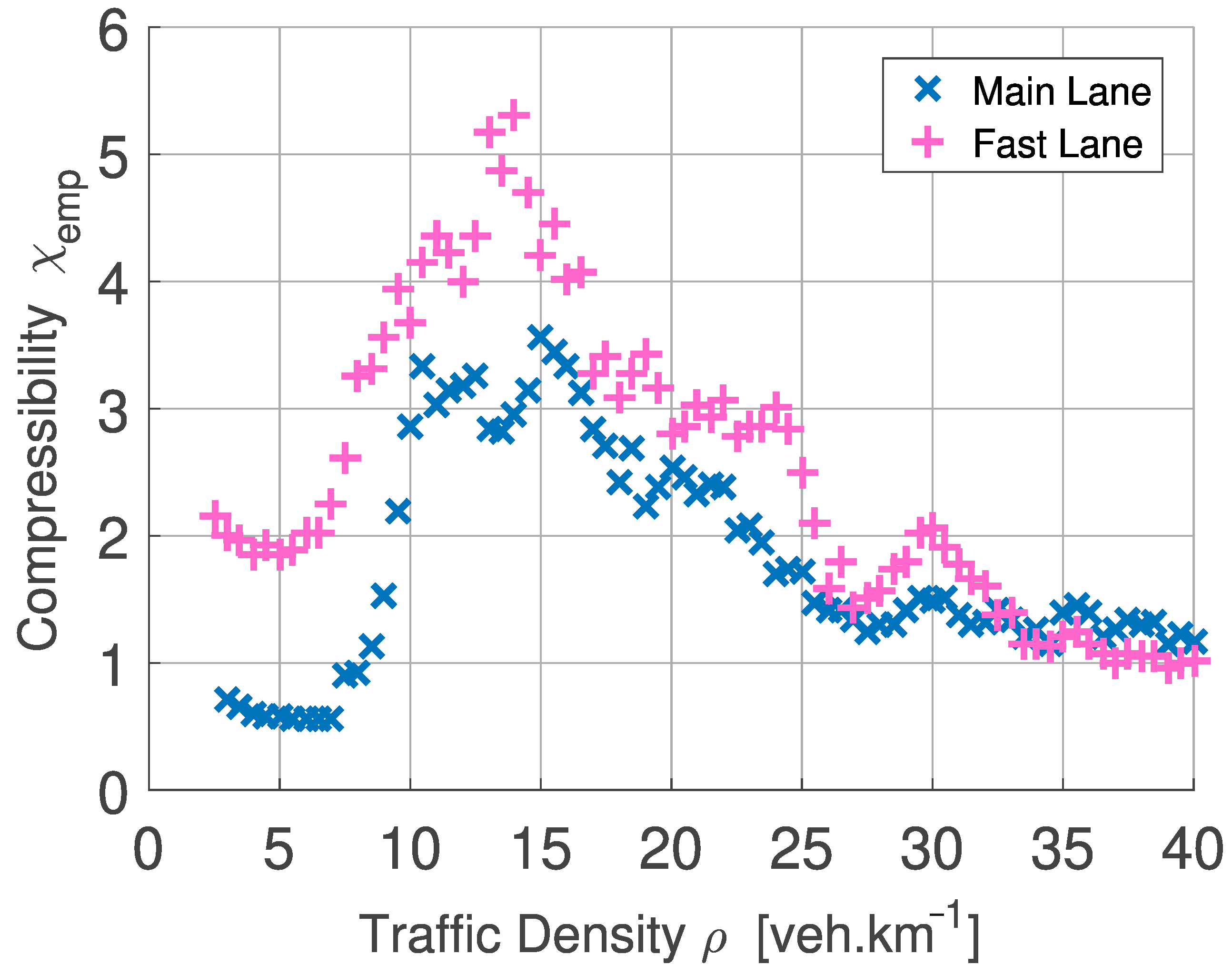
In Figure 11, one can spot the evolution of the statistical compressibility depending on traffic density in both lanes. The results of the analysis clearly show that even a physical barrier preventing vehicles from changing lanes did not erase the differences between the fast lane and the main lane. The substantial difference between the two compressibilities, which has been detected in previous research on two-lane freeways, is also clearly visible in the new data. And since these deviations can no longer be explained through the argument of increasing/decreasing the number of vehicles, this deviation must be a direct consequence of the different decision criteria of individual drivers in the two lanes. The second (rather surprising) finding is the fact that super-compressible states occur not only in the fast lane but also in the main lane. And since the super-compressible states indicate (in accordance with theoretical derivations) the presence of an attractive force component, it can now be argued that the interaction forces (which represent the physical transcript of the decision-making processes running in the driver’s brain) are mixed. This means that the repulsive force preventing collisions is also accompanied by an attractive force that corresponds to the driver’s effort to shorten the distance to the preceding vehicle. These findings are all the more surprising because the speed is limited to the same value in both lanes.
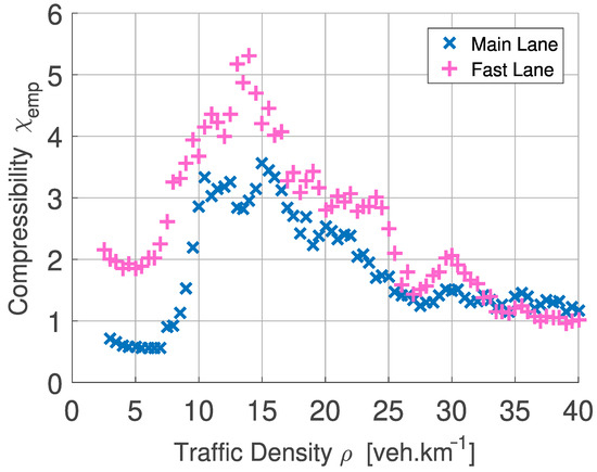
Figure 11.
Empirical values of statistical compressibility detected in traffic data measured in an area where traffic flow was significantly restricted due to reconstruction works. Data samples from the main (right) and fast (left) lanes were analyzed separately. Both lanes were separated by a barrier preventing lane−changing. The speed was limited to 80 km/h.
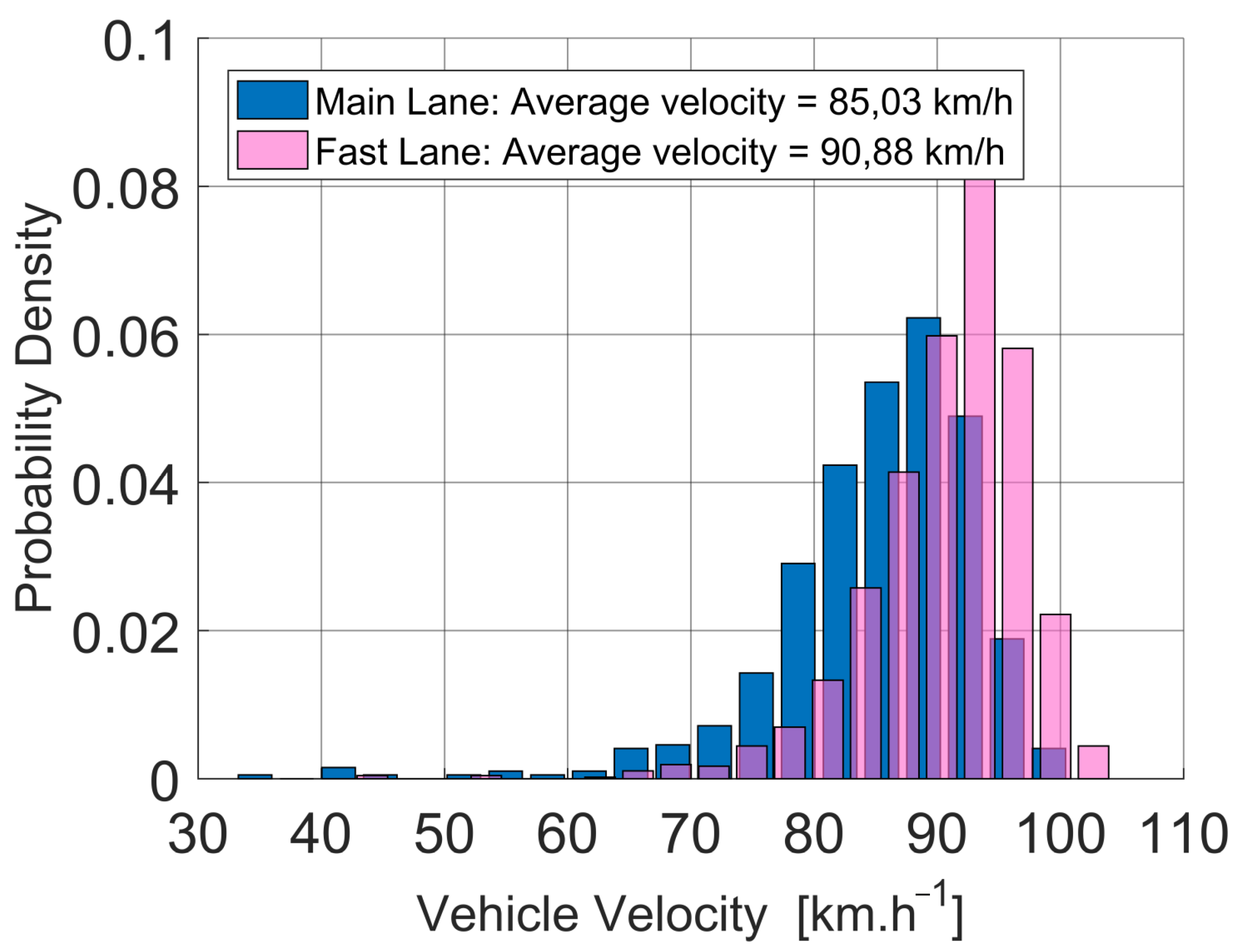
Thus, we find that although both traffic lanes are technically set to identical parameters, the driver’s brain does not choose the appropriate lane completely at random. On the contrary, drivers make spontaneous decisions based on their own driving style. It seems that more sporty drivers choose the fast lane to a greater extent, which is then reflected in an increased compressibility value. The consequence of this division is the fact that the statistical fluctuations of the traffic micro-quantities recorded in the fast lane are significantly more striking. The difference between the two lanes is also clearly visible in Figure 12, where a shift towards higher speeds is visible in the fast lane.
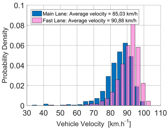
Figure 12.
Statistical distribution of vehicular speeds in individual traffic lanes. The velocities have been analyzed for traffic densities between 18 and 23 vehicles per kilometer.
9. Discussion and Conclusions
The article discusses atypical states in the micro-structure of the vehicular traffic system that seem to disrupt ingrained ideas about one-dimensional systems with maximum fluctuation rates. These states, which were found in empirical traffic data recorded at lower traffic densities, exceed the fluctuation rate of the Poisson systems, in which the freedom of particle movement is not restricted in any way, and which were intuitively suspected to be the upper limit for the fluctuation rate.
The experimentally detected anomalies were transformed by mathematical reformatting into the language of so-called balance particle systems. Within the framework of the relevant theory, the detected properties are much better quantified and the reasons for their occurrence are also more straightforwardly determined. In this way, it has been found that anomalous traffic states represent (from a mathematical point of view) so-called super-compressible states whose statistical compressibility (i.e., the slope of statistical rigidity) exceeds the unit value. By combining the physical background of the problem and the mathematical apparatus of balanced particle systems, it has been proven that super-compressible states in a closed system can occur only if an attractive force component acts between the particles of the system.
And since freeway flow analysis cannot rule out that the detected anomaly is caused by a large percentage of vehicles changing lanes during overtaking maneuvers, a traffic experiment was performed in which overtaking maneuvers were completely forbidden. For this purpose, the section of the freeway where the reconstruction work was taking place was chosen. The physical barrier between the narrowed lanes then served as an ideal overtaking blocker. The analysis of the measured data then convincingly revealed that super-compressible states occur even when the traffic streams are fully isolated.
To conclude, this study demonstrated that the repulsive force effect (which is a typical leading factor in all traffic models) is accompanied by a weaker inter-vehicular attraction, which has its origin in the competitive nature of sporty drivers. According to the results of this study, such an attractive force depends on the reciprocal value of the clearance, while the repulsive force depends on the reciprocal value of the square of the clearance. From a comparison of the mathematical nature of both dependencies, it is clear that for short clearances the repulsive impulses preventing collisions prevail, while for large clearances, the dominant component is the attractive force corresponding to the effort to catch up with the preceding vehicle.
However, it is important to note that this mixed nature of interactions can only be fully manifested for lower traffic density. Once the density reaches a threshold value (about 25 vehicles per kilometer), then the attractive component disappears and the flow in both streams becomes significantly synchronized.
To summarize, the added value of this article is the detection and explanation of anomalous traffic states that are quite common in all multi-lane traffic systems. As far as the authors of this article are aware, these states have never been relevantly investigated before. The presented research is based on relatively strong theoretical foundations, as it is based on a time-tested traffic model, which enables an analytical solution of the respective stationary states. In addition, the research is supported by a robust mathematical theory. As a current weak point of the research, we understand the limitation of the interpretation of the results to homogeneous traffic systems, i.e., systems composed only of passenger vehicles. The extension of the research to heterogeneous systems will be a logical continuation of the recent research.
Author Contributions
Methodology, M.K. (Milan Krbalek); numerical calculations, M.K. (Michaela Krbalkova); statistical analysis, M.K. (Michaela Krbalkova); validation, M.K. (Milan Krbalek) and M.K. (Michaela Krbalkova); investigation, M.K. (Milan Krbalek) and M.K. (Michaela Krbalkova); writing—original draft preparation, M.K. (Michaela Krbalkova); writing—review and editing, M.K. (Milan Krbalek); visualization, M.K. (Milan Krbalek) and M.K. (Michaela Krbalkova); supervision, M.K. (Milan Krbalek). All authors have read and agreed to the published version of the manuscript.
Funding
This research was funded by TAČR grant number CK01000152 and by the Ministry of Education, Youth, and Sports of the Czech Republic (MŠMT ČR) via grant SGS21/165/OHK4/3T/14.
Institutional Review Board Statement
Not applicable.
Informed Consent Statement
Not applicable.
Data Availability Statement
Research data analyzed in this paper are subject to a publication embargo. The data provider reserves the right not to provide the data to third parties.
Acknowledgments
We would like to thank The Road and Motorway Directorate of the Czech Republic for providing vehicular data discussed in our article.
Conflicts of Interest
The authors declare no conflicts of interest. The funders had no role in the design of the study; in the collection, analyses, or interpretation of data; in the writing of the manuscript; or in the decision to publish the results.
Abbreviations and Symbols
The following abbreviations/symbols are used in this manuscript:
| VHM | Vehicular headway modeling |
| E | Expectation of random variable |
| D | Statistical variance |
| ★ | Functional convolution |
| Probability of event A | |
| Set of natural number | |
| Set of real number | |
| Class of balanced densities | |
| Heaviside unit-step function | |
| Random variables with realisations z | |
| k–th Momentum of random variable | |
| Random locations | |
| Inter-vehicular headways with realisations | |
| Inter-vehicular multi-headways with realisations | |
| Interval frequency with parameter | |
| Macdonald’s function of order a | |
| Interaction force | |
| Interaction potential | |
| Statistical rigidity | |
| Statistical compressibility | |
| Time headway | |
| Time clearance | |
| Space headway | |
| Space clearance (gap) | |
| Vehicle velocity |
Appendix A
Appendix A.1. Class of Balanced Densities
A function is called a balanced density (balanced density function) if fulfilling the following axioms:
- Piece-wise continuity: , i.e., is piece-wise continuous on
- Non-negativity of the range: , i.e., is non-negative;
- Non-negativity of the support: , i.e., ;
- Lebesgue integrability: , i.e., is Lebesgue integrable;
- Balancing tail: so thatand
The parameter is called a balancing index. The class of balanced densities is denoted by The balanced density will be referred to as the normalized (balanced) density if Therefore, every normalized density can be understood as the probability density function of a certain continuous random variable. Moreover, according the balancing criterion, density function is balanced (with the balancing index equal to ) if and only if
Representatives of the set are, for example, exponential distribution, Erlang distribution, Gamma distribution, inverse Gaussian distribution, and generalized inverse Gaussian distribution. Contrarily, log-normal distribution or normal distribution does not belong to
Appendix A.2. Point Scenario of the Research
In this section, we summarize all the basic steps that were carried out within the presented research.
- Statistical analysis of inter-vehicle clearances gauged on Dutch and Czech freeways. The collection of data samples would be carried out before the outbreak of the COVID-19 epidemic.
- Detection of anomalous areas of the fundamental diagram.
- Analysis of the statistical rigidity and compressibility. Delimitation of the areas of super-compressible states.
- Linking the thermodynamic traffic model with the theory of balance particle systems.
- A mathematical proof of the key theorem of this paper. This theorem proves that in systems with a pure inter-particle repulsion, the compressibility is always less than or equal to one.
- Formulation of three admissible justifications for the existence of super-compressible states in the traffic micro-structure.
- Elimination of one of these three justifications by means of numerical simulations of the thermodynamic traffic model [23].
- Design and implementation of a traffic experiment, with the help of which it is possible to decide which of the two remaining effects causes the supercompressibility of traffic data.
- Evaluation of traffic-flow data gauged in a region of reconstruction work.
- Determination of the definitive justification for the existence of anomalous traffic states.
- Interpretation of the findings in the terminology of the driver’s decision-making process.
References
- Nagel, K.; Schreckenberg, M. A cellular automaton model for freeway traffic. J. Phys. Fr. 1992, 2, 2221. [Google Scholar] [CrossRef]
- Fukui, M.; Ishibashi, Y. Traffic flow in 1D cellular automaton model including cars moving with high speed. J. Phys. Soc. Jpn. 1992, 65, 1868. [Google Scholar] [CrossRef]
- Derrida, B.; Domany, E.; Mukamel, D. An exact solution of a one-dimensional asymmetric exclusion model with open boundaries. J. Stat. Phys. 1992, 69, 667. [Google Scholar] [CrossRef]
- Treiber, M.; Kesting, A. Traffic Flow Dynamics; Springer: Berlin/Heidelberg, Germany, 2013. [Google Scholar]
- Kerner, B.S. The Physics of Traffic; Springer: New York, NY, USA, 2004. [Google Scholar]
- Li, L.; Chen, X.M. Vehicle headway modeling and its inferences in macroscopic/microscopic traffic flow theory: A survey. Transp. Res. Part 2017, 76, 170. [Google Scholar] [CrossRef]
- Kollert, O.; Krbálek, M.; Hobza, T.; Krbálková, M. Statistical rigidity of vehicular streams—Theory versus reality. J. Phys. Commun. 2019, 3, 035020. [Google Scholar] [CrossRef]
- Krbálek, M.; Hobza, T. Inner structure of vehicular ensembles and random matrix theory. Phys. Lett. 2016, 380, 1839. [Google Scholar] [CrossRef]
- Abul-Magd, A.Y. Modeling highway-traffic headway distributions using superstatistics. Phys. Rev. E 2007, 76, 057. [Google Scholar] [CrossRef]
- Chen, X.; Li, L. A Markov Model for Headway/Spacing Distribution of Road Traffic. IEEE Trans. Intell. Transp. Syst. 2010, 11, 773. [Google Scholar] [CrossRef]
- Roy, R.; Saha, P. Headway distribution models of two-lane roads under mixed traffic conditions: A case study from India. Eur. Transp. Res. Rev. 2018, 10, 3. [Google Scholar] [CrossRef]
- Bari, C.S.; Chandra, S.; Dhamaniya, A. Service headway distribution analysis of FASTag lanes under mixed traffic conditions. Physica A 2022, 604, 127904. [Google Scholar] [CrossRef]
- Gartzke, S.; Wang, S.; Guhr, T.; Schreckenberg, M. Spatial correlation analysis of traffic flow on parallel motorways in Germany. Physica A 2022, 599, 127367. [Google Scholar] [CrossRef]
- Krbálek, M.; Šeba, F.; Krbálková, M. Super-random states in vehicular traffic—Detection & explanation. Physica A 2022, 585, 126418. [Google Scholar]
- Helbing, D. Traffic and related self-driven many-particle systems. Rev. Mod. Phys. 2001, 73, 1067. [Google Scholar] [CrossRef]
- Wikipedia. Available online: https://en.wikipedia.org/wiki/Relation_(mathematics) (accessed on 14 August 2023).
- Helbing, D. Fundamentals of traffic flow. Phys. Rev. E 1977, 55, 3735. [Google Scholar] [CrossRef]
- Cowan, R.J. Useful Headway Models. Transp. Res. 1975, 9, 371. [Google Scholar] [CrossRef]
- Helbing, D.; Huberman, B.A. Coherent moving states in highway traffic. Nature 1998, 396, 738. [Google Scholar] [CrossRef]
- Li, L.; Jiang, R.; He, Z.; Chen, X.M.; Zhou, X. Trajectory data-based traffic flow studies: A revisit. Transp. Res. Part Emerg. Technol. 2020, 114, 225. [Google Scholar] [CrossRef]
- Krbálek, M.; Hrabák, P.; Bukáček, M. Pedestrian headways—Reflection of territorial social forces. Physica A 2018, 490, 38. [Google Scholar] [CrossRef]
- Greenberg, I. The log-normal distribution of headways. Austral. Road Res. 1966, 2, 14. [Google Scholar]
- Krbálek, M. Equilibrium distributions in thermodynamical traffic gas. J. Phys. A Math. Theor. 2007, 40, 5813. [Google Scholar] [CrossRef]
- Chen, X.M.; Li, L.; Shi, Q. Stochastic Evolutions of Dynamic Traffic Flow: Modelling and Application. In Traffic Flow Dynamics; Springer: Berlin/Heidelberg, Germany, 2014. [Google Scholar]
- Treiber, M.; Helbing, D. Hamilton-like statistics in one-dimensional driven dissipative many-particle systems. Eur. Phys. J. B 2009, 68, 607. [Google Scholar] [CrossRef]
- Bogomolny, E.B.; Gerlland, U.; Schmit, C. Short-range plasma model for intermediate spectral statistics. Eur. Phys. J. B 2009, 19, 121. [Google Scholar] [CrossRef]
- Scharf, B.; Izrailev, F.M. Dyson’s Coulomb gas on a circle and intermediate eigenvalue statistics. J. Phys. A Math. Gen. 1990, 23, 963. [Google Scholar] [CrossRef]
- Helbing, D.; Treiber, M.; Kesting, A. Understanding interarrival and interdeparture time statistics from interactions in queuing systems. Physica A 2006, 363, 62. [Google Scholar] [CrossRef]
- Lhotaková, A. Scaling and Estimating for GIG-Distributed Data. Master’s Thesis, Czech Technical University, Prague, Czech Republic, 5 January 2023. [Google Scholar]
- Pánek, V. Statistical Properties of Thermodynamic Particle Gas with Combined Potential. Master’s Thesis, Czech Technical University, Prague, Czech Republic, 2 May 2022. [Google Scholar]
- Wu, S.; Zou, Y.; Wu, L.; Zhang, Y. Application of Bayesian model averaging for modeling time headway distribution. Physica A 2023, 620, 128747. [Google Scholar] [CrossRef]
- Mehta, M.L. Random Matrices, 3rd ed.; Academic Press: New York, NY, USA, 2004. [Google Scholar]
- Chalker, J.T.; Kravtsov, V.E.; Lerner, I.V. Spectral Rigidity and Eigenfunction Correlations at the Anderson Transition. J. Exp. Theor. Phys. Lett. 1996, 64, 386. [Google Scholar] [CrossRef]
- Bohigas, O. Random Matrix Theories and Chaotic Dynamics; Elsevier Science Publisher: Paris, France, 1991. [Google Scholar]

Disclaimer/Publisher’s Note: The statements, opinions and data contained in all publications are solely those of the individual author(s) and contributor(s) and not of MDPI and/or the editor(s). MDPI and/or the editor(s) disclaim responsibility for any injury to people or property resulting from any ideas, methods, instructions or products referred to in the content. |
© 2024 by the authors. Licensee MDPI, Basel, Switzerland. This article is an open access article distributed under the terms and conditions of the Creative Commons Attribution (CC BY) license (https://creativecommons.org/licenses/by/4.0/).