Historical Elite Differential Evolution Based on Particle Swarm Optimization Algorithm for Texture Optimization with Application in Particle Physics

Abstract

Within the phenomenology of particle physics, the theoretical model of 4-zero textures is validated using a chi-square criterion that compares experimental data with the computational results of the model. Traditionally, analytical methods that often imply simplifications, combined with computational analysis, have been used to validate texture models. In this paper, we propose a new meta-heuristic variant of the differential evolution algorithm that incorporates aspects of the particle swarm optimization algorithm called “HE-DEPSO” to obtain chi-squared values that are less than a bound value, which exhaustive and traditional algorithms cannot obtain. The results show that the proposed algorithm can optimize the chi-square function according to the required criteria. We compare simulated data with experimental data in the allowed search region, thereby validating the 4-zero texture model.

1. Introduction

Broadly speaking, physics can be classified into three areas: the theoretical part, which, through mathematical formalism, explains and understands the physical phenomena; the experimental part, which groups disciplines related to the acquisition of data, the methods of data acquisition, and the design and performance of experiments; and finally, the aspect that links these two, known as phenomenology, which deals with (1) validating theoretical models, (2) investigating how to measure their parameters, (3) investigating how to distinguish one model from another, and (4) studying the experimental consequences of these models. This paper addresses a phenomenological approach by providing a solution to the validation of a theoretical model of physics, more specifically, from particle physics, to unveil the mechanisms of fermion mass generation and to reproduce the elements of the $V_{CKM}$ (Cabibbo–Kobayashi–Maskawa unitary matrix), which describes the mixing of different types of quark during weak interactions by encapsulating the probabilities of transitions between these quark types (see, for example, pertinent introductory reviews [1,2,3]), known as the mixing matrix.

The beginning of these models goes back to the first years of the 1970s, shortly after the establishment of the standard model (SM) of particle physics. Since then, different approaches have been developed in the context of theoretical and phenomenological models, which can be broadly classified as follows: Radiative mechanisms, where fermion masses come from contributions of processes generated by new particles added to SM [4,5]; Textures, where the mass matrix has zeros in some entries [6,7,8]; Symmetries between families, where a mathematical group symmetry is added to the theory [9,10]; and Seesaw mechanisms, an elegant way of generating small masses for neutrinos [11,12,13]. These approaches are phenomenological interrelated; for example, when we add an extra group symmetry to the theory it is common to arrive at texture structure to mass matrices [14,15], and in linear and inverse Seesaw models a texture structure is used to obtain the neutrino masses [16].

The texture formalism was born by considering that certain entries of the mass matrix are zero, such that we can compute analytically the matrix that diagonalizes it and hence the matrix $V_{CKM}$. In 1977, Harald Fritzsch created this formalism by using 6-zero hermetic textures as a viable model [17]; in 2005, with experimental data from that year, he found that 4-zero hermetic textures were viable to generate the quark masses and the mixing matrix [18]. The analytical approach is very complex, so certain considerations are made to simplify the model. However, the results obtained are not accurate, which is why numerical approaches have recently been used to obtain more accurate solutions. Given the precision of the current experimental data, it is worthwhile assessing the feasibility of these texture models with early studies on the 4-zero mass matrix [19], further exploring their potential to align with experimental data.

There are numerical works on 4-zero texture models; however, the detailed numerical descriptions of the techniques and algorithms used are not described by their authors [20]. The numerical analysis of texture models requires a ${\chi }^2$ criterion that establishes when the theoretical part of the model agrees with the experimental part [21]. That is, to validate the model, a function (which we will call ${\chi }^2\left(X\right)$) is built, and permissible values of the free parameters X of the model must be found, such that this function takes the minimum value possible greater than 0 but less than 1. In other words, it is necessary to optimize said function under a certain threshold. For the particular case of the function ${\chi }^2\left(X\right)$ obtained from the texture formalism, the difficulty comes from the cumbersome algebraic manipulation of the expressions involved, which complicate and entangle the application of classic optimization techniques; thus, alternative optimization techniques are required.

To the best of the authors’ knowledge, the works where bio-inspired optimization algorithms have been used within particle physics are as follows: in experimental contexts, where particle swarm optimization algorithms (PSOs), as well as genetic algorithms (GAs), have been implemented within the hyperparameter optimization of machine-learning (ML) models used in the analysis of data obtained in high-energy physics experiments [22]; in the optimization of the design of particle accelerators, where the differential evolution (DE) algorithm is quite effective [23,24]; and in phenomenology, where genetic algorithms have been used to discriminate models from supersymmetric theories [25].

As can be seen, the incursion of bio-inspired optimization algorithms in particle physics has been very limited, even when the results are favorable. For this reason, further application of these techniques and algorithms in this type of particle physics area, especially in texture formalism, is of great interest.

The DE algorithm is one of the evolutionary algorithms that has stood out the most in recent times due to its simplicity, power, and efficiency [26,27]; however, like other evolutionary algorithms, it is likely to suffer premature convergence and stagnation in local minima [26,28]. The strategies implemented to solve these problems can be classified as follows [29]:

• Change the mutation strategy. The mutation phase of the DE algorithm is important since it allows the integration of new individuals into the existing population, thus influencing its performance. Algorithms such as CoDE [30] have introduced new mutation strategies and implemented different mutation strategies, respectively, in order to improve the efficiency of the DE algorithm.
• Change the parameter control. The DE algorithm is sensitive to the configuration of its main parameters: the scale factor F and the crossover probability $Cr$ [26,31]. Self-adaptive control of these parameters has been shown to improve the performance of the DE algorithm significantly. In this sense, the SHADE [32] and SaDE [33] algorithms represent two fairly well-known variants.
• Incorporation of population mechanisms. The way in which the population is handled in the DE algorithm can improve its performance. Techniques such as genotypic topology [34], opposition-based initialization [35], and external population archives, as seen in JADE [36], have shown positive effects.
• Hybridization with other optimization algorithms. One way to improve the performance of the DE algorithm is to take advantage of the operators’ strengths from other algorithms and incorporate them into the structure of the DE algorithm through a hybridization process [27,37]. Hybridization with other computational intelligence algorithms, such as artificial neural networks (ANNs), ant colony optimization (ACO), and particle swarm optimization (PSO), has marked a trend within the last decade [27,38].

The self-adaptive differential evolution algorithm based on particle swarm optimization (DEPSO) [39] is a recent variant of the DE algorithm that integrates the PSO mutation strategy within its structure. DEPSO employs a probabilistic selection technique to choose between two mutation strategies: a new mutation strategy with an elite file called DE/e-rand/1, a modification of the DE/rand/1 strategy, and the mutation strategy of the PSO algorithm. This probabilistic selection technique enables DEPSO to improve the balance between exploitation and exploration, resulting in significantly better performance compared to both DE and PSO on various single-objective optimization problems.

This paper proposes a new variant of the DEPSO algorithm called historical elite differential evolution based on particle swarm optimization (HE-DEPSO) to improve optimization performance in solving complex single-objective problems, with a specific focus on addressing the problem of optimizing the ${\chi }^2$ criteria for the 4-zero texture model of high energy physics. The proposed variant aims to explore the areas of opportunity encountered to enhance DEPSO, specifically introducing a new mutation strategy named DE/current-to-EHE/1, which utilizes information from the elite individuals of the population and incorporates historical data from the evolutionary process to improve the balance between exploration and exploitation by leveraging information from elite individuals and historical data, particularly during the early stages of the evolutionary process. Additionally, HE-DEPSO employs the self-adaptive parameter control mechanism from the SHADE algorithm to reduce the sensitivity of the algorithm’s parameters. To test the HE-DEPSO algorithm’s performance, it was compared against other optimization algorithms, including DE, PSO, CoDE, SHADE, and DEPSO, using the CEC 2017 single-objective benchmark function set. The HE-DEPSO algorithm outperformed the other algorithms in terms of solution quality. Finally, the validation of the 4-zero texture model was conducted, optimizing the ${\chi }^2$ function and, at the same time, comparing the performance of our proposal against DE, PSO, CoDE, SHADE, and DEPSO algorithms for this particular application. The results are encouraging and expand the use of bio-inspired methods in high-energy physics by integrating a metaheuristic approach.

The remainder of the paper is structured as follows: Section 2 contains the definition of the problem to be solved, including the definition of the ${\chi }^2$ criterion; Section 3 reviews the versions of the PSO and DEPSO algorithms used here. Section 4 explains our proposal, the HE-DEPSO algorithm; Section 5 subjects our algorithm to benchmark tests, while Section 6 presents the validation problem of the 4-zero texture model. Finally, in Section 7, the conclusions are presented.

2. Problem Definition

Within the scope of the SM, the masses of the quarks come from hermetic $3\times 3$ matrices known as mass matrices (one for u-type quarks and another for d-type quarks) [40,41,42], as the absolute values of their eigenvalues and the matrix $V_{CKM}$ as the product of the matrix that diagonalizes the u-type quarks and the matrix that diagonalizes the d-type quarks; however, due to the mathematical formalism used, the mass matrices remain entirely unknown and, consequently, the masses of the quarks and the mixing matrix $V_{CKM}$ cannot be theoretically predicted. The experiment provides us with the numerical value of these quantities.

The mixing matrix $V_{CKM}$ can be written in a general way as:

$$V_{CKM}=\left(\begin{array}{ccc}{\left(V_{CKM}\right)}_{ud}& {\left(V_{CKM}\right)}_{us}& {\left(V_{CKM}\right)}_{ub}\\ {\left(V_{CKM}\right)}_{cd}& {\left(V_{CKM}\right)}_{cs}& {\left(V_{CKM}\right)}_{cb}\\ {\left(V_{CKM}\right)}_{td}& {\left(V_{CKM}\right)}_{ts}& {\left(V_{CKM}\right)}_{tb}\end{array}\right)$$

(1)

and is a unitary matrix containing information about the probability of transition between u-type quarks (left-hand index) and d-type quarks (right-hand index), through the weak interaction [43]. That is, $|{\left(V_{CKM}\right)}_{us}|$ quantifies the transition probability between the quark u and the quark s through the interaction with the boson $W^{\pm }$. Over many years and different collaborations, the magnitudes of the elements of the mixing matrix $V_{CKM}$ have been experimentally measured with an accuracy up to ${10}^{-5}$, and it is well known that four quantities (three angles and one phase) are needed to have a parametrization that adequately describes the matrix $V_{CKM}$ [3,44]. In this work, we choose the Chau–Keng parametrization [3], and the three corresponding angles ${\theta }_{13}$, ${\theta }_{12}$, and ${\theta }_{23}$ are obtained by choosing the three magnitudes of the elements $|{\left(V_{CKM}\right)}_{us}|$, $|{\left(V_{CKM}\right)}_{ub}|$, and $|{\left(V_{CKM}\right)}_{cb}|$, and the phase ${\delta }_{13}$ is obtained from the Jarslog invariant (J) through the following relations:

$$sin{\theta }_{13}=\left|{\left(V_{CKM}\right)}_{ub}\right|$$

(2)

$$sin{\theta }_{12}={\displaystyle \frac{|{\left(V_{CKM}\right)}_{us}|}{\sqrt{1-|{\left(V_{CKM}\right)}_{ub}{|}^2}}}$$

(3)

$$sin{\theta }_{23}={\displaystyle \frac{|{\left(V_{CKM}\right)}_{cb}|}{\sqrt{1-|{\left(V_{CKM}\right)}_{ub}{|}^2}}}$$

(4)

$$sin{\delta }_{13}={\displaystyle \frac{J}{\sqrt{1-{\left(\sin {\theta }_{12}\right)}^2}\sin {\theta }_{12}[1-{\left(\sin {\theta }_{13}\right)}^2]\sin {\theta }_{13}\sqrt{1-{\left(\sin {\theta }_{23}\right)}^2}\sin {\theta }_{23}}}$$

(5)

where $J=Im(V_{us}{V}_{cb}{V}_{ub}^{*},V_{cs}^{*})$. Hence, we choose $|{\left(V_{CKM}\right)}_{us}|$, $|{\left(V_{CKM}\right)}_{ub}|$, $|{\left(V_{CKM}\right)}_{cb}|$, and J as independent quantities.

Within the SM context, the mixing matrix, $V_{CKM}$, is defined by [3]:

$$V_{CKM}=U_u^{†}{U}_d$$

where $U_u$ is the matrix that diagonalizes the mass matrix of the u-type quarks and $U_d$ is the matrix that diagonalizes the d-type quarks. It is here where the texture formalism is born, which consists of proposing structures with zeros in some entries of the mass matrix in such a way that we can find the matrices that diagonalize it and be able to calculate analytically the mixing matrix $V_{CKM}$ and validate the chosen texture structure.

Without loss of generality, the mass matrices $M_u$ and $M_d$ are considered hermitian so that the general mass structure has the form:

$$M_q=\left(\begin{array}{ccc}{E}_q& D_q& F_q\\ D_q^{*}& C_q& B_q\\ F_q^{*}& B_q^{*}& A_q\end{array}\right)$$

(6)

where the index q runs over the labels $u,d$. The elements $A_q$, $C_q$, and $E_q$ are real, while $B_q$, $D_q$, and $F_q$ are complex and are usually written in their polar form $Z_q=\left|Z_q\right|e^{{\varphi }_{Z_q}}$, where $|Z_q|$ is the magnitude and ${\varphi }_{Z_q}$ is its angular phase ($Z=B,D,F$).

A matrix of the type 4-zero texture [18] is formed from the above matrix by taking the entries $(1,1)$, $(1,3)$, and $(3,1)$ equal to zero. Thus, we arrive at the following matrix structure:

$$M_q=\left(\begin{array}{ccc}0& D_q& 0\\ D_q^{*}& C_q& B_q\\ 0& B_q^{*}& A_q\end{array}\right).$$

(7)

In references [6,18], it is shown that this matrix can be diagonalized by a unitary matrix as follows:

$$\begin{array}{ccc}\hfill U_q{M}_q{U}_q^{†}& =& diag\{{\lambda }_1^q,{\lambda }_2^q,{\lambda }_3^q\}\hfill \\ \hfill \left(O_q^T{P}_q\right)M_q{\left(O_q^T{P}_q\right)}^{†}& =& diag\{{\lambda }_1^q,{\lambda }_2^q,{\lambda }_3^q\}\hfill \end{array}$$

where $diag\{{\lambda }_1^q,{\lambda }_2^q,{\lambda }_3^q\}$ denotes a diagonal matrix and ${\lambda }_i^q$ denotes each of the three eigenvalues of $M_q$. The matrices $P_q$ and $O_q$ are given by:

$$P_q=\left(\begin{array}{ccc}1& 0& 0\\ 0& e^{i{\varphi }_{D_q}}& 0\\ 0& 0& e^{i({\varphi }_{D_q}+{\varphi }_{B_q})}\end{array}\right)$$

(8)

and

$$\begin{array}{ccc}\hfill O_q& =& \left(\begin{array}{ccc}{\left(O_q\right)}_{11}& {\left(O_q\right)}_{12}& {\left(O_q\right)}_{13}\\ {\left(O_q\right)}_{21}& {\left(O_q\right)}_{22}& {\left(O_q\right)}_{23}\\ {\left(O_q\right)}_{31}& {\left(O_q\right)}_{32}& {\left(O_q\right)}_{33}\end{array}\right)\hfill \\ & =& \left(\begin{array}{ccc}\sqrt{{\displaystyle \frac{{\lambda }_2^q{\lambda }_3^q(A_q-{\lambda }_1^q)}{A_q({\lambda }_2^q-{\lambda }_1^q)({\lambda }_3^q-{\lambda }_1^q)}}}& {\eta }_q\sqrt{{\displaystyle \frac{{\lambda }_1^q{\lambda }_3^q({\lambda }_2^q-A_q)}{A_q({\lambda }_2^q-{\lambda }_1^q)({\lambda }_3^q-{\lambda }_2^q)}}}& \sqrt{{\displaystyle \frac{{\lambda }_1^q{\lambda }_2^q(A_q-{\lambda }_3^q)}{A_q({\lambda }_3^q-{\lambda }_1^q)({\lambda }_3^q-{\lambda }_2^q)}}}\\ -{\eta }_q\sqrt{{\displaystyle \frac{{\lambda }_1^q({\lambda }_1^q-A_q)}{({\lambda }_2^q-{\lambda }_1^q)({\lambda }_3^q-{\lambda }_1^q)}}}& \sqrt{{\displaystyle \frac{{\lambda }_2^q(A_q-{\lambda }_2^q)}{({\lambda }_2^q-{\lambda }_1^q)({\lambda }_3^q-{\lambda }_2^q)}}}& \sqrt{{\displaystyle \frac{{\lambda }_3^q({\lambda }_3^q-A_q)}{({\lambda }_3^q-{\lambda }_1^q)({\lambda }_3^q-{\lambda }_2^q)}}}\\ {\eta }_q\sqrt{{\displaystyle \frac{{\lambda }_1^q(A_q-{\lambda }_2^q)(A_q-{\lambda }_3^q)}{A_q({\lambda }_2^q-{\lambda }_1^q)({\lambda }_3^q-{\lambda }_1^q)}}}& -\sqrt{{\displaystyle \frac{{\lambda }_2^q(A_q-{\lambda }_1^q)({\lambda }_3^q-A_q)}{A_q({\lambda }_2^q-{\lambda }_1^q)({\lambda }_3^q-{\lambda }_2^q)}}}& \sqrt{{\displaystyle \frac{{\lambda }_3^q(A_q-{\lambda }_1^q)(A_q-{\lambda }_2^q)}{A_q({\lambda }_3^q-{\lambda }_1^q)({\lambda }_3^q-{\lambda }_2^q)}}}\end{array}\right)\hfill \end{array}$$

(9)

Taking ${\lambda }_3^q>0$ and $A_q>0$, the relations between ${\lambda }_i^q$ and the physical masses of the quarks are:

$$({\lambda }_1^u,{\lambda }_2^u,{\lambda }_3^u)=(-{\eta }_u{m}_u,{\eta }_u{m}_c,m_t)$$

(10)

$$({\lambda }_1^d,{\lambda }_2^d,{\lambda }_3^d)=(-{\eta }_d{m}_d,{\eta }_d{m}_s,m_b)$$

(11)

where $m_u$ is the u quark mass, $m_c$ is the c quark mass, $m_t$ is the t quark mass, $m_d$ is the d quark mass, $m_s$ is the s quark mass, and $m_b$ is the b quark mass, and its experimental value is presented in Appendix A. In this work, the same 4-zero texture structure is considered for the u-quark mass matrix and the d-type quark mass matrix (a parallel mass structure). The q-index takes two values, $q=u$ and $q=d$.

From Equation (9), it is noticed that the elements of the matrix $O_q$ depend on the free parameters ${\eta }_q$ and $A_q$; the first parameter takes values of $+1$ and $-1$ and tells us that the eigenvalue of the mass matrix is negative, when ${\eta }_q=1$ the first eigenvalue ${\lambda }_1^q$ is negative and the second eigenvalue ${\lambda }_2^q$ is positive, and when ${\eta }_q=-1$ the first eigenvalue ${\lambda }_1^q$ is positive and the second eigenvalue ${\lambda }_2^q$ is negative. The combinations of signs of the ${\eta }_u$ and ${\eta }_d$ parameters define the different cases of study to be considered (see Table 1). The second pair of free parameters are $A_u$ and $A_d$, whose values are restricted to the intervals $m_c<A_u<m_t$ and $m_s<A_d<m_b$ to ensure that the elements of the $O_u$ and $O_d$ matrices are real.

Table 1. Cases of study.

Case	${\mathit{\eta }}_{\mathit{u}}$	${\mathit{\eta }}_{\mathit{d}}$
1	$+1$	$+1$
2	$+1$	$-1$
3	$-1$	$+1$
4	$-1$	$-1$

From the above, the mixing matrix $V_{CKM}$, predicted by the 4-zero texture model, is given by:

$$V_{CKM}^{th}\equiv O_u^{†}{P}_u{P}_d^{†}{O}_d$$

(12)

in an explicit form:

$${\left(V_{CKM}^{th}\right)}_{ij}={\left(O_u\right)}_{1i}{\left(O_d\right)}_{1j}+{\left(O_u\right)}_{2i}{\left(O_d\right)}_{2j}{e}^{i{\varphi }_1}+{\left(O_u\right)}_{3i}{\left(O_d\right)}_{3j}{e}^{i({\varphi }_1+{\varphi }_2)}$$

(13)

where the phases ${\varphi }_1$ and ${\varphi }_2$ are defined as:

$${\varphi }_1={\varphi }_{D_u}-{\varphi }_{D_d},{\varphi }_2={\varphi }_{B_u}-{\varphi }_{B_d}.$$

(14)

These are considered to be measured in radians with principal argument $[0,2\pi ]$, and the indices i and j correspond, respectively, to the indices $(u,c,t)$ and $(d,s,b)$.

The magnitude of the elements of the mixing matrix is given by:

$$\begin{array}{ccc}\hfill |{\left(V_{CKM}\right)}_{ij}^{th}|& =& \{{\left[{\left(O_u\right)}_{1i}{\left(O_d\right)}_{1j}\right]}^2+{\left[{\left(O_u\right)}_{2i}{\left(O_d\right)}_{2j}\right]}^2+{\left[{\left(O_u\right)}_{3i}{\left(O_d\right)}_{3j}\right]}^2\hfill \\ & +& 2\left[{\left(O_u\right)}_{1i}{\left(O_d\right)}_{1j}\right]\left[{\left(O_u\right)}_{2i}{\left(O_d\right)}_{2j}\right]Cos\left({\varphi }_1\right)\hfill \\ & +& 2\left[{\left(O_u\right)}_{1i}{\left(O_d\right)}_{1j}\right]\left[{\left(O_u\right)}_{3i}{\left(O_d\right)}_{3j}\right]Cos({\varphi }_1+{\varphi }_2)\hfill \\ & +& 2\left[{\left(O_u\right)}_{2i}{\left(O_d\right)}_{2j}\right]\left[{\left(O_u\right)}_{3i}{\left(O_d\right)}_{3j}\right]Cos\left({\varphi }_2\right){\}}^{1/2}\hfill \end{array}$$

(15)

At this point, it is essential to emphasize that analytical expressions are obtained for the elements of the mixing matrix predicted by the 4-zero texture formalism; with this information, it is possible to construct a more complete theory of the standard model where the origin of the mixing matrix $V_{CKM}$ is explained.

It only remains to validate the theoretical model of textures with 4 zeros, that is, to find the range of the free parameters $A_u$, $A_d$, ${\varphi }_1$, and ${\varphi }_2$ that agree with the experimental values of the matrix $V_{CKM}$, and for this, we define a function ${\chi }^2\left(X\right)$ and use a chi-square criterion [45,46] established by:

$$0<{\displaystyle \frac{{\chi }^2\left(X\right)}{4}}<1$$

(16)

where $X=(A_u,A_d,{\varphi }_1,{\varphi }_2)$ and

$$\begin{array}{ccc}\hfill {\chi }^2\left(X\right)& =& {\displaystyle \frac{{\left(\left|{\left(V_{CKM}\right)}_{us}^{th}\left(X\right)\right|-\left|V_{us}\right|\right)}^2}{{\sigma }_{V_{us}}^2}}+{\displaystyle \frac{{\left(\left|{\left(V_{CKM}\right)}_{ub}^{th}\left(X\right)\right|-\left|V_{ub}\right|\right)}^2}{{\sigma }_{V_{ub}}^2}}+{\displaystyle \frac{{\left(\left|{\left(V_{CKM}\right)}_{cb}^{th}\left(X\right)\right|-\left|V_{cb}\right|\right)}^2}{{\sigma }_{V_{cb}}^2}}\hfill \\ & +& {\displaystyle \frac{{\left(J^{th}\left(X\right)-J\right)}^2}{{\sigma }_{{\mathcal{J}}_q}^2}}\hfill \end{array}$$

(17)

The super-indexes “$th$” are given by Equation (15) and the quantities without super-index are the experimental data with uncertainty ${\sigma }_{V_{kl}}^2$ (see Equations (A1) and (A2)).

Although, at first sight, the mathematically constructed function ${\chi }^2\left(X\right)$ turns out to have a simple structure and the amount of free parameters is small, the difficulty of finding the numerical range of the same ones that fulfill the condition given in Equation (16) comes from the cumbersome composition of functions that constitute it. In order to have a notion of the topographic relief of this function, different projections of the function ${\chi }^2\left(X\right)$ in different planes are shown in Figure 1. Figure 1a shows the projection onto the planes $A_u$ and $A_d$ (held fixed values for ${\varphi }_1=c_1=const$ and ${\varphi }_2=c_2=const$); that is, the dependence of the function ${\chi }^2\left(X\right)$ on the variables $A_u$ and $A_d$ is shown (right graph) and the corresponding contour lines are illustrated (left graph). Similarly, Figure 1b corresponds to the projection of the function ${\chi }^2\left(X\right)$ onto $A_u$ and ${\varphi }_1$ (setting $A_d=c_3=const.$ and ${\varphi }_2=c_4=const$). Analogously in the graphical displays, we show the behavior of the function ${\chi }^2\left(X\right)$ in the planes $A_u$ and ${\varphi }_2$ (Figure 1c), in the planes $A_d$ and ${\varphi }_1$ (Figure 1d), in the planes $A_d$ and ${\varphi }_2$ (Figure 1e), and in the ${\varphi }_1$ and ${\varphi }_2$ planes (Figure 1f).

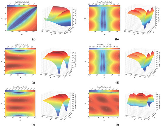
Figure 1. ${\chi }^2$ function projections over variables $A_u$, $A_d$, ${\varphi }_1$, ${\varphi }_2$. (a) Dependence of the function ${\chi }^2$ on the variables $A_u$ and $A_d$ (right graph). From the contour lines (left-hand graph), we note that the region that minimizes ${\chi }^2$ lies around a straight line at ${45}^{\circ }$. (b) Dependence of the function ${\chi }^2$ with respect to the variables $A_u$ and ${\varphi }_1$ (right-hand graph) and corresponding contour lines (left-hand graph). We note a periodicity of the maxima of the function ${\chi }^2$ with respect to the variable ${\varphi }_1$. (c) Dependence of the function ${\chi }^2$ with respect to the variables $A_u$ and ${\varphi }_2$ (right-hand graph) and corresponding contour lines (left-hand graph). We note a periodicity of the maxima and the minima of the function ${\chi }^2$ with respect to the variable ${\varphi }_2$. (d) Dependence of the function ${\chi }^2$ with respect to the variables $A_d$ and ${\varphi }_1$ (right-hand graph) and corresponding contour lines (left-hand graph). We note a periodicity of the maxima of the function ${\chi }^2$ with respect to the variable ${\varphi }_1$. (e) Dependence of the function ${\chi }^2$ with respect to the variables $A_d$ and ${\varphi }_2$ (right-hand graph) and corresponding contour lines (left-hand graph). We note a periodicity of the maxima and the minima of the function ${\chi }^2$ with respect to the variable ${\varphi }_2$. (f) Dependence of the function ${\chi }^2$ on the variables ${\varphi }_1$ and ${\varphi }_2$ (right-hand graph) and corresponding contour lines (left-hand graph).

The following color code has been established; regions towards the intense red color mean larger values of ${\chi }^2\left(X\right)$, while regions towards the intense blue color correspond to smaller values of ${\chi }^2\left(X\right)$. We point out that the function to optimize ${\chi }^2\left(X\right):R^4\to R$ is defined on (17) with variables $A_u$, $A_d$, ${\varphi }_1$, ${\varphi }_2$ bounded on the boundaries $[m_c,m_t]$, $[m_s,m_b]$, $[0,2\pi ]$, $[0,2\pi ]$, and as can be observed from the graphs (Figure 1), the topography that it is intended to optimize is rugged. With this, one sees the opportunity to explore the use of alternative optimization techniques such as bio-inspired algorithms.

3. Review of PSO, DE, and DEPSO

3.1. Particle Swarm Optimization

The particle swarm optimization (PSO) algorithm [47] is one of the most popular swarm intelligence-based algorithms. It models the behavior of groups of individuals, such as flocks, to solve complex optimization problems in D-dimensional space. The algorithm performs a search for the global optimum using a swarm of $NP$ particles. For the i-th particle of the swarm $X_{i,t}$ ($i=1,2,\dots ,NP$), its position and velocity at iteration t are represented by $X_{i,t}=\{x_{i,t}^1,x_{i,t}^2,\dots ,x_{i,t}^D\}$ and $V_{i,t}=\{v_{i,t}^1,v_{i,t}^2,\dots ,v_{i,t}^D\}$, respectively. At each iteration, the position and velocity of each particle is updated, taking into account the information of the best solution found by the swarm $X_{gbest,t}$ and the best solution found individually, $X_{pbest,t}$, by each particle. In the standard version of the PSO algorithm, the way in which the updating of the position and velocity of each particle is performed is carried out according to the following expressions [48]:

$$V_{i,t+1}=\omega ·V_{i,t}+c_1·r_1·(X_{gbest,t}-X_{i,t})+c_2·r_2·(X_{pbest,t}-X_{i,t})$$

(18)

$$X_{i,t+1}=X_{i,t}+V_{i,t+1}$$

(19)

where $c_1$ and $c_2$ are the social and cognitive coefficients, respectively, which commonly take the values $c_1=c_2=2$. $r_1$ and $r_2$ are two randomly selected values within the interval $[0,1]$. $\omega$ is known as the inertia parameter and it aims to provide a better balance between global and local search. The inertia parameter $\omega$ is updated at each iteration as follows:

$$\omega ={\omega }_{max}-{\displaystyle \frac{t·({\omega }_{max}-{\omega }_{min})}{t_{max}}}$$

(20)

where t refers to the current iteration, $t_{max}$ is the maximum number of iterations, and $t_{min}$ and $t_{max}$ are the minimum and maximum values of the inertia factor, which are generally set to values $t_{min}=0.4$ and $t_{max}=0.9$.

3.2. Differential Evolution

The DE algorithm proposed by Storn and Price [49,50] is one of the most representative evolutionary algorithms, which, due to its ease of implementation, effectiveness, and robustness, has been widely used in the solution of several complex optimization problems [51,52]. This algorithm makes use of a population P constituted from $NP$ individuals or parameter vectors:

$$P_t=\{X_{1,t},X_{2,t},\dots ,X_{i,t}\},i=1,\dots ,NP$$

(21)

where t refers to the current iteration and each individual $X_{i,t}=\{x_{i,t}^1,x_{2,t}^2,\dots ,x_{i,t}^D\}$ has D dimensions. At the beginning of the execution of this algorithm, the population is initialized randomly within the search space of the problem.

The DE algorithm consists mainly of three operators: mutation, crossover, and selection. These operators allow the algorithm to perform the search for the global optimum. Mutation, crossover, and selection are applied consecutively to each individual $X_{i,t}$ of the population $P_t$ in each of the t iterations until a certain stopping criterion is satisfied. Within the mutation, in each iteration and for each individual, a mutated vector $V_{i,t}$ is generated by means of the information of the current population $P_t$ and the application of a mutation scheme. In the standard version of the DE algorithm, the mutated vector is generated following the DE/rand/1 mutation scheme, described as follows:

$$V_{i,t}=X_{r1,t}+F·(X_{r2,t}-X_{r3,t})$$

(22)

where the indices $r_1,r_2$, and $r_3$ are randomly selected within the range $[1,NP]$ such that they are different from each other and different from the index i. $F>0$ is the scaling factor and is one of the parameters of the algorithm. The value of parameter F is typically within the interval $[0,1]$.

The next stage within the DE algorithm consists of the crossover, in which a test vector $U_{i,t}$ is generated; that is, once the mutated vector $V_{i,t}$ is generated for the individual $X_{i,t}$, the information crossover between the vector $X_{i,t}$ and the vector $V_{i,t}$ is performed. This crossover operation is performed consistently following the binomial crossover:

$$U_{i,t}^j=\left\{\begin{array}{cc}{V}_{i,t}^j\hfill & \mathrm{if}rand[0,1]<Cr\mathrm{or}j=j_{\mathrm{rand}}\hfill \\ X_{i,t}^j\hfill & \mathrm{otherwise}\hfill \end{array}\right.$$

(23)

where $rand[0,1]$ is a number uniformly selected within the interval $[0,1]$ and $j_{\mathrm{rand}}$ is an index corresponding to a variable that is uniformly selected in the interval $[1,D]$. Here, $Cr\in [0,1]$ is known as the crossover probability, and like F, it is another parameter of the algorithm.

Once the corresponding test vector $U_{i,t}$ is generated for the individual $X_{i,t}$, a selection procedure is carried out from which the population for iteration $t+1$ is constructed. The standard way to perform this selection procedure consists of comparing the fit value of the test vector $U_{i,t}$ against the fit value of the individual $X_{i,t}$, always keeping the individual with the best fit value. This procedure is performed as follows:

$$X_{i,t+1}=\left\{\begin{array}{cc}{U}_{i,t}\hfill & \mathrm{if}f\left(U_{i,t}\right)<f\left(X_{i,t}\right)\hfill \\ X_{i,t}\hfill & \mathrm{otherwise}\hfill \end{array}\right.$$

(24)

3.2.1. Improvements on DE Parameters Control

One of the components that influence the performance of the DE algorithm is the control of the F and $Cr$ parameters [32,53]. The standard version of the DE algorithm uses fixed values for these two parameters; however, the selection of these parameters can be done deterministically (following a certain rule that modifies these values after a certain number of iterations), adaptively (according to the feedback of the search process), and in a self-adaptive way (by means of the evolution information provided by the individuals of the population) [37]. One of the most representative variants concerning the improvement of the control of the parameters F and $Cr$ of the DE algorithm is proposed in the SHADE algorithm [32].

Precisely, in each iteration of the SHADE algorithm, the parameters F and $Cr$, which are associated with test vectors with a better fit than their parent vector, are stored in two sets: $S_F$ and $S_{Cr}$, respectively. Two archives or memories, $M_F$ and $M_{Cr}$ with a defined time H, and whose contents $M_{Cr,k}$ and $M_{F,k}$$(k=1,\dots ,H)$ are initialized with a value of $0.5$, serve to generate the parameters $F_i$ and $C{r}_i$ of the i-th individual $X_{i,t}$ at each iteration t. The way to generate the values of these parameters requires the uniform selection of an index, $r_i\in [1,H]$, and is carried out according to the following expressions:

$$C{r}_i={\mathrm{randn}}_i(M_{Cr,r_i},0.1)$$

(25)

$$F_i={\mathrm{randc}}_i(M_{F,r_i},0.1)$$

(26)

where $M_{CR,r_i}$ is the element selected from $M_{Cr}$ to generate the value of $C{r}_i$, while $M_{F,r_i}$ is the element selected from $M_F$ to generate the value of $F_i$; ${\mathrm{randn}}_i(M_{Cr,r_i},0.1)$ represents a normal distribution with mean $M_{CR,r_i}$ and standard deviation $0.1$, while ${\mathrm{randc}}_i(M_{F,r_i},0.1)$ represents a Cauchy distribution with parameter position $M_{F,r_i}$ and scale factor $0.1$. When generating the value of the parameter $C{r}_i$, it must be verified that it is within the range $[0,1]$; otherwise, if $C{r}_i<0$ then $C{r}_i$ is truncated to 0 and if $C{r}_i>1$ then $C{r}_i$ is truncated to 1. For the parameter $F_i$, if $F_i>1$ then $F_i$ is truncated to 1, otherwise, if $F_i<0$ then $F_i$ is regenerated until $F_i>0$.

At the end of each iteration, the contents of the $M_{Cr}$ and $M_F$ memories are updated as follows:

$$M_{Cr,k,t+1}=\left\{\begin{array}{cc}mea{n}_{WL}\left(S_{Cr}\right),\hfill & \mathrm{si}{S}_{Cr}\ne \varnothing \hfill \\ M_{Cr,k,t},\hfill & \mathrm{otherwise}\hfill \end{array}\right.$$

(27)

$$M_{F,k,t+1}=\left\{\begin{array}{cc}mea{n}_{WL}\left(S_F\right),\hfill & \mathrm{si}{S}_F\ne \varnothing \hfill \\ M_{F,k,t},\hfill & \mathrm{otherwise}\hfill \end{array}\right.$$

(28)

where $mea{n}_{WL}\left(S\right)$ is the Lehmer weighted mean defined by the means of Equation (29), and S refers to $S_{Cr}$ or $S_F$.

$$mea{n}_{WL}={\displaystyle \frac{{\displaystyle \sum _{k=1}^{\left|S\right|}}{w}_k·S_k^2}{{\displaystyle \sum _{k=1}^{\left|S\right|}}{w}_k·S_k}}$$

(29)

$$w_k={\displaystyle \frac{\Delta f_k}{{\displaystyle \sum _{l=1}^{\left|S\right|}}\Delta f_l}}$$

(30)

$$\Delta f_k=|f\left(X_{p,k,t}\right)-f\left(X_{k,t}\right)|$$

(31)

In Equations (27) and (28), $k\in [1,H]$ determines the position in memory to be updated. At iteration t, the k-th element in memory is updated. At the beginning of the optimization process, $k=1$ and is incremented each time a new element is added to memory. If $k>H$, k is assigned equal to 1.

Due to the good performance obtained by the SHADE algorithm when solving optimization problems using this strategy, this paper takes advantage of the adaptive control of the parameters provided by the SHADE algorithm.

3.2.2. DEPSO Algorithm

The self-adaptive differential evolution algorithm based on particle swarm optimization (DEPSO) [39] is a recent method, which incorporates characteristics of the PSO algorithm within the structure of the DE algorithm for solving numerical optimization problems. In this algorithm, the top $\alpha ·NP$$(\alpha \in [0.1,0.9\left]\right)$ of the best particles in the current iteration is used to form an elite sub-swarm $\left(P\right)$, while the rest are used to form a non-elite sub-swarm $\left(Q\right)$.

The DEPSO algorithm follows a scheme similar to the standard version of the DE algorithm, i.e., it uses mutation, crossover, and selection operators within the evolutionary process of the algorithm. Within the mutation, a mutation strategy is implemented that, in a self-adaptive way, selects between two mutation schemes to generate in each iteration a mutated vector $V_{i,t+1}$ for the i-th particle $X_{i,t}$, as follows:

$$V_{i,t+1}=\left\{\begin{array}{cc}{X}_{r1,t}^P+F_i·(X_{r2,t}^p-X_{r3,t}^Q)\hfill & \mathrm{if}rand[0,1]<S{P}_t\hfill \\ \omega ·X_{i,t}+c_1·r_1·(X_{gbest,t}-X_{i,t})\hfill \\ +c_2·r_2·(X_{pbest,t}-X_{i,t})\hfill & \mathrm{otherwise}\hfill \end{array}\right.$$

(32)

where $rand[0,1]$ is a random number selected uniformly within the interval $[0,1]$ and $S{P}_t$ represents the probability of selecting between one of the two mutation schemes. In Equation (32), the case in which $rand[0,1]<S{P}_t$ represents the form in which a novel mutation scheme denoted DE/e-rand/1 generates a mutated vector $V_{i,t+1}$. In this scheme, two optimal solutions of the elite sub-swarm $(X_{r1,t}^P$ and $X_{r2,t}^p)$ and one solution of the non-elite sub-swarm $\left(X_{r3,G}^Q\right)$ are required, and a scaling factor $F_i$ is used, which acts at the level of each particle. The remaining case represents the way in which the mutation scheme of the standard PSO algorithm is used to generate a mutated vector $V_{i,t+1}$.

The selection probability $S{P}_t$ of Equation (32) changes adaptively within the evolution of the algorithm, as follows:

$$S{P}_t={\displaystyle \frac{1}{1+e^{(1-{(t_{max}/(t+1))}^{\tau })}}}$$

(33)

where $t_{max}$ is the maximum number of iterations and t is the current iteration. $\tau$ is a positive constant.

Within the crossover operator, a test vector $U_{i,t}$ is generated by combining the information of the current particle $X_{i,t}$ and the mutated vector $V_{i,t+1}$, following the binomial crossover (see Equation (23)). The selection of the surviving particle to the next iteration is carried out by the competition between the current particle $X_{i,t}$ and the test vector $U_{i,t}$; the one with the best fit value according to the objective function is selected to remain within the next iteration.

When a particle remains stagnant over a maximum number of iterations (e.g., 5), the values of its corresponding scale factor $F_i$ and crossover probability $C{r}_i$ are reset in order to increase diversity. The way in which the values of these parameters are reset is as follows:

$$F_{i,t+1}=\left\{\begin{array}{cc}{F}_{i,t}\hfill & \mathrm{if}N{S}_i<N{S}_{max}\hfill \\ F_l+rand[0,1]·(F_u-F_l)\hfill & \mathrm{otherwise}\hfill \end{array}\right.$$

(34)

$$C{r}_{i,t+1}=\left\{\begin{array}{cc}C{r}_{i,t}\hfill & \mathrm{if}N{S}_i<N{S}_{max}\hfill \\ C{r}_l+rand[0,1]·(C{r}_u-C{r}_l)\hfill & \mathrm{otherwise}\hfill \end{array}\right.$$

(35)

where $F_i$ and $C{r}_i$ are the scaling factor and the crossover probability, respectively, of the particle $X_{i,t}$ at iteration t. $F_l=0.1$ and $F_u=0.8$ are the lower and upper bounds respectively of the scaling factor. $C{r}_l=0.3$ and $C{r}_u=1.0$ are the lower and upper bounds, respectively, of the crossover probability and $rand[0,1]$ is a random number selected within the interval $[0,1]$. $N{S}_i$ is a stagnation counter for each particle and $N{S}_{max}$ is the maximum number of iterations with stagnation.

To avoid stagnation, the DEPSO algorithm randomly updates a sub-dimension of individuals within the non-elite population $\left(Q\right)$, in which $N{S}_i>N{S}_{max}$, to reset them as follows:

$$X_{i,t}^j=\left\{\begin{array}{cc}{X}_{min}^j+rand[0,1]·(X_{max}^j-X_{min}^j)\hfill & \mathrm{if}rand{[0,1]}_j\le \gamma ,j=1,2,\dots D\hfill \\ X_{i,t}^j\hfill & \mathrm{otherwise}\hfill \end{array}\right.$$

(36)

where $rand{[0,1]}_j$ is a random number selected within the interval $[0,1]$, $\gamma$ is a probability fixed value, and $X_{min}^j$ and $X_{max}^j$ are the lower and upper limits, respectively, of the variable j.

In general, the DEPSO algorithm manages to be superior to other variants of the DE algorithm in different optimization problems. The performance of this algorithm is due to the fact that it maintains a good balance between exploration and exploitation, thanks to the use of the self-adaptive mutation strategy, in which the “DE/e-rand/1” scheme has better exploration abilities, while the mutation scheme of the PSO algorithm achieves better convergence abilities. With this strategy, the population manages to maintain a good diversity in the first stages of the evolutionary process and a faster convergence towards the last stages of the process.

4. Proposed HE-DEPSO Algorithm

Despite the development of several advanced versions of the DE algorithm in recent years, its performance still needs to improve in optimization problems with multiple local minima. To address these issues, the design of effective mutation operators and parameter control are two key aspects to improve the performance of the DE algorithm. In the proposed HE-DEPSO algorithm, an adaptive hybrid mutation operator is developed, which takes the self-adaptive mutation strategy from the DEPSO algorithm [39] as a basis and incorporates the parameter control mechanism from the SHADE algorithm [32]. This adaptive hybrid mutation operator introduces a new mutation strategy called “DE/current-to-EHE/1”, which utilizes the historical information of the elite individuals in the population to enhance the optimization of the ${\chi }^2$ function.

4.1. Adaptive Hybrid Mutation Operator

In order to achieve a better balance between exploration and exploitation, the mutation operator of the HE-DEPSO algorithm adopts a dual mechanism in which it adaptively selects between two mutation strategies. First, a new mutation strategy called “DE/current-to-EHE/1” is presented, which is oriented to improve the balance between exploration and exploitation abilities within the early stages of the evolutionary process. On the other hand, to improve the exploitation capacity within the more advanced stages of the evolutionary process, the mutation scheme of the PSO algorithm (Equation (32)) is incorporated in a similar way to the self-adaptive mutation strategy of the DEPSO algorithm (Equation (18)).

Unlike the “DE/e-rand/1” scheme used within the self-adaptive mutation strategy of the DEPSO algorithm, in which only the information of the individuals of the current iteration is used, the “DE/current-to-EHE/1” strategy uses the historical information of the elite and obsolete individuals of the evolutionary process to improve the exploration capability of the algorithm. This strategy is described below.

4.1.1. DE/Current-to-EHE/1 Mutation Strategy

Within evolutionary algorithms, the best individuals in the population, also known as elite individuals, retain valuable evolutionary information to guide the population to promising regions [39,54,55,56]. However, many of the proposals made use of the information from the elite individuals of the current iteration, completely forgetting the information from the previous elite individuals. This absence of information within subsequent iterations may limit the ability of new individuals to explore the search space. Because of this, historical evolution information is used to improve the ability to explore new individuals.

Before applying the mutation operator, all individuals in the current population $P_t$ are sorted in ascending order based on their fitness values. After reordering the population, two partitions of individuals are created. The first partition, denoted by ${\mathrm{E}}_{\mathrm{t}}$, consists of the top $pb\%\in [0.1,1]$ best individuals or elite individuals. The second partition, denoted by NE_t, groups all non-elite individuals, i.e., $NP-NP·pb\%$. It is important to note that E_t∪ NE_t = $P_t$.

Unlike other mutation strategies [36,39,57], in which only elite individuals corresponding to the current iteration are used, this strategy makes use of the evolution history by incorporating two external archives of size $NP$. The first archive, denoted by HE, stores at each iteration the elite individuals belonging to the E_t partition. If the size of the archive HE is greater than $NP$ then its size is readjusted. The second archive used, denoted by HL, stores the obsolete individuals (individuals discarded within the selection process) and is updated at each iteration. Similar to the HE archive, if the size of the HL file is larger than $NP$ then its size is reset. With the information of the individuals belonging to E_t and HE, a group of candidates can be formed using E_t∪ HE to mutate individuals in the population. On the other hand, the individuals of NE_t and HL make up a group of individuals NE_t∪ HL, whose information contributes to the exploration of the search space. The way in which a mutated vector is generated by the “DE/current-to-EHE/1” strategy is as follows:

$$V_{i,t}=X_{i,t}+F_i·(X_{E_r,t}-X_{i,t})+F_i·(X_{P_r,t}-X_{H{L}_r,t})$$

(37)

where $X_{i,t}$ is the i-th individual at iteration t, $X_{E_r,t}$ is a randomly selected individual from among the individuals in the group E_t∪ HE, $X_{P_r,t}$ is an individual randomly selected from within the current population $P_t$, $X_{H{L}_r,t}$ is an individual randomly selected from the individuals comprising the group NE_t∪ HL, and $F_i$ is the scaling factor corresponding to the i-th individual.

Following Equation (37), it is possible to observe that the “DE/current-to-EHE/1” strategy can help the HE-DEPSO algorithm to maintain a good exploration capability and direct the mutated individuals to promising regions without leading to stagnation in local minima. This can be explained as follows:

• The use of a randomly selected individual within the group E_t ∪ HE, i.e., $X_{E_r,t}$, helps to guide mutated individuals to more promising regions. However, due to the presence of the historical information of the elite individuals (HE), the mutated individuals are prevented from being directed towards the best regions found, thus allowing the maintenance of good diversity in the population and increasing the chances of targeting optimal regions.
• The participation of two individuals, $X_{P_r,t}$ and $X_{L_r,t}$, randomly selected from $P_t$ and HL, respectively, promotes the diversity of mutated individuals. Consequently, the search diversity of the HE-DEPSO algorithm is considerably improved, which is beneficial for escaping from possible local minima.

At the beginning of the execution of the HE-DEPSO algorithm, the archives HE and HL are defined as empty. Through the evolutionary process, they store the elite and obsolete individuals, respectively. When analyzing the effect of the parameter $pb\%$, which determines the percentage of individuals within the participation of E_t, it was found that values close to $0.9$ promote the participation of a more significant number of elite individuals, causing a greater diversity in the population. However, this diversity increase may affect the HE-DEPSO algorithm’s convergence capability. On the other hand, values close to $0.1$ may restrict the number of elite individuals to be considered, which improves the convergence of the algorithm but may cause stagnation at local minima. Due to the above, within the HE-DEPSO algorithm we choose to update in each iteration the value of $pb\%$ following a linear decrement, given as follows:

$$pb\%=p_{max}-{\displaystyle \frac{t·(p_{max}-p_{min})}{t_{max}}}$$

(38)

where t refers to the current iteration, $t_{max}$ is the maximum number of iterations, and $p_{min}$ and $p_{max}$ are the minimum and maximum values of the interval assigned for the percentage of individuals within the partition E_t. In this work, we have chosen to use the values $p_{max}=0.4$ and $p_{min}=0.1$. In this way, the sensitivity of the $pb\%$ parameter is reduced and, at the same time, a good balance between exploitation and exploration is maintained.

4.1.2. Selection of Mutation Strategy for Adaptive Hybrid Mutation Operator

The adaptive hybrid mutation operator implemented in the HE-DEPSO algorithm uses two mutation strategies that aim to improve the exploration and exploitation abilities of the HE-DEPSO algorithm at different stages of the evolutionary process. Concretely, for each individual $X_{i,t}$ in the population, this operator generates a mutated vector $V_{i,t}$ as follows:    

$$V_{i,t}=\left\{\begin{array}{cc}{X}_{i,t}+F_i·(X_{E_r,t}-X_{i,t})+F_i·(X_{P_r,t}-X_{H{L}_r,t})\hfill & \mathrm{if}rand[0,1]<{\alpha }_t\hfill \\ \omega ·X_{i,t}+c_1·r_1·(X_{gbest,t}-X_{i,t})\hfill \\ +c_2·r_2·(X_{pbest,t}-X_{i,t})\hfill & \mathrm{otherwise}\hfill \end{array}\right.$$

(39)

where $rand[0,1]$ is a random number selected uniformly within the interval $[0,1]$ and ${\alpha }_t$ represents the probability of selecting between the “DE/current-to-EHE/1” mutation strategy and the adopted mutation strategy of the PSO algorithm (Equation (18)).

The probability of selection ${\alpha }_t$ is updated at each iteration according to Equation (33), taking a value of $\tau =1.8$. Figure 2 shows the mutation strategy selection curve followed by the adaptive hybrid mutation operator of the HE-DEPSO algorithm. The probability selection curve described by Equation (33) with a value of $\tau =1.8$, for a maximum number of iterations $t_{max}$, is illustrated in red in Figure 2a. On the other hand, Figure 2b shows, as an example, a possible distribution of occurrences among which is selected the mutation strategy “DE/current-to-EHE/1” (squares in blue color) or the adopted strategy of the PSO algorithm (circles in magenta color). According to these graphs, it can be observed that, within the first stages of evolution of the HE-DEPSO algorithm, the probability of selection ${\alpha }_t$ tends towards values close to 1, which increases the probability that the mutation strategy “DE/current-to-EHE/1” is selected, and the balance between exploration and exploitation provided by this strategy is taken advantage of. On the other hand, towards the advanced stages of the algorithm evolution, the mutation strategy adopted from the PSO algorithm is selected more frequently; this implies that, during the advanced stages, there is a higher probability that the HE-DEPSO algorithm increases its exploitation ability due to more frequent use of the information of the best positions of each individual, as well as the information of the position of the best individual in the population.

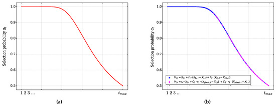
Figure 2. Strategy selection curve; (a) Selection probability ${\alpha }_t$, (b) Distribution of strategy selection.

4.2. The Complete HE-DEPSO Algorithm

The HE-DEPSO algorithm follows the usual structure of the DE algorithm in general, in which we have the stages of mutation, crossover, and selection. After generating a mutated vector $V_{i,t}$ for the i-th individual of the population, as described in the previous section, we proceed to generate a test vector $U_{i,t}$ for the individual $X_{i,t}$ using the binomial crossover (Equation (23)). In order to reduce the sensitivity of the F and $C_r$ parameter controls, the HE-DEPSO algorithm takes advantage of the individual-level adaptive parameter control of the SHADE algorithm to generate the parameter configuration of F and $C_r$ for each individual. Finally, in the selection stage, the individuals that would make up the population for the next iteration are identified; this is done according to Equation (24). Based on the above description, the pseudocode of the complete HE-DEPSO is reported in Algorithm 1.

Algorithm 1: The pseudocode of HE-DEPSO

4.3. Complexity Analysis of the HE-DEPSO Algorithm

The logical operations of HE-DEPSO are simple, so its computational complexity is low. The analysis uses the big-$\mathcal{O}$ notation. The initialization of the NP individuals has a complexity of $\mathcal{O}(NP·D)$. The evaluation of the cost function is $\mathcal{O}\left(NP\right)$, and the sorting of $NP$ individuals has a complexity of $\mathcal{O}(NP·logNP)$. Updating the values of each individual depends on mutation and crossover operations, each with a complexity of $\mathcal{O}\left(D\right)$, so the update of the individuals is given by $\mathcal{O}\left(NP\right(1+logNP+2D\left)\right)$. Thus, the total complexity of HE-DEPSO is $\mathcal{O}(t_{max}·NP(1+logNP+2D))$. This complexity is similar to the computational cost of recent DE variants (CoDE, SHADE, and DEPSO) proposed for global optimization; therefore, HE-DEPSO has similar execution times to these variations [30,32,39].

5. Experimental Results and Analysis

This section verifies the performance of the proposed HE-DEPSO algorithm in solving different optimization problems. First, the set of test problems used is presented, then the algorithms selected to carry out comparisons are presented, as well as the configuration of their parameters. Then, the performance of the HE-DEPSO algorithm is compared against the selected algorithms within the test problem set. Finally, a discussion of the results obtained is presented.

5.1. Benchmark Functions

In order to validate the performance of the HE-DEPSO algorithm in solving different optimization problems, the set of single-objective test functions with boundary constraints CEC 2017 [58] was used. This set consists of 29 test functions whose global optimum is known. We have two unimodal functions $(F_1$ and $F_3)$, seven simple multimodal functions $(F_4-F_{10})$, ten hybrid functions $(F_{11}-F_{20})$, and ten composite functions $(F_{21}-F_{30})$. In all these optimization problems, we seek to find the global minimum ($F_{min}$) within the search space bounded in each dimension $\left(D\right)$ by the interval $[-100,100]$. Information about this set of test functions is briefly presented in Table 2.

Table 2. Details of benchmark functions used in the experiments.

Function Type	Index	Function Name	Optimum $\mathbf{\left(}{\mathit{F}}_{\mathit{min}}\mathbf{\right)}$
Unimodal	1	Shifted and Rotated Bent Cigar	100
Functions	3	Shifted and Rotated Zakharov	300
	4	Shifted and Rotated Rosenbrock	400
	5	Shifted and Rotated Rastrigin	500
Simple	6	Shifted and Rotated Expanded Schaffer F6	600
Multimodal	7	Shifted and Rotated Lunacek Bi-Rastrigin	700
Functions	8	Shifted and Rotated Non-Continuous Rastrigin	800
	9	Shifted and Rotated Levy	900
	10	Shifted and Rotated Schwefel	1000
	11	Hybrid Problem 1 (N = 3)	1100
	12	Hybrid Problem 2 (N = 3)	1200
	13	Hybrid Problem 3 (N = 3)	1300
Hybrid	14	Hybrid Problem 4 (N = 4)	1400
Functions	15	Hybrid Problem 5 (N = 4)	1500
	16	Hybrid Problem 6 (N = 4)	1600
	17	Hybrid Problem 7 (N = 5)	1700
	18	Hybrid Problem 8 (N = 5)	1800
	19	Hybrid Problem 9 (N = 5)	1900
	20	Hybrid Problem 10 (N = 6)	2000
	21	Composition Problem 1 (N = 3)	2100
	22	Composition Problem 2 (N = 3)	2200
	23	Composition Problem 3 (N = 4)	2300
Composition	24	Composition Problem 4 (N = 4)	2400
Functions	25	Composition Problem 5 (N = 5)	2500
	26	Composition Problem 6 (N = 5)	2600
	27	Composition Problem 7 (N = 6)	2700
	28	Composition Problem 8 (N = 6)	2800
	29	Composition Problem 9 (N = 9)	2900
	30	Composition Problem 10 (N = 3)	3000

5.2. Algorithms and Parameter Settings

In this subsection, HE-DEPSO is compared with five algorithms, including the PSO and DE algorithms, as well as three representative and advanced variants of the DE algorithm, named CoDE [30], SHADE [32], and DEPSO [39]. Among these algorithms, CoDE and DEPSO incorporate modifications mainly within the mutation operator of the DE algorithm, while SHADE modifies the control of the F and $Cr$ parameters. The performance comparison of the HE-DEPSO algorithm with the previously mentioned algorithms was performed in two dimensions, $D=10$ and $D=30$, on the CEC 2017 test function set.

In order to ensure a fair comparison, the parameter settings in common to all algorithms were assigned identically: the maximum number of iterations, $t_{max}$, was set to 1000, the population size, $NP$, to 100, and 31 independent runs were performed. The configuration of each algorithm’s parameters followed the values suggested by their respective authors, as presented in Table 3. The proposed HE-DEPSO algorithm was implemented in Python version 3.11, and all algorithms were executed on the same computer with 8 GB of RAM and a six-core 3.6 GHz processor.

Table 3. Parameter settings of all algorithms.

Algorithm	Parameters
HE-DEPSO	$p_{min}=0.1$, $p_{max}=0.4$, $\tau =1.8$, $c1=c2=2$, $\omega \in [0.4,0.9]$,
	$H=NP$, $M_F(1:H)=0.5$, $M_{Cr}(1:H)=0.8$
DEPSO	$c1=c2=2$, $\omega \in [0.4,0.9]$, $Cr[0.3,1.0]$, $F[0.1,0.8]$,
	$N{S}_{max}=5$, $\gamma =0.001$, $\tau =1.8$, $SEP=0.3·NP$
SHADE	$H=NP$, $M_F(1:H)=M_{Cr}(1:H)=0.5$
CoDE	(1) $[F=1.0,Cr=0.1]$, (2) $[F=1.0,Cr=0.9]$, (3) $[F=0.8,Cr=0.2]$
DE	$Cr=0.9$, $F=0.5$
PSO	$\omega \in [0.4,0.9]$, $c1=c2=2$

5.3. Comparison with DE, PSO, and Three State-of-the-Art DE Variants

In order to evaluate the performance of the HE-DEPSO algorithm, its optimization results and convergence properties are compared and analyzed with respect to those obtained by the algorithms DE, PSO, CoDE, SHADE, and DEPSO, on the set of CEC 2017 test functions.

Table 4 and Table 5 report the statistical results for each algorithm at $D=10$ and $D=30$, respectively. The error measure of the solution $|F_{min}-F\left(X^{*}\right)|$, where $F_{min}$ is the known solution of the problem and $X^{*}$ is the best solution found in each iteration of each algorithm, was used to obtain these results. These tables show the mean and standard deviation (Std) of the solution error measure for each function and algorithm over the 31 independent runs and the ranking achieved based on the mean value obtained. The best results are highlighted in bold.

Table 4. Comparison of results between HE-DEPSO, DE, PSO, and three advanced variants of the DE algorithm on the set of CEC 2017 test functions with $D=10$.

Function	Metrics	HE-DEPSO	DEPSO	SHADE	CoDE	DE	PSO
$F_1$	Mean	0.0000	1.8337 $\times {10}^{-15}$	0.0000	1.1580 $\times {10}^{-10}$	3.5103 $\times {10}^{-5}$	1.1366 $\times {10}^{10}$
	Std	0.0000	4.8427 $\times {10}^{-15}$	0.0000	6.0507 $\times {10}^{-11}$	2.0793 $\times {10}^{-5}$	9.7631 $\times {10}^9$
	Rank	1	4	1	3	2	5
	Significance		≈	≈	+	+	+
$F_3$	Mean	9.1683 $\mathbf{\times } {\mathbf{10}}^{\mathbf{-}\mathbf{16}}$	1.3752 $\times {10}^{-14}$	1.6503 $\times {10}^{-14}$	2.0001 $\times {10}^{-9}$	1.7359 $\times {10}^{-4}$	1.5886 $\times {10}^{10}$
	Std	0.0000	0.0000	0.0000	2.7390 $\times {10}^{-11}$	4.8441 $\times {10}^{-4}$	6.2297 $\times {10}^2$
	Rank	1	1	1	2	3	4
	Significance		≈	≈	+	+	+
$F_4$	Mean	0.0000	2.3838 $\times {10}^{-14}$	2.0805 $\times {10}^0$	2.3103 $\times {10}^{-9}$	1.0409 $\times {10}^{-3}$	5.8071 $\times {10}^1$
	Std	0.0000	2.8513 $\times {10}^{-14}$	6.7544 $\times {10}^{-1}$	1.2601 $\times {10}^{-9}$	6.4578 $\times {10}^{-4}$	6.9704 $\times {10}^1$
	Rank	1	2	5	3	4	6
	Significance		+	+	+	+	+
$F_5$	Mean	2.8439 $\mathbf{\times } {\mathbf{10}}^{\mathbf{0}}$	4.0119 $\times {10}^0$	3.8489 $\times {10}^0$	8.5594 $\times {10}^0$	2.9710 $\times {10}^1$	3.0728 $\times {10}^1$
	Std	7.2094 $\mathbf{\times } {\mathbf{10}}^{\mathbf{-}\mathbf{1}}$	1.6940 $\times {10}^0$	1.0401 $\times {10}^0$	1.4246 $\times {10}^0$	3.9355 $\times {10}^0$	1.2073 $\times {10}^1$
	Rank	1	3	2	4	5	6
	Significance		+	+	+	+	+
$F_6$	Mean	0.0000	4.6321 $\times {10}^{-3}$	2.7530 $\times {10}^{-4}$	4.6895 $\times {10}^{-3}$	4.5748 $\times {10}^{-5}$	1.1970 $\times {10}^1$
	Std	0.0000	2.5790 $\times {10}^{-2}$	5.5026 $\times {10}^{-4}$	2.4954 $\times {10}^{-3}$	2.2095 $\times {10}^{-5}$	9.6167 $\times {10}^0$
	Rank	1	4	3	5	2	6
	Significance		+	+	+	+	+
$F_7$	Mean	1.2678 $\mathbf{\times } {\mathbf{10}}^{\mathbf{1}}$	2.1067 $\times {10}^1$	1.3953 $\times {10}^1$	2.0678 $\times {10}^1$	3.9143 $\times {10}^1$	3.0657 $\times {10}^1$
	Std	7.0313 $\times {\mathbf{10}}^{\mathbf{-}\mathbf{1}}$	6.7134 $\times {10}^0$	7.6551 $\times {10}^{-1}$	2.2560 $\times {10}^0$	3.7389 $\times {10}^0$	8.6791 $\times {10}^0$
	Rank	1	4	2	3	6	5
	Significance		+	+	+	+	+
$F_8$	Mean	2.2853 $\mathbf{\times } {\mathbf{10}}^{\mathbf{0}}$	4.2045 $\times {10}^0$	3.8070 $\times {10}^0$	8.6884 $\times {10}^0$	2.6037 $\times {10}^1$	2.4833 $\times {10}^1$
	Std	8.1114 $\times {10}^{-1}$	1.9346 $\times {10}^0$	7.3957 $\mathbf{\times } {\mathbf{10}}^{\mathbf{-}\mathbf{1}}$	1.8765 $\times {10}^0$	5.5290 $\times {10}^0$	1.1493 $\times {10}^1$
	Rank	1	3	2	4	6	5
	Significance		+	+	+	+	+
$F_9$	Mean	0.0000	7.3346 $\times {10}^{-15}$	0.0000	0.0000	0.0000	6.8233 $\times {10}^1$
	Std	0.0000	2.8391 $\times {10}^{-14}$	0.0000	0.0000	0.0000	1.9812 $\times {10}^2$
	Rank	1	2	1	1	1	3
	Significance		≈	≈	≈	+	+
$F_{10}$	Mean	2.4499 $\times {10}^2$	8.9742 $\times {10}^2$	1.5812 $\mathbf{\times } {\mathbf{10}}^{\mathbf{2}}$	7.4438 $\times {10}^2$	1.4730 $\times {10}^3$	9.1356 $\times {10}^2$
	Std	1.1864 $\times {10}^2$	1.6890 $\times {10}^2$	7.6565 $\mathbf{\times } {\mathbf{10}}^{\mathbf{1}}$	1.1745 $\times {10}^2$	1.7509 $\times {10}^2$	3.3829 $\times {10}^2$
	Rank	2	4	1	3	6	5
	Significance		+	−	+	≈	+
$F_{11}$	Mean	2.5687 $\mathbf{\times } {\mathbf{10}}^{\mathbf{-}\mathbf{7}}$	8.6658 $\times {10}^{-1}$	2.3208 $\times {10}^0$	1.2502 $\times {10}^0$	6.7909 $\times {10}^0$	8.1368 $\times {10}^1$
	Std	1.4103 $\mathbf{\times } {\mathbf{10}}^{\mathbf{-}\mathbf{6}}$	6.1559 $\times {10}^{-1}$	4.7869 $\times {10}^{-1}$	4.6467 $\times {10}^{-1}$	9.9142 $\times {10}^{-1}$	8.3317 $\times {10}^1$
	Rank	1	2	4	3	5	6
	Significance		+	+	+	+	+
$F_{12}$	Mean	8.1966 $\times {10}^1$	1.1535 $\mathbf{\times } {\mathbf{10}}^{\mathbf{1}}$	3.5298 $\times {10}^1$	2.7652 $\times {10}^2$	5.3458 $\times {10}^2$	8.7444 $\times {10}^7$
	Std	7.0615 $\times {10}^1$	2.8045 $\times {10}^1$	1.4666 $\mathbf{\times } {\mathbf{10}}^{\mathbf{1}}$	6.4786 $\times {10}^1$	1.2345 $\times {10}^2$	3.8318 $\times {10}^8$
	Rank	3	1	2	4	5	6
	Significance		−	−	+	+	+
$F_{13}$	Mean	3.8882 $\mathbf{\times } {\mathbf{10}}^{\mathbf{0}}$	4.6716 $\times {10}^0$	5.9948 $\times {10}^0$	1.1231 $\times {10}^1$	1.2796 $\times {10}^1$	6.3448 $\times {10}^3$
	Std	2.4042 $\times {10}^0$	9.7586 $\times {10}^{-1}$	6.0682 $\mathbf{\times } {\mathbf{10}}^{\mathbf{-}\mathbf{1}}$	2.0901 $\times {10}^0$	1.7030 $\times {10}^0$	1.2009 $\times {10}^4$
	Rank	1	2	3	4	5	6
	Significance		≈	+	+	+	+
$F_{14}$	Mean	2.4091 $\mathbf{\times } {\mathbf{10}}^{\mathbf{0}}$	6.8868 $\times {10}^0$	1.9065 $\times {10}^1$	2.0295 $\times {10}^1$	2.6185 $\times {10}^1$	1.7551 $\times {10}^2$
	Std	5.1573 $\times {10}^0$	8.0249 $\times {10}^0$	3.0340 $\times {10}^0$	1.2717 $\mathbf{\times } {\mathbf{10}}^{\mathbf{-}\mathbf{1}}$	1.2365 $\times {10}^0$	9.5615 $\times {10}^1$
	Rank	1	2	3	4	5	6
	Significance		+	+	+	+	+
$F_{15}$	Mean	3.6646 $\mathbf{\times } {\mathbf{10}}^{\mathbf{-}\mathbf{1}}$	5.7132 $\times {10}^{-1}$	1.0838 $\times {10}^0$	1.3990 $\times {10}^0$	2.1239 $\times {10}^0$	4.6041 $\times {10}^2$
	Std	2.3145 $\mathbf{\times } {\mathbf{10}}^{\mathbf{-}\mathbf{1}}$	4.9456 $\times {10}^{-1}$	3.3723 $\times {10}^{-1}$	5.4455 $\times {10}^{-1}$	1.2934 $\times {10}^0$	1.0508 $\times {10}^3$
	Rank	1	2	3	4	5	6
	Significance		+	+	+	+	+
$F_{16}$	Mean	1.4450 $\mathbf{\times } {\mathbf{10}}^{\mathbf{0}}$	1.6357 $\times {10}^0$	4.5365 $\times {10}^0$	4.3009 $\times {10}^0$	1.9028 $\times {10}^1$	1.2496 $\times {10}^2$
	Std	3.2202 $\mathbf{\times } {\mathbf{10}}^{\mathbf{-}\mathbf{1}}$	3.2942 $\times {10}^0$	2.2215 $\times {10}^0$	2.5242 $\times {10}^0$	1.6484 $\times {10}^1$	1.0780 $\times {10}^2$
	Rank	1	2	4	3	5	6
	Significance		−	+	+	+	+
$F_{17}$	Mean	7.2016 $\mathbf{\times } {\mathbf{10}}^{\mathbf{0}}$	1.2075 $\times {10}^1$	2.1001 $\times {10}^1$	2.0112 $\times {10}^1$	2.8168 $\times {10}^1$	5.7710 $\times {10}^1$
	Std	3.0221 $\times {10}^0$	8.5311 $\times {10}^0$	3.2211 $\times {10}^0$	2.8326 $\times {10}^0$	1.8397 $\mathbf{\times } {\mathbf{10}}^{\mathbf{0}}$	2.4017 $\times {10}^1$
	Rank	1	2	4	3	5	6
	Significance		+	+	+	+	+
$F_{18}$	Mean	3.8770 $\mathbf{\times } {\mathbf{10}}^{\mathbf{-}\mathbf{1}}$	8.2949 $\times {10}^0$	1.9823 $\times {10}^1$	2.0117 $\times {10}^1$	2.0542 $\times {10}^1$	2.7241 $\times {10}^4$
	Std	1.4583 $\times {10}^{-1}$	6.7399 $\times {10}^0$	1.9348 $\times {10}^0$	3.4569 $\times {10}^{-2}$	1.0532 $\mathbf{\times } {\mathbf{10}}^{\mathbf{-}\mathbf{1}}$	1.8731 $\times {10}^4$
	Rank	1	2	3	4	5	6
	Significance		+	+	+	+	+
$F_{19}$	Mean	9.7895 $\mathbf{\times } {\mathbf{10}}^{\mathbf{-}\mathbf{2}}$	5.4625 $\times {10}^{-1}$	1.0349 $\times {10}^0$	5.9210 $\times {10}^{-1}$	1.2208 $\times {10}^0$	5.0978 $\times {10}^3$
	Std	1.2871 $\mathbf{\times } {\mathbf{10}}^{\mathbf{-}\mathbf{1}}$	3.7564 $\times {10}^{-1}$	1.5715 $\times {10}^{-1}$	4.4716 $\times {10}^{-2}$	2.0310 $\times {10}^{-1}$	1.1584 $\times {10}^4$
	Rank	1	2	4	3	5	6
	Significance		+	+	+	+	+
$F_{20}$	Mean	5.2046 $\mathbf{\times } {\mathbf{10}}^{\mathbf{0}}$	6.9310 $\times {10}^0$	1.7787 $\times {10}^1$	2.0000 $\times {10}^1$	2.5137 $\times {10}^1$	5.9825 $\times {10}^1$
	Std	3.1153 $\times {10}^0$	6.8469 $\times {10}^0$	3.9314 $\times {10}^0$	1.4932 $\mathbf{\times } {\mathbf{10}}^{\mathbf{-}\mathbf{4}}$	1.9501 $\times {10}^0$	4.0129 $\times {10}^1$
	Rank	1	2	3	4	5	6
	Significance		≈	+	+	+	+
$F_{21}$	Mean	1.7676 $\times {10}^2$	1.0695 $\mathbf{\times } {\mathbf{10}}^{\mathbf{2}}$	1.5575 $\times {10}^2$	1.2554 $\times {10}^2$	1.9598 $\times {10}^2$	1.9045 $\times {10}^2$
	Std	4.6029 $\times {10}^1$	2.0972 $\mathbf{\times } {\mathbf{10}}^{\mathbf{1}}$	4.2795 $\times {10}^1$	4.8087 $\times {10}^1$	5.7606 $\times {10}^1$	6.2148 $\times {10}^1$
	Rank	4	1	3	2	6	5
	Significance		−	−	−	+	+
$F_{22}$	Mean	1.0000 $\times {10}^2$	9.7428 $\times {10}^1$	9.9647 $\times {10}^1$	7.4280 $\mathbf{\times } {\mathbf{10}}^{\mathbf{1}}$	1.0070 $\times {10}^2$	1.2711 $\times {10}^2$
	Std	0.0000	1.5939 $\times {10}^1$	2.1997 $\times {10}^0$	4.4524 $\times {10}^1$	5.7442 $\times {10}^{-1}$	5.6792 $\times {10}^1$
	Rank	4	2	3	1	5	6
	Significance		+	+	≈	≈	+
$F_{23}$	Mean	3.0613 $\mathbf{\times } {\mathbf{10}}^{\mathbf{2}}$	3.0845 $\times {10}^2$	3.0859 $\times {10}^2$	3.2072 $\times {10}^2$	3.3600 $\times {10}^2$	3.4479 $\times {10}^2$
	Std	1.4783 $\times {10}^0$	2.1842 $\times {10}^0$	1.4096 $\times {\mathbf{10}}^{\mathbf{0}}$	3.4098 $\times {10}^0$	5.2784 $\times {10}^0$	1.6592 $\times {10}^1$
	Rank	1	2	3	4	5	6
	Significance		+	+	+	+	+
$F_{24}$	Mean	3.2397 $\times {10}^2$	2.6066 $\times {\mathbf{10}}^{\mathbf{2}}$	3.0017 $\times {10}^2$	3.0685 $\times {10}^2$	3.6119 $\times {10}^2$	3.7743 $\times {10}^2$
	Std	4.1615 $\times {10}^1$	1.1813 $\times {10}^2$	6.5109 $\times {10}^1$	9.2286 $\times {10}^1$	4.7582 $\mathbf{\times } {\mathbf{10}}^{\mathbf{0}}$	1.5025 $\times {10}^1$
	Rank	4	1	2	3	5	6
	Significance		≈	−	≈	+	+
$F_{25}$	Mean	4.1869 $\times {10}^2$	4.2783 $\times {10}^2$	4.0980 $\times {10}^2$	3.9783 $\mathbf{\times } {\mathbf{10}}^{\mathbf{2}}$	4.0247 $\times {10}^2$	4.7998 $\times {10}^2$
	Std	2.3095 $\times {10}^1$	2.2521 $\times {10}^1$	2.0463 $\times {10}^1$	1.5694 $\mathbf{\times } {\mathbf{10}}^{\mathbf{-}\mathbf{1}}$	1.3981 $\times {10}^1$	6.1710 $\times {10}^1$
	Rank	4	5	3	1	2	6
	Significance		≈	−	−	+	+
$F_{26}$	Mean	3.0304 $\times {10}^2$	3.0849 $\times {10}^2$	3.0085 $\times {10}^2$	2.9625 $\mathbf{\times } {\mathbf{10}}^{\mathbf{2}}$	3.8419 $\times {10}^2$	5.6150 $\times {10}^2$
	Std	1.1775 $\mathbf{\times } {\mathbf{10}}^{\mathbf{1}}$	3.2854 $\times {10}^1$	1.7405 $\times {10}^1$	6.3643 $\times {10}^1$	1.6020 $\times {10}^2$	2.5242 $\times {10}^2$
	Rank	3	4	2	1	5	6
	Significance		+	≈	+	≈	+
$F_{27}$	Mean	3.7584 $\times {10}^2$	3.7153 $\mathbf{\times } {\mathbf{10}}^{\mathbf{2}}$	3.7683 $\times {10}^2$	4.1575 $\times {10}^2$	3.9004 $\times {10}^2$	4.1060 $\times {10}^2$
	Std	2.3098 $\times {10}^1$	5.3891 $\mathbf{\times } {\mathbf{10}}^{\mathbf{-}\mathbf{1}}$	7.7935 $\times {10}^0$	1.8031 $\times {10}^1$	3.4010 $\times {10}^1$	2.0006 $\times {10}^1$
	Rank	2	1	3	5	4	6
	Significance		≈	+	+	+	+
$F_{28}$	Mean	4.7251 $\times {10}^2$	4.7218 $\mathbf{\times } {\mathbf{10}}^{\mathbf{2}}$	4.7338 $\times {10}^2$	4.7816 $\times {10}^2$	4.7253 $\times {10}^2$	6.1933 $\times {10}^2$
	Std	3.0463 $\mathbf{\times } {\mathbf{10}}^{\mathbf{-}\mathbf{2}}$	1.8112 $\times {10}^0$	2.7252 $\times {10}^0$	6.1120 $\times {10}^0$	1.6134 $\times {10}^{-1}$	1.5566 $\times {10}^2$
	Rank	2	1	4	5	3	6
	Significance		+	+	+	≈	+
$F_{29}$	Mean	2.3616 $\times {10}^2$	2.3508 $\mathbf{\times } {\mathbf{10}}^{\mathbf{2}}$	2.4658 $\times {10}^2$	2.5569 $\times {10}^2$	2.8284 $\times {10}^2$	3.4235 $\times {10}^2$
	Std	6.1991 $\times {10}^0$	8.2538 $\times {10}^0$	6.1477 $\mathbf{\times } {\mathbf{10}}^{\mathbf{0}}$	9.0010 $\times {10}^0$	1.4685 $\times {10}^1$	9.4838 $\times {10}^1$
	Rank	2	1	3	4	5	6
	Significance		≈	+	+	+	+
$F_{30}$	Mean	2.0061 $\mathbf{\times } {\mathbf{10}}^{\mathbf{2}}$	2.0113 $\times {10}^2$	2.0227 $\times {10}^2$	2.0313 $\times {10}^2$	2.0320 $\times {10}^2$	1.6044 $\times {10}^6$
	Std	1.5718 $\mathbf{\times } {\mathbf{10}}^{\mathbf{-}\mathbf{1}}$	5.2187 $\times {10}^{-1}$	3.8772 $\times {10}^{-1}$	4.7938 $\times {10}^{-1}$	8.5716 $\times {10}^{-1}$	2.1981 $\times {10}^6$
	Rank	1	2	3	4	5	6
	Significance		+	+	+	+	+
Average rank		1.68	2.27	2.75	3.24	4.48	5.48
Final rank		1	2	3	4	5	6
W/T/L		−/−/−	17/9/3	20/4/5	24/3/2	25/4/0	29/0/0

Table 5. Comparison of results between HE-DEPSO, DE, PSO, and three advanced variants of the DE algorithm on the CEC 2017 test function set with $D=30$.

Function	Metrics	HE-DEPSO	DEPSO	SHADE	CoDE	DE	PSO
$F_1$	Mean	1.6045 $\mathbf{\times } {\mathbf{10}}^{\mathbf{-}\mathbf{14}}$	2.0034 $\times {10}^{-4}$	2.3598 $\times {10}^3$	1.2860 $\times {10}^8$	2.0817 $\times {10}^9$	6.3600 $\times {10}^{10}$
	Std	6.0758 $\mathbf{\times } {\mathbf{10}}^{\mathbf{-}\mathbf{15}}$	4.9086 $\times {10}^{-4}$	1.2985 $\times {10}^3$	3.5599 $\times {10}^7$	7.3074 $\times {10}^8$	5.8100 $\times {10}^{10}$
	Rank	1	2	3	4	5	6
	Significance		+	+	+	+	+
$F_3$	Mean	1.4486 $\mathbf{\times } {\mathbf{10}}^{\mathbf{-}\mathbf{13}}$	1.3343 $\times {10}^2$	6.1189 $\times {10}^4$	7.0539 $\times {10}^4$	4.1473 $\times {10}^5$	2.1200 $\times {10}^4$
	Std	4.1092 $\mathbf{\times } {\mathbf{10}}^{\mathbf{-}\mathbf{14}}$	8.8712 $\times {10}^1$	2.2749 $\times {10}^4$	2.6622 $\times {10}^4$	1.3053 $\times {10}^5$	2.9800 $\times {10}^4$
	Rank	1	2	4	5	6	3
	Significance		+	+	+	+	+
$F_4$	Mean	2.8405 $\mathbf{\times } {\mathbf{10}}^{\mathbf{0}}$	1.2605 $\times {10}^1$	7.7040 $\times {10}^1$	9.6061 $\times {10}^1$	3.5736 $\times {10}^1$	1.7300 $\times {10}^3$
	Std	2.1842 $\mathbf{\times } {\mathbf{10}}^{\mathbf{0}}$	8.6176 $\times {10}^0$	3.8595 $\times {10}^0$	2.0503 $\times {10}^1$	3.2288 $\times {10}^0$	1.3000 $\times {10}^3$
	Rank	1	2	4	5	3	6
	Significance		+	+	+	+	+
$F_5$	Mean	2.3850 $\mathbf{\times } {\mathbf{10}}^{\mathbf{1}}$	1.8175 $\times {10}^2$	9.3463 $\times {10}^1$	1.8418 $\times {10}^2$	2.4169 $\times {10}^2$	1.8500 $\times {10}^2$
	Std	5.0701 $\mathbf{\times } {\mathbf{10}}^{\mathbf{0}}$	1.2845 $\times {10}^1$	1.0871 $\times {10}^1$	1.2630 $\times {10}^1$	1.2302 $\times {10}^1$	4.4900 $\times {10}^1$
	Rank	1	3	2	4	6	5
	Significance		+	+	+	+	+
$F_6$	Mean	4.6793 $\times {10}^{-1}$	5.7971 $\mathbf{\times } {\mathbf{10}}^{\mathbf{-}\mathbf{3}}$	3.7760 $\times {10}^1$	5.8751 $\times {10}^1$	2.4651 $\times {10}^1$	5.3800 $\times {10}^1$
	Std	3.5101 $\times {10}^{-1}$	2.9636 $\mathbf{\times } {\mathbf{10}}^{\mathbf{-}\mathbf{2}}$	5.8394 $\times {10}^0$	5.2672 $\times {10}^0$	3.3305 $\times {10}^0$	1.2000 $\times {10}^1$
	Rank	2	1	4	6	3	5
	Significance		−	+	+	+	+
$F_7$	Mean	5.2487 $\mathbf{\times } {\mathbf{10}}^{\mathbf{1}}$	2.3377 $\times {10}^2$	1.1601 $\times {10}^2$	2.1572 $\times {10}^2$	2.6887 $\times {10}^2$	2.9100 $\times {10}^2$
	Std	3.3716 $\mathbf{\times } {\mathbf{10}}^{\mathbf{0}}$	1.4172 $\times {10}^1$	8.0551 $\times {10}^0$	1.2272 $\times {10}^1$	1.3070 $\times {10}^1$	1.1300 $\times {10}^2$
	Rank	1	4	2	3	5	6
	Significance		+	+	+	+	+
$F_8$	Mean	2.0726 $\mathbf{\times } {\mathbf{10}}^{\mathbf{1}}$	1.7779 $\times {10}^2$	9.3771 $\times {10}^1$	1.8161 $\times {10}^2$	2.3844 $\times {10}^2$	1.7100 $\times {10}^2$
	Std	4.6475 $\mathbf{\times } {\mathbf{10}}^{\mathbf{0}}$	1.1810 $\times {10}^1$	9.9764 $\times {10}^0$	1.3211 $\times {10}^1$	1.6657 $\times {10}^1$	3.8700 $\times {10}^1$
	Rank	1	4	2	5	6	3
	Significance		+	+	+	+	+
$F_9$	Mean	1.1236 $\times {10}^0$	2.8880 $\times {10}^{-3}$	7.6008 $\times {10}^2$	4.1017 $\times {10}^3$	4.8783 $\times {10}^2$	2.8400 $\times {10}^3$
	Std	9.0322 $\times {10}^{-1}$	1.6080 $\times {10}^{-2}$	2.7907 $\times {10}^2$	8.3155 $\times {10}^2$	1.5998 $\times {10}^2$	1.2400 $\times {10}^3$
	Rank	2	1	4	6	3	5
	Significance		−	+	+	+	+
$F_{10}$	Mean	2.6526 $\mathbf{\times } {\mathbf{10}}^{\mathbf{3}}$	6.7636 $\times {10}^3$	3.4600 $\times {10}^3$	6.3166 $\times {10}^3$	7.9631 $\times {10}^3$	5.2400 $\times {10}^3$
	Std	3.0794 $\times {10}^2$	2.5866 $\times {10}^2$	2.3363 $\times {10}^2$	2.0917 $\mathbf{\times } {\mathbf{10}}^{\mathbf{2}}$	3.0010 $\times {10}^2$	8.1500 $\times {10}^2$
	Rank	1	5	2	4	6	3
	Significance		+	+	+	+	+
$F_{11}$	Mean	3.2932 $\mathbf{\times } {\mathbf{10}}^{\mathbf{1}}$	7.9240 $\times {10}^1$	7.3961 $\times {10}^1$	2.7578 $\times {10}^2$	2.1665 $\times {10}^2$	9.3600 $\times {10}^2$
	Std	1.7540 $\times {10}^1$	9.4859 $\mathbf{\times } {\mathbf{10}}^{\mathbf{0}}$	1.6453 $\times {10}^1$	6.0425 $\times {10}^1$	4.1872 $\times {10}^1$	1.7000 $\times {10}^3$
	Rank	1	3	2	5	4	6
	Significance		+	+	+	+	+
$F_{12}$	Mean	6.0704 $\mathbf{\times } {\mathbf{10}}^{\mathbf{3}}$	7.4374 $\times {10}^4$	1.7001 $\times {10}^6$	5.9649 $\times {10}^8$	2.5500 $\times {10}^9$	1.1600 $\times {10}^{10}$
	Std	5.2411 $\mathbf{\times } {\mathbf{10}}^{\mathbf{3}}$	7.3297 $\times {10}^4$	5.7892 $\times {10}^5$	1.8156 $\times {10}^8$	8.9672 $\times {10}^8$	1.5200 $\times {10}^{10}$
	Rank	1	2	3	4	5	6
	Significance		+	+	+	+	+
$F_{13}$	Mean	5.3737 $\mathbf{\times } {\mathbf{10}}^{\mathbf{1}}$	2.3200 $\times {10}^3$	7.2862 $\times {10}^3$	3.3010 $\times {10}^8$	1.0201 $\times {10}^8$	1.0300 $\times {10}^{10}$
	Std	4.9535 $\mathbf{\times } {\mathbf{10}}^{\mathbf{1}}$	5.3868 $\times {10}^3$	2.4057 $\times {10}^4$	8.7976 $\times {10}^7$	3.9539 $\times {10}^7$	1.5000 $\times {10}^{10}$
	Rank	1	2	3	5	4	6
	Significance		+	+	+	+	+
$F_{14}$	Mean	5.1892 $\mathbf{\times } {\mathbf{10}}^{\mathbf{1}}$	9.7833 $\times {10}^1$	7.5446 $\times {10}^1$	1.5942 $\times {10}^4$	4.0951 $\times {10}^3$	2.2100 $\times {10}^5$
	Std	1.3639 $\times {10}^1$	2.2150 $\times {10}^1$	1.0230 $\mathbf{\times } {\mathbf{10}}^{\mathbf{1}}$	4.5198 $\times {10}^3$	8.1599 $\times {10}^2$	4.9000 $\times {10}^5$
	Rank	1	3	2	5	4	6
	Significance		+	+	+	+	+
$F_{15}$	Mean	6.7166 $\mathbf{\times } {\mathbf{10}}^{\mathbf{1}}$	7.9018 $\times {10}^1$	1.0487 $\times {10}^2$	3.0409 $\times {10}^7$	3.1028 $\times {10}^6$	2.9100 $\times {10}^8$
	Std	4.6957 $\times {10}^1$	3.4973 $\times {10}^1$	2.4704 $\mathbf{\times } {\mathbf{10}}^{\mathbf{1}}$	9.9730 $\times {10}^6$	1.2198 $\times {10}^6$	1.6200 $\times {10}^9$
	Rank	1	2	3	5	4	6
	Significance		≈	≈	+	+	+
$F_{16}$	Mean	2.7544 $\mathbf{\times } {\mathbf{10}}^{\mathbf{2}}$	1.4323 $\times {10}^3$	8.5936 $\times {10}^2$	1.6794 $\times {10}^3$	2.3141 $\times {10}^3$	1.7100 $\times {10}^3$
	Std	1.4178 $\times {10}^2$	1.6353 $\times {10}^2$	1.1941 $\mathbf{\times } {\mathbf{10}}^{\mathbf{2}}$	1.7833 $\times {10}^2$	1.8579 $\times {10}^2$	6.0700 $\times {10}^2$
	Rank	1	3	2	4	6	5
	Significance		+	+	+	+	+
$F_{17}$	Mean	6.6918 $\mathbf{\times } {\mathbf{10}}^{\mathbf{1}}$	3.8170 $\times {10}^2$	1.9226 $\times {10}^2$	6.8169 $\times {10}^2$	1.1646 $\times {10}^3$	8.4800 $\times {10}^2$
	Std	1.3274 $\mathbf{\times } {\mathbf{10}}^{\mathbf{1}}$	1.0402 $\times {10}^2$	6.2540 $\times {10}^1$	9.4653 $\times {10}^1$	1.4710 $\times {10}^2$	3.2100 $\times {10}^2$
	Rank	1	3	2	4	6	5
	Significance		+	+	+	+	+
$F_{18}$	Mean	6.1722 $\mathbf{\times } {\mathbf{10}}^{\mathbf{1}}$	2.4655 $\times {10}^2$	2.3829 $\times {10}^5$	3.4473 $\times {10}^5$	7.9235 $\times {10}^5$	1.9200 $\times {10}^6$
	Std	2.7440 $\mathbf{\times } {\mathbf{10}}^{\mathbf{1}}$	2.4587 $\times {10}^2$	1.4060 $\times {10}^5$	1.1610 $\times {10}^5$	1.9796 $\times {10}^5$	4.8700 $\times {10}^6$
	Rank	1	2	3	4	5	6
	Significance		+	+	+	+	+
$F_{19}$	Mean	4.0473 $\times {10}^1$	3.7316 $\times {10}^1$	3.2834 $\mathbf{\times } {\mathbf{10}}^{\mathbf{1}}$	5.0014 $\times {10}^3$	3.7873 $\times {10}^4$	4.2500 $\times {10}^8$
	Std	2.2587 $\times {10}^1$	7.4498 $\times {10}^0$	6.1811 $\mathbf{\times } {\mathbf{10}}^{\mathbf{0}}$	2.4562 $\times {10}^3$	2.1473 $\times {10}^4$	7.1600 $\times {10}^8$
	Rank	3	2	1	4	5	6
	Significance		≈	≈	+	+	+
$F_{20}$	Mean	8.7890 $\mathbf{\times } {\mathbf{10}}^{\mathbf{1}}$	2.6052 $\times {10}^2$	3.3149 $\times {10}^2$	4.8347 $\times {10}^2$	1.0591 $\times {10}^3$	6.0400 $\times {10}^2$
	Std	3.2291 $\mathbf{\times } {\mathbf{10}}^{\mathbf{1}}$	9.0720 $\times {10}^1$	7.0732 $\times {10}^1$	7.4079 $\times {10}^1$	1.1750 $\times {10}^2$	2.3100 $\times {10}^2$
	Rank	1	2	3	4	6	5
	Significance		+	+	+	+	+
$F_{21}$	Mean	2.2047 $\mathbf{\times } {\mathbf{10}}^{\mathbf{2}}$	3.7820 $\times {10}^2$	2.7893 $\times {10}^2$	3.9662 $\times {10}^2$	4.4351 $\times {10}^2$	3.8400 $\times {10}^2$
	Std	4.7309$\mathbf{\times } {\mathbf{10}}^{\mathbf{0}}$	1.3317 $\times {10}^1$	3.7140 $\times {10}^1$	7.1300 $\times {10}^0$	1.3511 $\times {10}^1$	5.0800 $\times {10}^1$
	Rank	1	3	2	5	6	4
	Significance		≈	≈	≈	+	≈
$F_{22}$	Mean	1.0186 $\mathbf{\times } {\mathbf{10}}^{\mathbf{2}}$	2.9760 $\times {10}^3$	2.2144 $\times {10}^2$	6.5363 $\times {10}^3$	8.0766 $\times {10}^3$	4.5500 $\times {10}^3$
	Std	2.0196 $\mathbf{\times } {\mathbf{10}}^{\mathbf{0}}$	3.4464 $\times {10}^3$	2.9380 $\times {10}^1$	5.3749 $\times {10}^2$	2.9236 $\times {10}^2$	2.0400 $\times {10}^3$
	Rank	1	3	2	5	6	4
	Significance		+	≈	+	+	+
$F_{23}$	Mean	3.7543 $\mathbf{\times } {\mathbf{10}}^{\mathbf{2}}$	5.4924 $\times {10}^2$	4.4917 $\times {10}^2$	5.5419 $\times {10}^2$	5.8732 $\times {10}^2$	7.2800 $\times {10}^2$
	Std	8.3139 $\mathbf{\times } {\mathbf{10}}^{\mathbf{0}}$	1.3235 $\times {10}^1$	9.7459 $\times {10}^0$	1.2816 $\times {10}^1$	1.9032 $\times {10}^1$	7.9500 $\times {10}^1$
	Rank	1	3	2	4	5	6
	Significance		+	+	+	+	+
$F_{24}$	Mean	4.4893 $\mathbf{\times } {\mathbf{10}}^{\mathbf{2}}$	6.2854 $\times {10}^2$	5.3810 $\times {10}^2$	6.9034 $\times {10}^2$	6.7462 $\times {10}^2$	8.2800 $\times {10}^2$
	Std	6.6585 $\mathbf{\times } {\mathbf{10}}^{\mathbf{0}}$	1.3484 $\times {10}^1$	1.6953 $\times {10}^1$	1.5747 $\times {10}^1$	1.2401 $\times {10}^1$	1.0000 $\times {10}^2$
	Rank	1	3	2	5	4	6
	Significance		≈	≈	+	≈	+
$F_{25}$	Mean	3.8051 $\times {10}^2$	3.7837 $\mathbf{\times } {\mathbf{10}}^{\mathbf{2}}$	3.7882 $\times {10}^2$	4.1044 $\times {10}^2$	3.9396 $\times {10}^2$	5.6400 $\times {10}^2$
	Std	1.1308 $\times {10}^1$	6.0195 $\mathbf{\times } {\mathbf{10}}^{\mathbf{-}\mathbf{2}}$	1.1887 $\times {10}^0$	6.6423 $\times {10}^0$	4.4183 $\times {10}^0$	2.0000 $\times {10}^2$
	Rank	3	1	2	5	4	6
	Significance		−	≈	+	≈	+
$F_{26}$	Mean	1.3469 $\mathbf{\times } {\mathbf{10}}^{\mathbf{3}}$	2.6899 $\times {10}^3$	1.4149 $\times {10}^3$	2.6587 $\times {10}^3$	3.0652 $\times {10}^3$	4.9700 $\times {10}^3$
	Std	9.6715 $\times {10}^1$	2.2460 $\times {10}^2$	5.7298 $\times {10}^2$	9.0222 $\mathbf{\times } {\mathbf{10}}^{\mathbf{1}}$	1.2139 $\times {10}^2$	9.0600 $\times {10}^2$
	Rank	1	4	2	3	5	6
	Significance		+	≈	+	+	+
$F_{27}$	Mean	5.0001 $\mathbf{\times } {\mathbf{10}}^{\mathbf{2}}$	5.0001 $\mathbf{\times } {\mathbf{10}}^{\mathbf{2}}$	5.0001 $\mathbf{\times } {\mathbf{10}}^{\mathbf{2}}$	5.0001 $\mathbf{\times } {\mathbf{10}}^{\mathbf{2}}$	5.0001 $\mathbf{\times } {\mathbf{10}}^{\mathbf{2}}$	7.1600 $\times {10}^2$
	Std	1.5786 $\times {10}^{-4}$	1.2917 $\times {10}^{-4}$	9.3150 $\times {10}^{-5}$	5.9917 $\times {10}^{-5}$	8.1534 $\times {10}^{-5}$	1.0700 $\times {10}^2$
	Rank	1	1	1	1	1	2
	Significance		≈	≈	≈	≈	≈
$F_{28}$	Mean	4.9902 $\times {10}^2$	4.9059 $\mathbf{\times } {\mathbf{10}}^{\mathbf{2}}$	4.9845 $\times {10}^2$	5.0001 $\times {10}^2$	5.0001 $\times {10}^2$	1.2300 $\times {10}^3$
	Std	3.0735 $\times {10}^0$	4.2116 $\times {10}^0$	1.3995 $\times {10}^0$	6.6494 $\times {10}^{-5}$	6.6473 $\mathbf{\times } {\mathbf{10}}^{\mathbf{-}\mathbf{5}}$	8.4400 $\times {10}^2$
	Rank	3	1	2	4	4	5
	Significance		−	≈	≈	≈	+
$F_{29}$	Mean	3.8546 $\mathbf{\times } {\mathbf{10}}^{\mathbf{2}}$	9.3919 $\times {10}^2$	4.6431 $\times {10}^2$	1.6187 $\times {10}^3$	2.0724 $\times {10}^3$	1.9200 $\times {10}^3$
	Std	4.5529 $\times {10}^1$	2.1194 $\times {10}^2$	4.2813 $\mathbf{\times } {\mathbf{10}}^{\mathbf{1}}$	1.8521 $\times {10}^2$	1.8256 $\times {10}^2$	6.1300 $\times {10}^2$
	Rank	1	3	2	4	6	5
	Significance		+	+	+	+	+
$F_{30}$	Mean	2.8659 $\times {10}^2$	2.3933 $\mathbf{\times } {\mathbf{10}}^{\mathbf{2}}$	1.7439 $\times {10}^4$	1.4650 $\times {10}^7$	2.4426 $\times {10}^6$	4.7800 $\times {10}^7$
	Std	5.8034 $\times {10}^1$	6.7166 $\mathbf{\times } {\mathbf{10}}^{\mathbf{0}}$	2.1431 $\times {10}^4$	6.8820 $\times {10}^6$	1.5971 $\times {10}^6$	8.9800 $\times {10}^7$
	Rank	2	1	3	5	4	6
	Significance		−	+	+	+	+
Average rank		1.31	2.44	2.44	4.37	4.75	5.13
Final rank		1	2	2	3	4	5
W/T/L		−/−/−	19/5/5	20/9/0	26/3/0	25/4/0	27/2/0

A non-parametric Wilcoxon rank sum test, with a confidentiality level of $\alpha =0.05$, was performed to identify statistically significant differences between the results obtained by the HE-DEPSO algorithm and the results obtained by the other algorithms. In these tables, the statistical significance related to the performance of the HE-DEPSO algorithm is represented by the symbols “+”, “≈”, and “−”, which indicate that the performance of the HE-DEPSO algorithm is “better/similar/worse” than the algorithm to which it is compared. The row “W/T/L” counts the total number of “+”, “≈”, and “−”, respectively.

5.3.1. Optimization Results

According to the results reported in Table 4, for $D=10$ the proposed HE-DEPSO algorithm obtains the global optimal solution for functions $F_1-F_4$, $F_6$, and $F_9$. For the unimodal function $F_3$, DEPSO and SHADE obtain the global optimal solution. On the other hand, SHADE, CoDE, and DE obtain the global optimal solution in the simple multimodal function $F_9$. For functions $F_5$, $F_7-F_9$, $F_{11}$, $F_{13}-F_{20}$, $F_{23}$, and $F_{30}$, the HE-DEPSO algorithm achieves the best result among all algorithms. DEPSO is the best in the functions $F_{12}$, $F_{21}$, $F_{24}$, and $F_{27}-F_{29}$. SHADE obtains the best results on function $F_{10}$, while CoDE obtains the best results on functions $F_{22}$, $F_{25}$, and $F_{26}$. The PSO does not show superior results in any function. The results of this table indicate that, for these tests, the proposed HE-DEPSO algorithm obtains the best ranking according to the mean value among all the algorithms. On the other hand, the results of the Wilcoxon rank sum test show that HE-DEPSO is superior to DEPSO, SHADE, CoDE, DE, and PSO in 17, 20, 24, 25, and 29 functions out of a total of 29 test functions, respectively.

For $D=30$, the statistical results presented in Table 5 show that the HE-DEPSO algorithm achieves the best results on the functions $F_1-F_5$, $F_7-F_8$, $F_{10}-F_{18}$, $F_{20}-F_{24}$, $F_{26}-F_{27}$, and $F_{29}$. On the other hand, DEPSO, SHADE, CoDE, and DE achieve the best results in the $F_{27}$ function. DEPSO is the best in the functions $F_6$, $F_9$, $F_{25}$, $F_{28}$, and $F_{30}$, while SHADE is shown to be the best in the function $F_{19}$ in comparison to the rest of the algorithms. With these results, it is possible to identify that HE-DEPSO obtains the best ranking among all the algorithms for these tests. According to the Wilcoxon rank sum test results, among the 29 test functions, HE-DEPSO has 19, 20, 26, 26, 25, and 27 items that are better than DEPSO, SHADE, CoDE, DE, and PSO, respectively.

5.3.2. Convergence Properties

The convergence properties can be summarized into four types, which are represented by the graphs presented in Figure 3 and Figure 4.

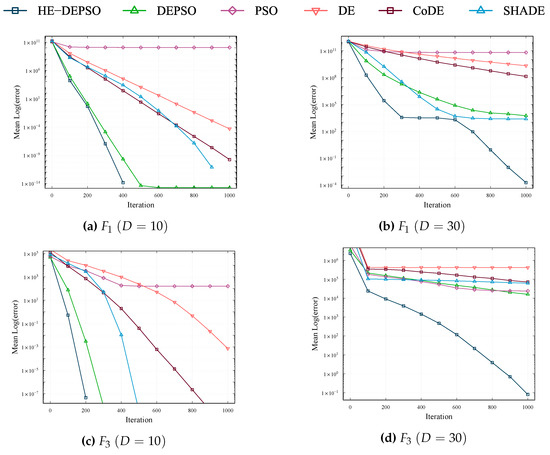
Figure 3. Convergence curves for the functions $F_1$, $F_3$, $F_5$, and $F_8$, with $D=10$ and 30. The horizontal and vertical axis represent the iterations and the mean error values for the 31 independent repetitions.

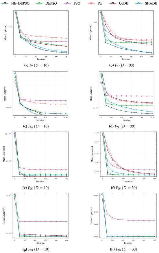
Figure 4. Convergence curves for the functions $F_1$, $F_3$, $F_5$ and $F_8$, with $D=10$ and 30. The horizontal and vertical axis represent the iterations and the mean error values for the 31 independent repetitions.

• The convergence properties of the functions $F_1-F_4$, $F_6$, and $F_9$ can be identified within the same class; this can be observed with the help of Figure 3a–d. In this type, the HE-DEPSO algorithm shows faster convergence than the other algorithms at $D=10$, while at $D=30$ it obtains a better mean error value.
• In Figure 3e–h, the convergence curves of functions $F_5$ and $F_8$ are presented, which are similar to the corresponding ones for functions $F_{10}$, $F_{16}$, $F_{17}$, and $F_{20}$. All algorithms have different degrees of evolutionary stagnation or exhibit slow evolution for these functions.
• The convergence curves of the functions $F_{12}-F_{15}$, $F_{18}-F_{19}$, $F_{23}$, and $F_{29}-F_{30}$ are similar to the curves of the functions $F_7$ and $F_{24}$ (see Figure 4a–d) obtained for the HE-DEPSO algorithm. In this type, HE-DEPSO presents a fast convergence at the beginning and, subsequently, it keeps evolving downward.
• The evolutionary process presented in the convergence curves of the functions $F_{22}$ and $F_{27}$ follows the same trend as the convergence curves of the functions $F_{25}$ and $F_{28}$, as can be seen in Figure 4e–h. Here, most of the algorithms present stagnation in an accelerated way, although some of them manage to keep evolving downward.

The experiments performed above prove the superiority of the proposed HE-DEPSO algorithm in solving different optimization problems. The reasons why the HE-DEPSO algorithm obtains such superior performance can be summarized as follows:

• The adaptive hybrid mutation operator implemented in HE-DEPSO is based on the self-adaptive mutation strategy of the DEPSO algorithm, which has proven to be helpful in tackling several complex optimization problems. On the other hand, the collaborative work between the “DE/current-to-EHE/1” mutation strategy with historical information of the elite individuals and the PSO algorithm strategy generates a good balance between exploration and exploitation at different stages of the evolutionary process.
• The self-adaptive control of the F and $Cr$ parameters adopted from the SHADE algorithm allows the mitigation of parameter sensitivity. In this way, the crossover probability and the scale factor are dynamically adjusted during the evolutionary process at the level of each individual, which can make the proposed algorithm suitable for a wider variety of optimization problems.

6. Four-Zero Texture Model Validation

In order to verify the physical feasibility of the 4-zero texture model, it is essential to find sets of numerical values for the parameters $A_u$, $A_d$, ${\varphi }_1$, and ${\varphi }_2$ that minimize the ${\chi }^2\left(X\right)$ function to a value of less than one (see Equation (16)), and also that the numerical values for all $|V_{ckm}|$ predicted for the 4-zero texture model (evaluated in these sets of values) are in agreement with the experimental data. Firstly, an analysis of the HE-DEPSO algorithm’s behavior when optimizing the ${\chi }^2\left(X\right)$ function will be conducted. The study will assess the algorithm’s optimization, convergence, and stability properties, providing insights into its performance when dealing with the ${\chi }^2$ optimization problem.

6.1. HE-DEPSO Performance in ${\chi }^2$ Optimization

The given optimization problem seeks to minimize the function ${\chi }^2\left(X\right)$ given by Equation (17). The search space is constrained by the possible signs of the parameters ${\eta }_u$ and ${\eta }_d$, as shown in Table 1. The phases ${\varphi }_1$ and ${\varphi }_2$ can take values between 0 and $2\pi$. The ranges of parameters $A_u$ and $A_d$ depend on the signs of ${\eta }_u$ and ${\eta }_d$. Specifically considering case of study 1, $A_u$ can take values in the interval $[m_c,m_t]$, while $A_d$ can take values in the interval $[m_s,m_b]$.

6.1.1. Experiment Configuration

Through an experiment, an evaluation of the performance of the HE-DEPSO algorithm in the optimization of the ${\chi }^2\left(X\right)$ function will be carried out in order to determine its ability to find the global minimum. This study will be carried out in the search space defined in case 1 previously mentioned. The performance of HE-DEPSO will be compared with the PSO and DE algorithms, as well as with advanced variants of the DE algorithm, such as CoDE, SHADE, and DEPSO. To ensure a fair comparison, standard parameters have been set for all algorithms ($tmax=1000$ and $NP=100$) and 31 independent runs have been performed. The settings of the other parameters of each algorithm have been made following the indications in Table 3.

6.1.2. Experiment Results

To evaluate the effectiveness of the proposed HE-DEPSO algorithm, comparisons and analysis of its optimization results were performed with the DE, PSO, and three advanced variants of DE algorithms applied to the ${\chi }^2\left(X\right)$ function. Using an approach similar to that described in Section 5, Table 6 presents the statistical data for each algorithm evaluated.

Table 6. Comparison of results between HE-DEPSO, DE, PSO, and three advanced variants of the DE algorithm on the function ${\chi }^2\left(X\right)$.

Function	Metrics	HE-DEPSO	DEPSO	SHADE	CoDE	DE	PSO
${\chi }^2\left(X\right)$	Mean	1.7267 $\mathbf{\times } {\mathbf{10}}^{\mathbf{-}\mathbf{28}}$	3.4971 $\times {10}^{-28}$	7.2296 $\times {10}^{-3}$	2.3720 $\times {10}^{-5}$	6.1610 $\times {10}^{-13}$	7.4247 $\times {10}^0$
	Std	1.4496 $\mathbf{\times } {\mathbf{10}}^{\mathbf{-}\mathbf{28}}$	5.6400 $\times {10}^{-28}$	8.7102 $\times {10}^{-3}$	7.7748 $\times {10}^{-5}$	3.4294 $\times {10}^{-12}$	1.6815 $\times {10}^1$
	Classification	1	2	5	4	3	6
	Significance		+	+	+	+	+
Final classification		1	2	5	4	3	6
W/T/L		−/−/−	1/0/0	1/0/0	1/0/0	1/0/0	1/0/0

According to the data presented in Table 6, the HE-DEPSO algorithm excels in obtaining the best results in optimizing the ${\chi }^2\left(X\right)$ function, outperforming DEPSO. Although DEPSO comes close to the results of HE-DEPSO, its accuracy is not matched. On the other hand, the DE algorithm also demonstrated acceptable accuracy, although it was lower than that achieved by HE-DEPSO and DEPSO. In contrast, the SHADE, CoDE, and PSO algorithms obtained the lowest results compared to the others. In terms of average ranking, HE-DEPSO is positioned as the leader among all the analyzed algorithms. Furthermore, the results of the Wilcoxon test confirm the superiority of HE-DEPSO over DEPSO, SHADE, CoDE, DE, and PSO in the optimization of the ${\chi }^2\left(X\right)$ function.

Figure 5 presents the curves obtained over 31 independent runs by the HE-DEPSO, DEPSO, SHADE, CoDE, DE, and PSO algorithms. It is observed that the HE-DEPSO algorithm exhibits excellent convergence behavior, consistently outperforming SHADE, CoDE, DE, and PSO and achieving a lower mean error value. Although DEPSO converges faster starting from the 300 iteration, the performance of HE-DEPSO stands out for its consistency and exploration capability, which could explain its more extended convergence compared to DEPSO.

Figure 5. Convergence curves of the error measure in the solution for the ${\chi }^2\left(X\right)$ function. The horizontal and vertical axis represent the iterations and the mean error values for the 31 independent iterations.

In Figure 6, box and whisker plots show the results of the HE-DEPSO, DEPSO, SHADE, CoDE, DE, and PSO algorithms, based on the best overall fits of 31 independent runs to the chi-square function. These graphs illustrate the distribution of these values into quartiles, with the median highlighted by a red horizontal line within a blue box. The box boundaries correspond to the upper (Q3) and lower (Q1) quartiles. Lines extending from the box indicate the maximum and minimum values, excluding outliers represented by the “+” symbol in blue. The green circles represent the mean of the overall best fits of the 31 independent runs.

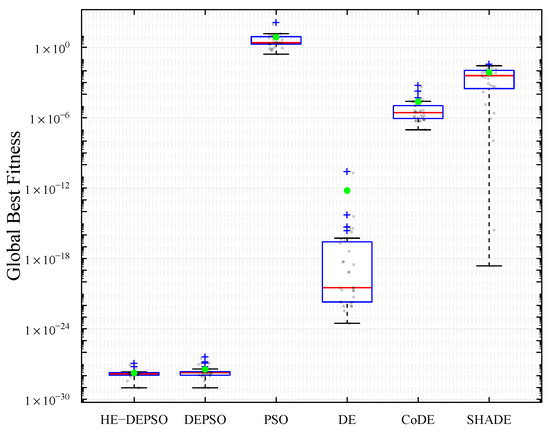
Figure 6. Box and whisker plots of the best global fit values obtained by HE-DEPSO and the DEPSO, SHADE, CoDE, DE, and PSO algorithms in the 31 independent repetitions in the ${\chi }^2\left(X\right)$ function. The horizontal axis shows the algorithms to be compared, and the vertical axis shows the global fit values.

According to the box and whisker plots, the HE-DEPSO algorithm demonstrated superior performance compared with the other evaluated algorithms regarding stability and solution quality, based on 31 independent runs. The distribution of the best global fitness values achieved by HE-DEPSO presents a higher concentration around a lower optimum, reflected in a lower average than the other algorithms. Consequently, the HE-DEPSO offers a more robust and stable performance.

6.2. Valid Regions for Parameters $A_u,A_d,{\varphi }_1$, and ${\varphi }_2$

In this subsection, we present the results obtained after applying the HE-DEPSO algorithm to search for valid regions of the $A_u$, $A_d$, ${\varphi }_1$, and ${\varphi }_2$ parameters. This process was carried out using the most recent experimental values of the $V_{CKM}$ matrix elements, the quark masses, and the Jarlskog invariant (see Appendix A).

Figure 7 and Figure 8 present the allowed regions for the parameters $A_u$, $A_d$, ${\varphi }_1$, and ${\varphi }_2$, scaled as $A_u/m_t,A_d/m_b,{\varphi }_1/\pi$, and ${\varphi }_2/\pi$, respectively, in the first case study of Table 1. These regions are classified by the solutions found using the HE-DEPSO algorithm and are represented by black, blue, and orange dots, which correspond to different levels of precision of the ${\chi }^2\left(X\right)$ function. The orange region, the smallest, indicates the region of highest precision, where experimental data agree best with theoretical predictions. These solutions were found by iteratively executing the algorithm until a total of 5000 solutions were collected at each of the precisions (${\chi }^2<1$, ${\chi }^2<1\times {10}^{-1}$, and ${\chi }^2<1\times {10}^{-2}$).

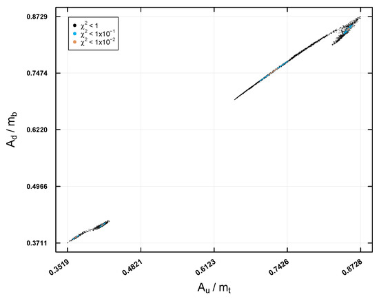
Figure 7. Allowed regions for $A_u$ and $A_d$ constrained based on current experimental data with different levels of precision: ${\chi }^2<1$ (black dots), ${\chi }^2<1\times {10}^{-1}$ (blue dots), and ${\chi }^2<1\times {10}^{-2}$ (orange dots).

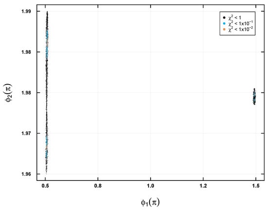
Figure 8. Allowed regions for ${\varphi }_1$ and ${\varphi }_2$ constrained based on current experimental data with different levels of precision: ${\chi }^2<1$ (black dost), ${\chi }^2<1\times {10}^{-1}$ (blue dots), and ${\chi }^2<1\times {10}^{-2}$ (orange dots).

It is worth noting that, for the rest of the case studies (see Table 1), the found regions for the parameters $A_u$, $A_d$, ${\varphi }_1$, and ${\varphi }_2$ were similar.

6.3. Predictions for the $V_{CKM}$ Elements

The second part of model validation is as follows: With the data obtained from the valid regions for the four free parameters of the 4-zero texture model, $A_u$, $A_d$, ${\varphi }_1$, and ${\varphi }_2$, found with the help of HE-DEPSO, we can evaluate the feasibility of the model according to the latest experimental values of the $V_{CKM}$ matrix and the Jarlskog invariant. This can be achieved by checking the model’s predictive power when predicting the remaining elements of the $V_{CKM}$ matrix that were not used within the ${\chi }^2$ fit, i.e., $|V_{cd}|$, $|V_{ud}|$, $|V_{cs}|$, $|V_{tb}|$, $|V_{td}|$, and $|V_{ts}|$. Using Equations (2)–(5), the Chau–Keng parametrization [3], and the solutions found, we can calculate the numerical predictions for those elements. These predictions are then presented using scatter plots. Each graph includes the experimental central value of each element with its associated experimental error value. The points that fall within the region delimited by the experimental values are considered good predictions, while those outside the region are considered poor predictions.

In Figure 9, the predictions for the elements $|V_{ud}|$ and $|V_{cd}|$ in the first case study are presented. The black, blue, and orange points indicate a precision of ${\chi }^2<1$, ${\chi }^2<1\times {10}^{-1}$, and ${\chi }^2<1\times {10}^{-2}$, respectively. For $|V_{cd}|$, the experimental central value $\left(0.22636\right)$ is indicated with a solid red vertical line on the corresponding axis, while its experimental error ($\pm 0.00048$) is shown with two red dashed vertical lines on either side of the central value. In the case of $|V_{ud}|$, the experimental central value $\left(0.97401\right)$ is represented with a solid blue horizontal line on the $|V_{ud}|$ axis, and its experimental error ($\pm 0.00011$) is indicated with two blue dashed horizontal lines on either side of the central value. The predictions for the two elements show that the data with a precision of ${\chi }^2<1$ can be outside the experimental error region, suggesting a poor prediction. On the other hand, the predictions with ${\chi }^2<1\times {10}^{-1}$ and ${\chi }^2<1\times {10}^{-2}$ remain within this region, indicating accurate predictions. This pattern is repeated in the rest of the analyzed case studies.

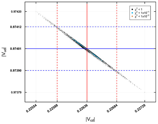
Figure 9. Predictions for $|V_{cd}|$ and $|V_{ud}|$ for ${\eta }_u=+1$ and ${\eta }_d=+1$.

The predictions for the elements $|V_{cs}|$ and $|V_{tb}|$ are shown in Figure 10 for the first case study. The experimental central value of $|V_{cs}|$ is represented by a solid red vertical line at the center of the $|V_{cs}|$ axis at $0.97320$, while its experimental error of $\pm 0.00011$ is indicated by red dashed vertical lines on either side. The experimental central value of $|V_{tb}|$ is shown by a solid blue horizontal line at the center of the $|V_{tb}|$ axis at $0.999172$, and its experimental error of $\pm 0.000024$ is represented by blue dashed horizontal lines on either side. According to the predictions shown in Figure 10, the data obtained with ${\chi }^2<1$ do not represent good predictions, as they are outside the experimental errors. On the other hand, the predictions with ${\chi }^2<1\times {10}^{-1}$ and ${\chi }^2<1\times {10}^{-2}$ remain within the error region, indicating that they are good predictions. This pattern is repeated in the four case studies.

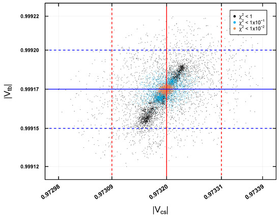
Figure 10. Predictions for $|V_{cs}|$ and $|V_{tb}|$ for ${\eta }_u=+1$ and ${\eta }_d=+1$.

Finally, in Figure 11, the predictions for the elements $|V_{td}|$ and $|V_{ts}|$ are shown in the four case studies. For $|V_{td}|$, the experimental central value is represented by a solid vertical line at $|V_{td}|=0.00854$, and its experimental error with two red dashed vertical lines at $\pm 0.00016$. For $|V_{ts}|$, the experimental central value is shown with a solid blue horizontal line at $|V_{ts}|=0.03978$, and its experimental error with two blue dashed horizontal lines at $\pm 0.00060$. The predictions for these two elements indicate that the data obtained with precisions of ${\chi }^2<1$ and ${\chi }^2<1\times {10}^{-1}$ may be outside the experimental errors, so they are not good predictions. In contrast, the prediction with ${\chi }^2<1\times {10}^{-2}$ remains within the errors, being a good prediction. These characteristics are observed in the four case studies.

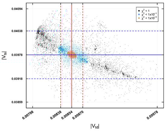
Figure 11. Predictions for $|V_{td}|$ and $|V_{ts}|$ for ${\eta }_u=+1$ and ${\eta }_d=+1$.

When analyzing the predictions of the elements of the $V_{CKM}$ matrix ($|V_{ud}|$, $|V_{cd}|$, $|V_{cs}|$, $|V_{tb}|$, $|V_{td}|$, and $|V_{ts}|$), it was observed that only the solutions of the HE-DEPSO algorithm, with an accuracy of ${\chi }^2<1\times {10}^{-2}$, fit within the limits of experimental error. These solutions are considered valid and capable of reproducing the $V_{CKM}$ matrix in all case studies and elements. Thus, it can be established that the 4-zero texture model is physically viable. It would be interesting, however, to explore the implications of this information obtained within the texture formalism.

7. Conclusions

This paper explored the feasibility of the 4-zero texture model using the most recent experimental values. To gather data that can inform decisions on the model’s viability, we employed a chi-square fit to compare the theoretical expressions of the model with the experimental values of well-measured physical observables. We developed a single-objective optimization model by defining a ${\chi }^2\left(X\right)$ function to identify the allowed regions for the free parameters of the 4-zero texture model that are consistent with the experimental data. To address the challenge of optimizing the ${\chi }^2\left(X\right)$ function within the chi-square fit, we proposed a new DEPSO algorithm variant, HE-DEPSO.

The proposed algorithm has demonstrated its ability to efficiently optimize different functions, particularly those from the CEC 2017 single-objective benchmark functions set. The convergence properties of HE-DEPSO show a good balance between solution precision and convergence speed in most cases. Regarding optimizing the ${\chi }^2\left(X\right)$ function, our findings indicate that HE-DEPSO and DEPSO are more than adequate for solving the optimization problem, with HE-DEPSO providing the best solution quality and consistency. At the same time, DEPSO maintains a faster convergence rate. This part of the investigation also highlights the difficulty that some algorithms can face when optimizing the ${\chi }^2\left(X\right)$ function, such as algorithms like SHADE and CoDE, despite exhibiting good performance on the CEC 2017 test set. We can also conclude that optimization algorithms such as SHADE, CoDE, and DE would be worth considering for optimization problems in high-energy physics. Finally, with the use of the HE-DEPSO algorithm we show that the 4-zero texture model is compatible with current experimental data, and thus we can affirm that this model is physically feasible. Importantly, our proposed approach, with the help of HE-DEPSO, allows a more accurate exploration of the full parameter space of the elements of the 4-zero texture quark mass matrix, an aspect that is often overlooked in analytical approaches. While aligning with the latest experimental data, this approach could enhance the structural features of 4-zero quark mass matrices. It may serve as a valuable starting point for future model building.

Future work will focus on enhancing the convergence speed of the HE-DEPSO algorithm and evaluating its effectiveness across diverse problem domains, exploring its ability to tackle more complex optimization challenges. An extended comparative analysis against other bio-inspired algorithms or other advanced DE variants could also be conducted. Furthermore, this research could be expanded by analyzing additional texture models like 2- and 5-zero texture models and determining their validity based on current experimental data. Additionally, the use of this method could have potential applications in any phenomenological fermion mass model SM extension, for example, nearest-neighbor textures [59], neutrino mass models [60], and discrete flavor symmetries models [14,15].

References

- Battaglia, M.; Buras, A.J.; Gambino, P.; Stocchi, A.; Abbaneo, D.; Ali, A.; Amaral, P.; Andreev, V.; Artuso, M.; Barberio, E.; et al. The CKM Matrix and the Unitarity Triangle. In Proceedings of the First Workshop on the CKM Unitarity Triangle, CERN, Geneva, Switzerland, 13–16 February 2002. [Google Scholar] [CrossRef]
- Fleischer, R. Flavor physics and CP violation. In Proceedings of the European School on High-Energy Physics, Tsakhkadzor, Armenia, 24 August–6 September 2003; pp. 81–150. [Google Scholar]
- Branco, G.C.; Lavoura, L.; Silva, J.P. CP Violation; Clarendon Press: Oxford, UK, 1999; Volume 103. [Google Scholar]
- Altarelli, G.; Feruglio, F. Neutrino masses and mixings: A theoretical perspective. Phys. Rept. 1999, 320, 295–318. [Google Scholar] [CrossRef][Green Version]
- Altarelli, G.; Feruglio, F. Models of neutrino masses and mixings. New J. Phys. 2004, 6, 106. [Google Scholar] [CrossRef]
- Fritzsch, H.; Xing, Z.Z. Mass and flavor mixing schemes of quarks and leptons. Prog. Part. Nucl. Phys. 2000, 45, 1–81. [Google Scholar] [CrossRef]
- Xing, Z.Z. Flavor structures of charged fermions and massive neutrinos. Phys. Rept. 2020, 854, 1–147. [Google Scholar] [CrossRef]
- Gupta, M.; Ahuja, G. Flavor mixings and textures of the fermion mass matrices. Int. J. Mod. Phys. A 2012, 27, 1230033. [Google Scholar] [CrossRef]
- Froggatt, C.D.; Nielsen, H.B. Hierarchy of Quark Masses, Cabibbo Angles and CP Violation. Nucl. Phys. B 1979, 147, 277–298. [Google Scholar] [CrossRef]
- King, S.F.; Luhn, C. Neutrino Mass and Mixing with Discrete Symmetry. Rept. Prog. Phys. 2013, 76, 056201. [Google Scholar] [CrossRef]
- Borzumati, F.; Nomura, Y. Low scale seesaw mechanisms for light neutrinos. Phys. Rev. D 2001, 64, 053005. [Google Scholar] [CrossRef]
- Lindner, M.; Ohlsson, T.; Seidl, G. Seesaw mechanisms for Dirac and Majorana neutrino masses. Phys. Rev. D 2002, 65, 053014. [Google Scholar] [CrossRef]
- Flieger, W.; Gluza, J. General neutrino mass spectrum and mixing properties in seesaw mechanisms. Chin. Phys. C 2021, 45, 023106. [Google Scholar] [CrossRef]
- Aranda, A.; Bonilla, C.; Rojas, A.D. Neutrino masses generation in a Z4 model. Phys. Rev. D 2012, 85, 036004. [Google Scholar] [CrossRef]
- Ahn, Y.H.; Kang, S.K. Non-zero θ13 and CP violation in a model with A4 flavor symmetry. Phys. Rev. D 2012, 86, 093003. [Google Scholar] [CrossRef]
- Sinha, R.; Samanta, R.; Ghosal, A. Maximal Zero Textures in Linear and Inverse Seesaw. Phys. Lett. B 2016, 759, 206–213. [Google Scholar] [CrossRef][Green Version]
- Fritzsch, H. Calculating the Cabibbo angle. Phys. Lett. B 1977, 70, 436–440. [Google Scholar] [CrossRef]
- Fritzsch, H.; Xing, Z.Z. Four zero texture of Hermitian quark mass matrices and current experimental tests. Phys. Lett. B 2003, 555, 63–70. [Google Scholar] [CrossRef]
- Kang, K.; Kang, S.K. New class of quark mass matrix and calculability of the flavor mixing matrix. Phys. Rev. D 1997, 56, 1511–1514. [Google Scholar] [CrossRef]
- Xing, Z.-Z.; Zhao, Z.-H. On the four-zero texture of quark mass matrices and its stability. Nucl. Phys. B 2015, 897, 302–325. [Google Scholar] [CrossRef]
- Gómez-Ávila, S.; López-Lozano, L.; Miranda-Romagnoli, P.; Noriega-Papaqui, R.; Lagos-Eulogio, P. 2-zeroes texture and the Universal Texture Constraint. arXiv 2021, arXiv:2105.01554. [Google Scholar]
- Tani, L.; Rand, D.; Veelken, C.; Kadastik, M. Evolutionary algorithms for hyperparameter optimization in machine learning for application in high energy physics. Eur. Phys. J. C 2021, 81, 170. [Google Scholar] [CrossRef]
- Zhang, Y.; Zhou, D. Application of differential evolution algorithm in future collider optimization. In Proceedings of the 7th International Particle Accelerator Conference (IPAC’16), Busan, Republic of Korea, 8–13 May 2016; pp. 1025–1027. [Google Scholar]
- Wu, J.; Zhang, Y.; Qin, Q.; Wang, Y.; Yu, C.; Zhou, D. Dynamic aperture optimization with diffusion map analysis at CEPC using differential evolution algorithm. Nucl. Instruments Methods Phys. Res. Sect. A Accel. Spectrometers Detect. Assoc. Equip. 2020, 959, 163517. [Google Scholar] [CrossRef]
- Allanach, B.C.; Grellscheid, D.; Quevedo, F. Genetic algorithms and experimental discrimination of SUSY models. J. High Energy Phys. 2004, 2004, 069. [Google Scholar] [CrossRef]
- Bilal; Pant, M.; Zaheer, H.; Garcia-Hernandez, L.; Abraham, A. Differential Evolution: A review of more than two decades of research. Eng. Appl. Artif. Intell. 2020, 90, 103479. [Google Scholar] [CrossRef]
- Ahmad, M.F.; Isa, N.A.M.; Lim, W.H.; Ang, K.M. Differential evolution: A recent review based on state-of-the-art works. Alex. Eng. J. 2022, 61, 3831–3872. [Google Scholar] [CrossRef]
- Pan, J.S.; Liu, N.; Chu, S.C. A Hybrid Differential Evolution Algorithm and Its Application in Unmanned Combat Aerial Vehicle Path Planning. IEEE Access 2020, 8, 17691–17712. [Google Scholar] [CrossRef]
- Opara, K.R.; Arabas, J. Differential Evolution: A survey of theoretical analyses. Swarm Evol. Comput. 2019, 44, 546–558. [Google Scholar] [CrossRef]
- Wang, Y.; Cai, Z.; Zhang, Q. Differential Evolution With Composite Trial Vector Generation Strategies and Control Parameters. IEEE Trans. Evol. Comput. 2011, 15, 55–66. [Google Scholar] [CrossRef]
- Peñuñuri, F.; Cab, C.; Carvente, O.; Zambrano-Arjona, M.; Tapia, J. A study of the Classical Differential Evolution control parameters. Swarm Evol. Comput. 2016, 26, 86–96. [Google Scholar] [CrossRef]
- Tanabe, R.; Fukunaga, A. Success-history based parameter adaptation for Differential Evolution. In Proceedings of the 2013 IEEE Congress on Evolutionary Computation, Cancun, Mexico, 20–23 June 2013; pp. 71–78. [Google Scholar] [CrossRef]
- Qin, A.K.; Huang, V.L.; Suganthan, P.N. Differential Evolution Algorithm with Strategy Adaptation for Global Numerical Optimization. IEEE Trans. Evol. Comput. 2009, 13, 398–417. [Google Scholar] [CrossRef]
- Das, S.; Abraham, A.; Chakraborty, U.K.; Konar, A. Differential Evolution Using a Neighborhood-Based Mutation Operator. IEEE Trans. Evol. Comput. 2009, 13, 526–553. [Google Scholar] [CrossRef]
- Rahnamayan, S.; Tizhoosh, H.R.; Salama, M.M. Opposition-based differential evolution. IEEE Trans. Evol. Comput. 2008, 12, 64–79. [Google Scholar] [CrossRef]
- Zhang, J.; Sanderson, A. JADE: Adaptive Differential Evolution with Optional External Archive. Evol. Comput. IEEE Trans. 2009, 13, 945–958. [Google Scholar] [CrossRef]
- Chakraborty, S.; Saha, A.K.; Sharma, S.; Sahoo, S.K.; Pal, G. Comparative Performance Analysis of Differential Evolution Variants on Engineering Design Problems. J. Bionic Eng. 2022, 19, 1140–1160. [Google Scholar] [CrossRef] [PubMed]
- Lagos-Eulogio, P.; Miranda-Romagnoli, P.; Seck-Tuoh-Mora, J.C.; Hernández-Romero, N. Improvement in Sizing Constrained Analog IC via Ts-CPD Algorithm. Computation 2023, 11, 230. [Google Scholar] [CrossRef]
- Wang, S.; Li, Y.; Yang, H. Self-adaptive mutation differential evolution algorithm based on particle swarm optimization. Appl. Soft Comput. 2019, 81, 105496. [Google Scholar] [CrossRef]
- Novaes, S.F. Standard model: An Introduction. In Proceedings of the 10th Jorge Andre Swieca Summer School: Particle and Fields, São Paulo, Brazil, 6–12 February 1999; pp. 5–102. [Google Scholar]
- Langacker, P. Introduction to the Standard Model and Electroweak Physics. In Proceedings of the Theoretical Advanced Study Institute in Elementary Particle Physics: The Dawn of the LHC Era, Boulder, CO, USA, 1 January 2010; pp. 3–48. [Google Scholar] [CrossRef]
- Isidori, G.; Nir, Y.; Perez, G. Flavor Physics Constraints for Physics Beyond the Standard Model. Ann. Rev. Nucl. Part. Sci. 2010, 60, 355. [Google Scholar] [CrossRef]
- Antonelli, M.; Asner, D.M.; Bauer, D.; Becher, T.; Beneke, M.; Bevan, A.J.; Blanke, M.; Bloise, C.; Bona, M.; Bondar, A.; et al. Flavor Physics in the Quark Sector. Phys. Rept. 2010, 494, 197–414. [Google Scholar] [CrossRef]
- Eidelman, S. Review of particle physics. Particle Data Group. Phys. Lett. B 2004, 592, 1. [Google Scholar] [CrossRef]
- Félix-Beltrán, O.; González-Canales, F.; Hernández-Sánchez, J.; Moretti, S.; Noriega-Papaqui, R.; Rosado, A. Analysis of the quark sector in the 2HDM with a four-zero Yukawa texture using the most recent data on the CKM matrix. Phys. Lett. B 2015, 742, 347–352. [Google Scholar] [CrossRef]
- Barranco, J.; Delepine, D.; Lopez-Lozano, L. Neutrino mass determination from a four-zero texture mass matrix. Phys. Rev. D 2012, 86, 053012. [Google Scholar] [CrossRef]
- Eberhart, R.C.; Kennedy, J. A new optimizer using particle swarm theory. In Proceedings of the MHS’95, Proceedings of the Sixth International Symposium on Micro Machine and Human Science, Nagoya, Japan, 4–6 October 1995; pp. 39–43. [Google Scholar]
- Shi, Y.; Eberhart, R. A modified particle swarm optimizer. In Proceedings of the 1998 IEEE International Conference on Evolutionary Computation Proceedings, IEEE World Congress on Computational Intelligence (Cat. No. 98TH8360), Anchorage, Alaska, 4–9 May 1998; pp. 69–73. [Google Scholar] [CrossRef]
- Storn, R.; Price, K. Differential Evolution: A Simple and Efficient Adaptive Scheme for Global Optimization Over Continuous Spaces. J. Glob. Optim. 1995, 23. Available online: https://cse.engineering.nyu.edu/~mleung/CS909/s04/Storn95-012.pdf (accessed on 1 July 2024).
- Storn, R.; Price, K. Differential Evolution—A Simple and Efficient Heuristic for Global Optimization over Continuous Spaces. J. Glob. Optim. 1997, 11, 341–359. [Google Scholar] [CrossRef]
- Sánchez Vargas, O.; De León Aldaco, S.E.; Aguayo Alquicira, J.; Vela Valdés, L.G.; Mina Antonio, J.D. Differential Evolution Applied to a Multilevel Inverter—A Case Study. Appl. Sci. 2022, 12, 9910. [Google Scholar] [CrossRef]
- Batool, R.; Bibi, N.; Muhammad, N.; Alhazmi, S. Detection of Primary User Emulation Attack Using the Differential Evolution Algorithm in Cognitive Radio Networks. Appl. Sci. 2023, 13, 571. [Google Scholar] [CrossRef]
- Elsayed, S.M.; Sarker, R.A.; Ray, T. Differential evolution with automatic parameter configuration for solving the CEC2013 competition on Real-Parameter Optimization. In Proceedings of the 2013 IEEE Congress on Evolutionary Computation, Cancun, Mexico, 20–23 June 2013; pp. 1932–1937. [Google Scholar] [CrossRef]
- Zhong, X.; Cheng, P. An elite-guided hierarchical differential evolution algorithm. Appl. Intell. 2021, 51, 4962–4983. [Google Scholar] [CrossRef]
- Yang, Q.; Guo, X.; Gao, X.D.; Xu, D.D.; Lu, Z.Y. Differential Elite Learning Particle Swarm Optimization for Global Numerical Optimization. Mathematics 2022, 10, 1261. [Google Scholar] [CrossRef]
- Huang, Y.; Yu, Y.; Guo, J.; Wu, Y. Self-adaptive Artificial Bee Colony with a Candidate Strategy Pool. Appl. Sci. 2023, 13, 10445. [Google Scholar] [CrossRef]
- Wang, S.; Li, Y.; Yang, H.; Liu, H. Self-adaptive differential evolution algorithm with improved mutation strategy. Soft Comput. 2017, 22, 3433–3447. [Google Scholar] [CrossRef]
- Kumar, A.; Price, K.V.; Mohamed, A.W.; Hadi, A.A.; Suganthan, P.N. Problem Definitions and Evaluation Criteria for the CEC 2017 Special Session and Competition on Single Objective Bound Constrained Numerical Optimization; Technical Report; Nanyang Technological University: Singapore, 2016; pp. 1–34. [Google Scholar]
- Branco, G.C.; Emmanuel-Costa, D.; Simoes, C. Nearest-Neighbour Interaction from an Abelian Symmetry and Deviations from Hermiticity. Phys. Lett. B 2010, 690, 62–67. [Google Scholar] [CrossRef]
- Centelles Chuliá, S.; Herrero-Brocal, A.; Vicente, A. The Type-I Seesaw family. J. High Energy Phys. 2024, 2024, 60. [Google Scholar] [CrossRef]
- Fritzsch, H.; Xing, Z.Z.; Zhang, D. Correlations between quark mass and flavor mixing hierarchies. Nucl. Phys. B 2022, 974, 115634. [Google Scholar] [CrossRef]
Disclaimer/Publisher’s Note: The statements, opinions and data contained in all publications are solely those of the individual author(s) and contributor(s) and not of MDPI and/or the editor(s). MDPI and/or the editor(s) disclaim responsibility for any injury to people or property resulting from any ideas, methods, instructions or products referred to in the content. |
© 2024 by the authors. Licensee MDPI, Basel, Switzerland. This article is an open access article distributed under the terms and conditions of the Creative Commons Attribution (CC BY) license (https://creativecommons.org/licenses/by/4.0/).