Efficient Implementation of Multilayer Perceptrons: Reducing Execution Time and Memory Consumption

Abstract

A technique is presented that reduces the required memory of neural networks through improving weight storage. In contrast to traditional methods, which have an exponential memory overhead with the increase in network size, the proposed method stores only the number of connections between neurons. The proposed method is evaluated on feedforward networks and demonstrates memory saving capabilities of up to almost 80% while also being more efficient, especially with larger architectures.

1. Introduction

Artificial neural network (ANN) is an established machine learning technique that is widely used due to the flexibility it provides. Several problems have been solved using ANNs and they are currently used in different commercial products [1]. Researchers have been interested in creating different types of ANNs to solve specific problems [2]. In the present work, no new type of network is proposed. Instead, a very versatile type of network has been selected and a new way of implementation is proposed for its use. This type of network is known as a multilayer perceptron (MLP), where the processing elements (PEs) are fully connected to all the PEs of the following layer [3]. MLP is one of the most employed models in neural network applications, where its main characteristic is the use of the backpropagation training algorithm, and achieving an implementation that may reduce execution times and memory consumption when using such an algorithm [4,5]. Figure 1 shows an example of MLP.

Figure 1. Graphic representation of an MLP. It can be observed that in its architecture, it has an input layer formed by neurons 0 to 3, another hidden layer with neurons 4, 5 and 6, and finally, the last layer, the output layer is formed by neurons 7 and 8. It can be observed that each neuron of a layer is connected with all the neurons of the next layer.

This work focuses mainly on the connectivity of the network, known as weights, since it is the most performance-consuming part of the network. The conventional way of storing the weights of a network is by using a two-dimensional array, such as the one displayed in Figure 2a. The reason why this method has been used is because the array indexes map the network connections. That is, the position i,j of the array indicates the connection $w_{ij}$ that goes from neuron i to neuron j, bearing resemblance to what is known as a sparse matrix [6].

Figure 2. Different ways of storing the weights of a network. Specifically, the example network in Figure 1 is being represented. The gray boxes indicate positions that occupy memory but have no relevant value; the blue boxes represent connections from the first layer to the second layer, while the orange boxes are the connections of neurons from the second layer to the last layer. (a) The traditional way in which the weights of a network are stored by using a two-dimensional array. (b) Storing the weights of the network in an upper triangular array. (c) Proposed way of storing the network weights, where they are all stored consecutively.

However, as can be seen in Figure 2a, the network connections do not occupy the entire matrix and are not dispersed. It can be seen that they follow a pattern and that small submatrices are formed. The proposed method (Figure 2c) will save solely these submatrices despite saving the general matrix. One of the challenges we face regarding the indexing of submatrices is finding the proper method, but this is solved by generating new indexes from a function.

The reason for focusing on network connectivity lies in Amdahl’s Law, which states that the best option for improving a system is the one that has the greatest impact [7]. Thus, this paper proposes a method to reduce the memory needed to store a network by focusing on the connectivity of an MLP.

To conclude, after demonstrating the saving of the used memory by the proposed method to store the network information, it is shown that this method does not negatively affect the speed at which the network runs, in fact, the proposed method improves performance by making the ANN run even faster.

2. Materials and Methods

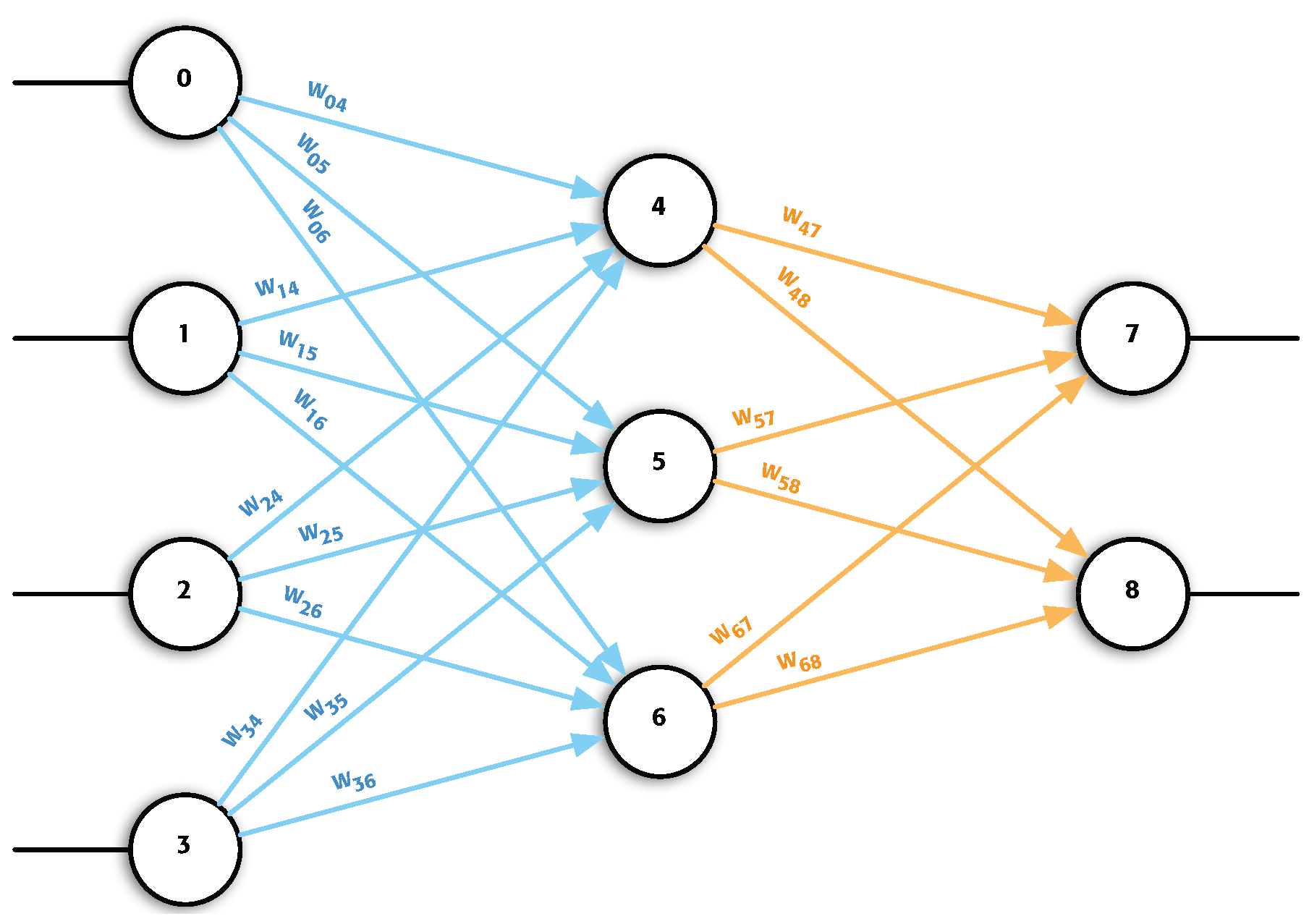
2.1. Proposed Approach

In the event of saving the neural network configuration, it is necessary to emphasize how to store the weights of the connections, because this is what occupies most space and the other data hardly take up any [8]. The first option we find is to save the weights in a square matrix where one of the dimensions would be the input neurons and the other the output dimensions. With this technique, we can keep all the weights without any problem, the only thing we have are several positions that are at zero, pointing out that there are no connections between them.

A way of not consuming so much memory would be to eliminate those values that are useless. By not storing values that are never actually used, we will manage to avoid having so many cache failures and we will be able to take better advantage of the location of the data [9,10]. To achieve this, we can look at the literature where we would find out that this is an issue that occurs sometimes, and the matrices with values which do not serve us are called the sparse matrix [11]. What is performed with this is to eliminate all the positions that do not work for us by storing the matrix otherwise. Although there are different implementations of using the sparse matrix, all of them have something in common, that is, they are only profitable to use if you have a lot of unusable values and massive data. Generally, useful data should be around 10% at most, and you should have several thousands of records. If we analyze the weight matrices of our neural networks, the weights occupy approximately 30% of the total matrix, and we also do not meet the condition of several thousands of records since we are not close to that number. This fact will be discussed in detail in later sections.

We should therefore analyze the feedforward networks, as, like it says in the literature, these networks can be stored in an upper triangular matrix, as shown in Figure 2b [12,13].

Through this, an important memory saving method is achieved, since half of the storage is used, with the triangular matrix, although there are still many values that are not employed. This is due to the fact that the connectivity of an MLP is feedforward from layer to layer, implying that those neurons that are in the same layer, or more than one layer away, will not be linked by a weight.

Furthermore, if we look at how these networks are stored, it is possible to observe that they follow a common pattern (see Figure 2). These are collected in small subarrays, which are defined by the PEs in one layer and in the next. Since it is feasible to know how many weights each of these networks has, we can store these submatrices, a method which is based on the present paper.

As described above, the proposed solution will involve storing only the values that are useful in an array. If, for instance, we use a network with 4 neurons in the input layer, 2 in the output layer and 3 in the only hidden layer, as per the example in Figure 2, it is shown how much memory is used to store the network. In Table 1, it is also possible to see how much space is used.

Table 1. Amount of memory used to store the weights of the different approximations used in Figure 2.

Approach	Cells	Saving
Matrix	81	-
Superior triangular matrix	45	44.4%
Proposed approach	18	77.7%

2.2. Implementation

In the previous section, the proposed solution stores all the weights consecutively, but one very important thing is lost, i.e., the matrix indices, which serve to reference the positions of the weights in the neural network. In order to know which position of the array of weights is related to the weight in the network, some additional information needs to be stored. This section explains how the entire neural network is held in memory.

2.2.1. Required Variables

• num_layer: Number of layers in the network (including input, output and hidden layers).
• num_neurons: Number of neurons in the network.
• Layer (array): The i position indicates the number of processing elements in the i layer.
• Position (array): This indicates which layer the processing element i belongs to.
• Index (array): This indicates the position that the processing element occupies within the layer.
• num_weights: Number of weights that the network has.
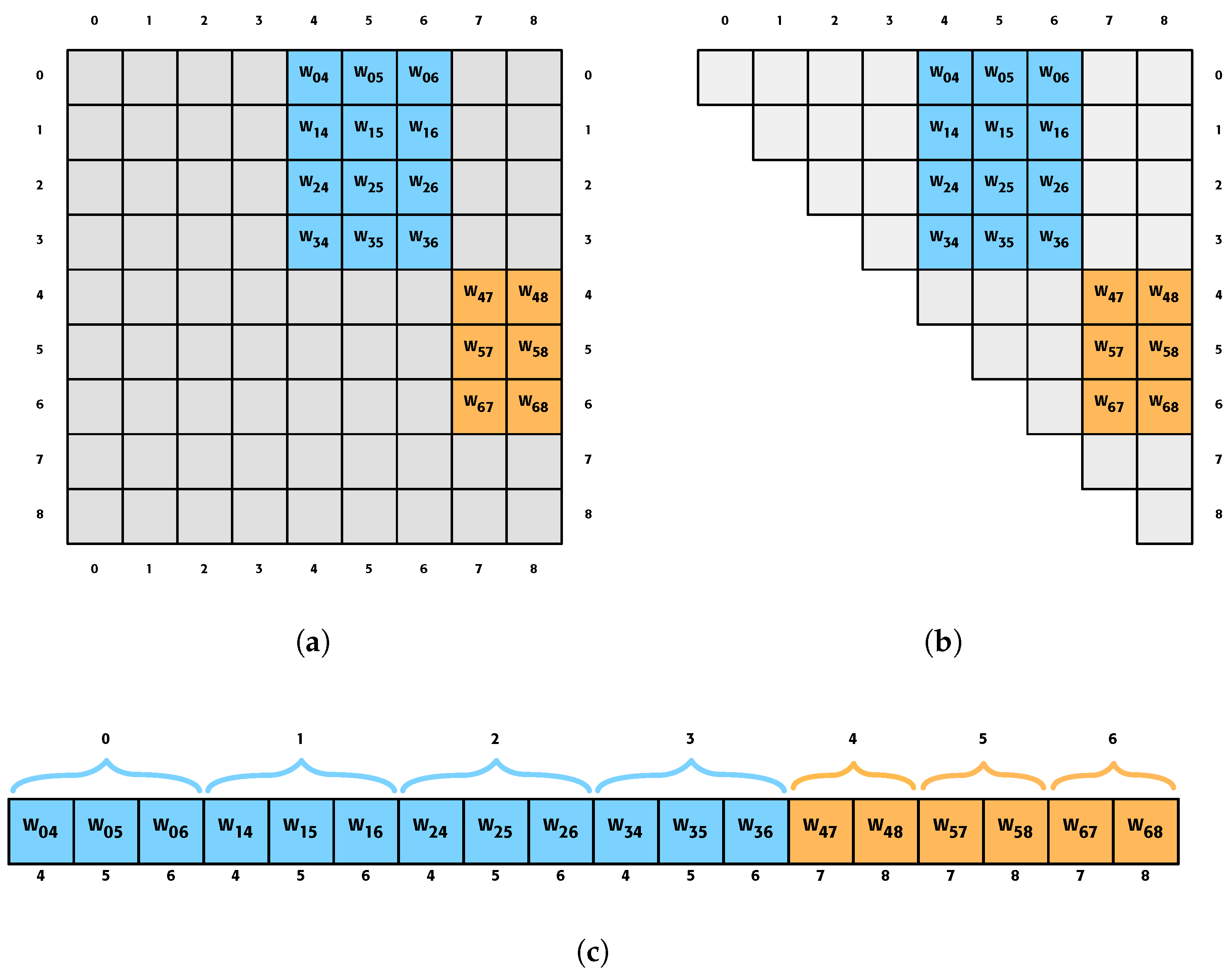
• Weight (array): Value of the network connections.
• Stride (array): The i position indicates where the outgoing weights of the i neuron start.

2.2.2. Length of Arrays

• Layer: The size of this array is given by the value of num_layer, that is, the number of layers.
• Index and position: The size of this array is given by the value of num_neurons, that is, the number of neurons in the network.
• Stride: The size of this array is given by the number of neurons that have outgoing connections, i.e., all the neurons except the output layer.

  $$size\left(stride\right)=num\_neurons-layer[num\_layer-1]$$

  (1)
• Weight: The size of this array is determined by the number of outgoing connections that can exist, which is determined by the num_weight variable:

  $$num\_weights=\sum _{i=0}^{num\_layers-1}layer\left[i\right]\ast layer[i+1]$$

  (2)

Once we have gathered all the necessary information, we still need to know how to access a weight by referencing it with the input and output neurons. We can perform this using the formula below:

$$w_{ij}=weight[stride\left[i\right]+index\left[j\right]]$$

(3)

Figure 3 shows the values of the different arrays used in the proposed method for a neural network.

Figure 3. Array values using the proposed method for the example in Figure 1. The index of the arrays “index” and “position” and “stride” refer to the number of neurons to which it refers. The values of the “index” array indicate the position that a neuron occupies within a layer. The array “position” values indicate the layer number to which a neuron belongs. The array “weights” values are the values of the network connections. The “stride” values indicate at which position in the array weight the outgoing weights of a neuron start.

Finally, it remains to be checked if all this auxiliary information that we added improves the memory consumption used in the code. To know the amount that is consumed, they are used in the equations shown below (the sizeof(int) and sizeof(float) simply imply the value of the size of an integer and a float, respectively):

$$\begin{array}{cc}\hfill Traditional=& (2+num\_neurons)\ast sizeof\left(int\right)\hfill \\ \hfill & +num\_neuron{s}^2\ast sizeof\left(float\right)\hfill \end{array}$$

(4)

$$\begin{array}{cc}\hfill Proposed=& (3+3\ast num\_neurons+num\_layers+\hfill \\ \hfill & layer[num\_layers-1])\ast sizeof(int)\hfill \\ \hfill & +num\_weights\ast sizeof\left(float\right)\hfill \end{array}$$

(5)

In light of these equations, the comparative calculation to estimate the difference in consumption between the traditional and the proposed method is not a trivial issue. While in the former it is only necessary to know the number of neurons ($num\_neurons$), our method incorporates another series of variables that depend directly on the architecture of the MLP network under analysis.

2.2.3. Pseudocode

The pseudocode of the proposed solution is shown in Listing 1. It is important to highlight that the variables NUM_NEURONS and NUM_LAYERS are predefined by the network to be simulated, while getArrayInt is a function that returns an array of integers of the size indicated by the parameter.

Listing 1. Pseudocode of the proposed solution.

POSITION =  getArrayInt (NUM_NEURONS); INDEX       =  getArrayInt (NUM_NEURONS);  for (l = i = 0; i < NUM_LAYERS; i++) {    for (j = 0; j < LAYER[i]; j++, l++) {      POSITION[l] = i;      INDEX[l] = j;    }  } TMP = NUM_NEURONS − LAYER[NUM_LAYERS − 1]; STRIDE =  getArrayInt (TMP); STRIDE[0] = 0;  for (i = 1; i < TMP; i++) {    STRIDE[i] = STRIDE[i − 1] +                          LAYER[POSITION[i − 1] + 1];  } NUM_WEIGHTS = 0;  for (i = 0; i < NUM_LAYERS − 1; i++) {    NUM_WEIGHT += LAYER[i] ∗ LAYER[i + 1];  }

Listing 2 shows how the output of the network would be obtained. The NET is an array that stores the output of each neuron, while ACTIVATION is an array containing the activation functions of each neuron.

Listing 2. Pseudocode to obtain the output network.

first_pe = in_pe = 0; for (l = 1; l < NUM_LAYERS; l++) {   first_pe += LAYER[l − 1];   for (in = 0; in < LAYER[l − 1];          in++, in_pe++) {     pe = first_pe;     for (out = 0; out < LAYER[l];            out++, pe++) {       NET[pe] += NET[pe] ∗                            WEIGHT[out+STRIDE[in_pe]];     }   }   for (tmp = first_pe; tmp < pe; tmp++) {     NET[tmp] = ACTIVATION[tmp](NET[TMP]);   } }

3. Results

It is important to emphasize that the proposed method does not look to improve the network results, i.e., it does not obtain better metrics in accuracy, F1 score or others [14]. The proposed method aims to reduce the memory consumption needed to store a network.

We have tested the method described for networks whose structures are designed to solve the problems found in the UCI repository, specifically for iris [15], cancer [16] and ionosphere [17]. The networks that have been tested have 1, 2 and 3 hidden layers for all three problems. The network structures used can be seen in Table 2. These datasets have been chosen since they are classical problems used in classification problems, based on MLP structures used in previous works, and which have been found to achieve good performance [18].

Table 2. Topology of the networks used for the experimental results. The numbers indicate the amount of neurons on each layer. The first and last values represent the input and output layers, respectively, and the middle numbers are the hidden layers.

Dataset	One Hidden Layer	Two Hidden Layers	Three Hidden Layers
Iris	4, 5, 3	4, 5, 7, 3	4, 4, 5, 5, 3
Cancer	9, 7, 1	9, 7, 3, 1	9, 12, 8, 4, 1
Ionosphere	34, 9, 1	34, 9, 4, 1	34, 12, 8, 4, 1

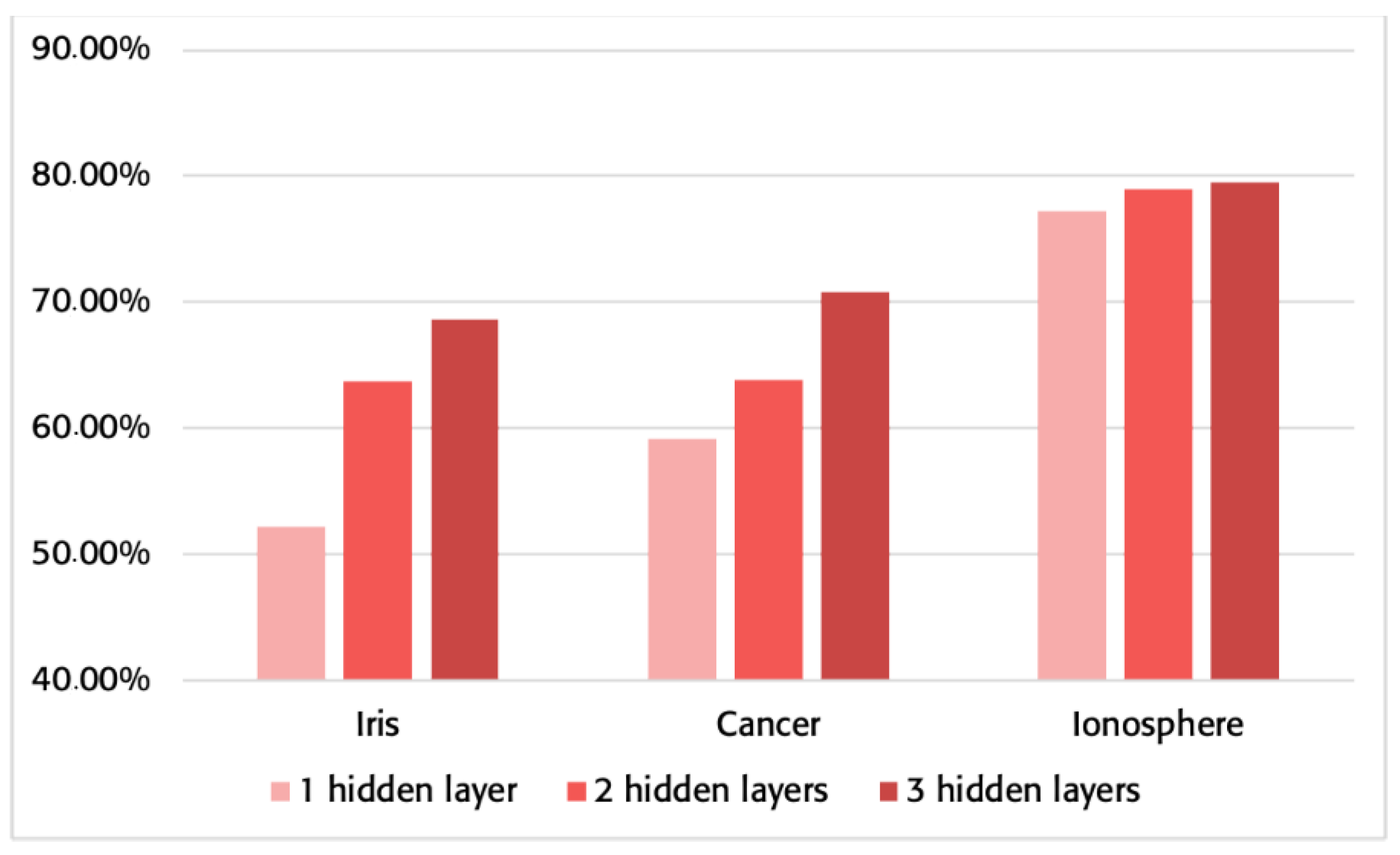
3.1. Memory Consumption

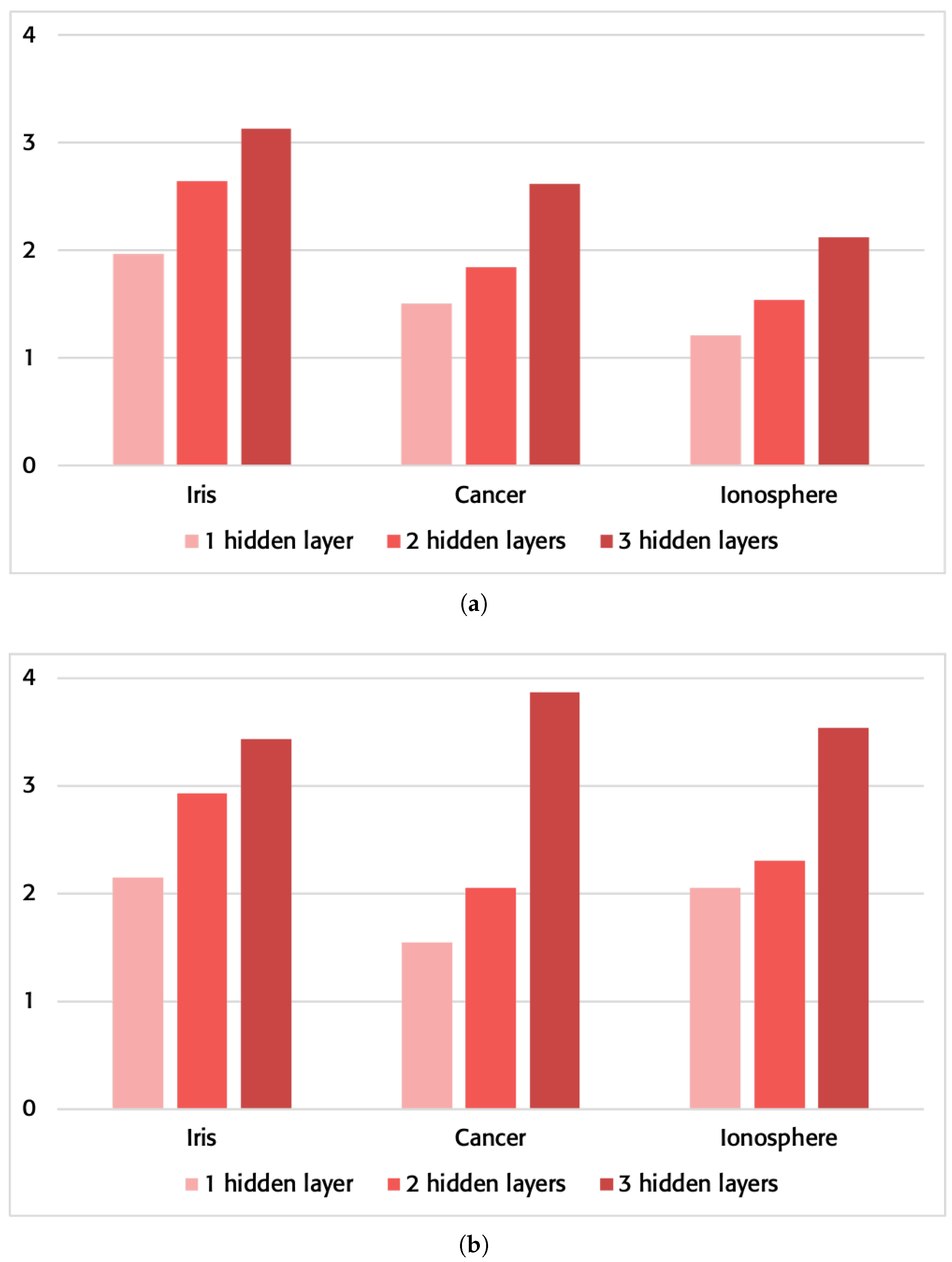
The algorithm presented in this work has a different memory consumption than the traditional method. Next, you can see in Figure 4 the memory saving process when using the proposed method against the traditional one. In addition, Table 3 shows the memory used for all the cases employed.

Figure 4. Percentage of saved memory using the proposed method instead of the traditional one for the networks specified in Table 2.

Table 3. Memory in bytes used to store ANNs. The second column indicates the topology of the network. The third and fourth columns represent the memory used in bytes to store the network using the traditional and proposed methods, respectively. The last column indicates the amount of memory saved by using the proposed method instead of the traditional method.

Dataset	Network Topology	Traditional Approach	Proposed Approach	Memory Saving
Iris	4, 5, 3	644 B	308 B	52.17%
	4, 5, 7, 3	1544 B	560 B	63.73%
	4, 4, 5, 5, 3	1876 B	588 B	68.66%
Cancer	9, 7, 1	1244 B	508 B	59.16%
	9, 7, 3, 1	1704 B	616 B	63.85%
	9, 12, 8, 4, 1	4788 B	1400 B	70.76%
Ionosphere	34, 9, 1	7940 B	1812 B	77.18%
	34, 9, 4, 1	9432 B	1988 B	78.92%
	34, 12, 8, 4, 1	14188 B	2900 B	79.56%

The minimum improvement in memory consumption is over 50%, although most comparisons range from over 60% to almost 80%. This significant improvement in the bytes required for storing the network structure and weights shows a clear significance that is especially beneficial as the MLP grows in complexity.

3.2. Operation Time

Achieving such a noticeable improvement when storing a network is a great accomplishment, but it is necessary to check how it affects the speed of execution. This is necessary since the scenario where the proposed method can be used may vary depending on the performance of the system.

With the aim of achieving representative and reliable results, all the networks run a million patterns to measure the time. The way we have measured the times has been to run each test 10 times and then use the average of those runs as a result. Furthermore, in order to avoid equipment bias, times are taken both on a laptop and on a server, in addition to measuring the times with and without using the optimization options [19,20].

3.2.1. Personal Computer

All tests were conducted on a 2017 macbook pro with i5-7360U CPU @ 2.30 GHz (Apple, Cupertino, CA, USA) and with the clang compiler in the clang-900.0.39.2 version [21].

These first times have been taken without using any of the optimization options provided by the compiler. The results can be checked in Table 4, and Figure 5 shows the increased speed. The reduction in time can be observed in all tested runs, showing a pattern of our proposed model of performance improvement at a higher network complexity.

Table 4. Performance in network execution on a personal computer without using compiler optimization flags and using “-O3-ffast-math-funroll-loops-ftree-vectorize-march=native”.

		No Optimization Flags			Using Optimization Flags
	Network Topology	Traditional Approach	Proposed Approach	Speed Up	Traditional Approach	Proposed Approach	Speed Up
Iris	4, 5, 3	0.4108 s	0.2084 s	1.9712x	0.1295 s	0.0604 s	2.1440x ↑
	4, 5, 7, 3	1.1077 s	0.4185 s	2.6468x	0.3152 s	0.1075 s	2.9320x ↑
	4, 4, 5, 5, 3	1.3989 s	0.4470 s	3.1295x	0.3942 s	0.1147 s	3.4367x ↑
Cancer	9, 7, 1	0.5568 s	0.3690 s	1.5089x	0.1459 s	0.0942 s	1.5488x ↑
	9, 7, 3, 1	0.8677 s	0.4695 s	1.8481x	0.2295 s	0.1117 s	2.0546x ↑
	9, 12, 8, 4, 1	2.9614 s	1.1292 s	2.6225x	0.8527 s	0.2204 s	3.8688x ↑
Iono…	34, 9, 1	1.6810 s	1.3907 s	1.2087x	0.5276 s	0.2569 s	2.0537x ↑
	34, 9, 4, 1	2.3799 s	1.5479 s	1.5375x	0.6511 s	0.2823 s	2.3064x ↑
	34, 12, 8, 4, 1	4.9259 s	2.3174 s	2.1256x	1.4572 s	0.4120 s	3.5368x ↑

Figure 5. Sped-up improvement of the proposed method vs. the traditional method in network execution on a personal computer. (a) Without using the compiler optimization flags. (b) Using the compiler optimization flags “-O3-ffast-math-funroll-loops-ftree-vectorize-march=native”.

The times obtained by using compiler optimization options have also been analyzed. Specifically, the following parameters were used: “-O3-ffast-math-funroll-loops-ftree-vectorize-march=native”. The results can be checked in Table 4, and Figure 5 shows the increased speed. Once again, the results obtained in the execution of the problems on a server will follow the pattern observed in our proposed model. It is worth noting that the improvement achieved in execution on a personal laptop using a compiler optimization versus not using the optimization is still significantly better on average.

3.2.2. Computer Server

All these tests were carried out at CESGA in the HPC finisterrae 2 using the thin-node partition, which has an Intel(R) Xeon(R) CPU E5-2680 v3 @ 2.50 GHz (Intel, Santa Clara, CA, USA), and using the GCC compiler in version 7.2.0 [22,23].

These times have been taken without using any of the optimization options provided by the compiler. The results can be checked in Table 5, and Figure 6 shows the increased speed.

Table 5. Performance in network execution on a server using compiler optimization flags and using “-O3 -ffast-math -funroll-loops-ftree-vectorize-march=native”.

		No Optimization Flags			Using Optimization Flags
	Network Topology	Traditional Approach	Proposed Approach	Speed Up	Traditional Approach	Proposed Approach	Speed Up
Iris	4, 5, 3	0.3791 s	0.2221 s	1.7068x	0.1301 s	0.0641 s	2.0296x ↑
	4, 5, 7, 3	1.0686 s	0.4412 s	2.4220x	0.3036 s	0.1171 s	2.5926x ↑
	4, 4, 5, 5, 3	1.2403 s	0.4587 s	2.7039x	0.3659 s	0.1280 s	2.8585x ↑
Cancer	9, 7, 1	0.5180 s	0.3852 s	1.3447x	0.1389 s	0.0941 s	1.4760x ↑
	9, 7, 3, 1	0.8367 s	0.4926 s	1.6985x	0.2103 s	0.1203 s	1.7481x ↑
	9, 12, 8, 4, 1	2.9419 s	1.1932 s	2.4655x	0.7555 s	0.2593 s	2.9136x ↑
Iono…	34, 9, 1	1.6926 s	1.5160 s	1.1164x	0.3911 s	0.2678 s	1.4604x ↑
	34, 9, 4, 1	2.3677 s	1.6797 s	1.4095x	0.5905 s	0.3029 s	1.9494x ↑
	34, 12, 8, 4, 1	4.9747 s	2.5451 s	1.9546x	1.6443 s	0.4714 s	3.4881x ↑

Figure 6. Sped-up up improvement of the proposed method vs. the traditional method in network execution on a server. (a) Without using the compiler optimization flags; (b) using the compiler optimization flags “-O3 -ffast-math -funroll-loops -ftree-vectorize -march=native”.

The times obtained by using compiler optimization options have also been analyzed. Specifically, the following parameters were used: “-O3-ffast-math-funroll-loops-ftree-vectorize-march=native”. The results can be checked in Table 5, and Figure 6 shows the increased speed.

As was the case for the laptop runs, the server will follow a very similar behavior. With a minimal improvement of 130% that can be seen in the simplest case for the cancer problem in Table 5, the improvements in computational speed are impressively increased with higher network complexity and with the use of optimization in the compiler.

It is interesting to remark that, contrary to what one might think, a greater improvement in times resulted when the executions were carried out on the laptop.

4. Conclusions

It should be stressed that the proposed method really does save memory and also improves runtime. Equation (4) shows that the traditional method stores more memory as the number of neurons increases. This is because the traditional method has an exponential growth of consumption that grows very fast. However, with the proposed method, this does not happen, since the important thing is not the number of neurons, but the number of connections between them, so that the memory consumption is not so abusive (see Table 3).

The proposed method avoids the exponential memory consumption, and although it also improves the execution time, the improvement is not so drastic. In Table 4 and Table 5, it can be observed that the algorithm works better when it has more layers and these, in turn, have many neurons. Moreover, as can be seen in the tables previously mentioned, the proposed method takes much better advantage of the compiler optimizations.

Also, it should be pointed out that the proposed method assumes that everything put into it is correct. In the example of Figure 3, where neurons 0 and 3 do not have a weight, using the $w_{ij}$ formula (Equation (3)) will give you a value for the weight $w_{03}$, when in fact, this does not exist. Thus, in this method, we only need to enter the correct values for a feedforward network.

It is important to note that the method proposed in this paper only works for fully forward connected networks. Other types such as recurrent networks would not be able to store all the weights. For instance, for a network with four neurons in the input layer, three in the hidden layer and two in the output layer, the $w_{ij}$ formula (Equation (3)) would return the same value when retrieving the values of $w_{65}$ and $w_{68}$.

Although the proposed method is created for feedforward networks, its internal structure allows for the use of techniques that are commonly used in networks such as MLP; an example is the dropout technique where connections can be removed from a network. To carry out this technique of dropping connections, it would simply be necessary to set the connection value to zero [24].

Finally, it is important to mention that the proposed method can involve the use of networks in IoT or ubiquitous computing devices using modest hardware [25,26]. Devices such as the Arduino Mega have only 256Kb of memory, making it impossible to use networks using the traditional method [27].

References

1. Misra, J.; Saha, I. Artificial neural networks in hardware: A survey of two decades of progress. Neurocomputing 2010, 74, 239–255. [Google Scholar] [CrossRef]
2. Abiodun, O.I.; Jantan, A.; Omolara, A.E.; Dada, K.V.; Mohamed, N.A.; Arshad, H. State-of-the-art in artificial neural network applications: A survey. Heliyon 2018, 4, e00938. [Google Scholar] [CrossRef] [PubMed]
3. Gardner, M.W.; Dorling, S. Artificial neural networks (the multilayer perceptron)—A review of applications in the atmospheric sciences. Atmos. Environ. 1998, 32, 2627–2636. [Google Scholar] [CrossRef]
4. Hecht-Nielsen, R. Theory of the backpropagation neural network. In Neural Networks for Perception; Elsevier: Amsterdam, The Netherlands, 1992; pp. 65–93. [Google Scholar]
5. Popescu, M.C.; Balas, V.E.; Perescu-Popescu, L.; Mastorakis, N. Multilayer perceptron and neural networks. WSEAS Trans. Circuits Syst. 2009, 8, 579–588. [Google Scholar]
6. Yan, D.; Wu, T.; Liu, Y.; Gao, Y. An efficient sparse-dense matrix multiplication on a multicore system. In Proceedings of the 2017 IEEE 17th International Conference on Communication Technology (ICCT), Chengdu, China, 27–30 October 2017; pp. 1880–1883. [Google Scholar]
7. Amdahl, G.M. Computer architecture and amdahl’s law. Computer 2013, 46, 38–46. [Google Scholar] [CrossRef]
8. Brunel, N.; Hakim, V.; Isope, P.; Nadal, J.P.; Barbour, B. Optimal information storage and the distribution of synaptic weights: Perceptron versus Purkinje cell. Neuron 2004, 43, 745–757. [Google Scholar] [PubMed]
9. Nishtala, R.; Vuduc, R.W.; Demmel, J.W.; Yelick, K.A. When cache blocking of sparse matrix vector multiply works and why. Appl. Algebra Eng. Commun. Comput. 2007, 18, 297–311. [Google Scholar] [CrossRef]
10. Blanco Heras, D.; Blanco Pérez, V.; Carlos Cabaleiro Domínguez, J.; Fernández Rivera, F. Modeling and improving locality for irregular problems: Sparse matrix-Vector product on cache memories as a case study. In Proceedings of the High-Performance Computing and Networking; Sloot, P., Bubak, M., Hoekstra, A., Hertzberger, B., Eds.; Springer: Berlin/Heidelberg, Germany, 1999; pp. 201–210. [Google Scholar]
11. Buluc, A.; Gilbert, J.R. Challenges and advances in parallel sparse matrix-matrix multiplication. In Proceedings of the 2008 37th International Conference on Parallel Processing, Portland, OR, USA, 9–12 September 2008; pp. 503–510. [Google Scholar]
12. Vincent, K.; Tauskela, J.; Thivierge, J.P. Extracting functionally feedforward networks from a population of spiking neurons. Front. Comput. Neurosci. 2012, 6, 86. [Google Scholar] [CrossRef] [PubMed]
13. Bilski, J.; Rutkowski, L. Numerically robust learning algorithms for feed forward neural networks. In Neural Networks and Soft Computing; Springer: Zakopane, Poland, 2003; pp. 149–154. [Google Scholar]
14. Caruana, R.; Niculescu-Mizil, A. Data Mining in Metric Space: An Empirical Analysis of Supervised Learning Performance Criteria. In Proceedings of the KDD’04: 10th ACM SIGKDD International Conference on Knowledge Discovery and Data Mining, New York, NY, USA, 22–25 August 2004; pp. 69–78. [Google Scholar] [CrossRef]
15. Fisher, R. UCI Machine Learning Repository Iris Data Set. 1936. Available online: https://archive.ics.uci.edu/ml/datasets/Iris (accessed on 19 January 2022).
16. Zwitter, M.; Soklic, M. UCI Machine Learning Repository Breast Cancer Data Set. 1988. Available online: https://archive.ics.uci.edu/ml/datasets/breast+cancer (accessed on 19 January 2022).
17. Sigillito, V. UCI Machine Learning Repository Ionosphere Data Set. 1989. Available online: https://archive.ics.uci.edu/ml/datasets/Ionosphere (accessed on 19 January 2022).
18. Porto-Pazos, A.B.; Veiguela, N.; Mesejo, P.; Navarrete, M.; Alvarellos, A.; Ibáñez, O.; Pazos, A.; Araque, A. Artificial astrocytes improve neural network performance. PLoS ONE 2011, 6, e19109. [Google Scholar] [CrossRef] [PubMed]
19. Haneda, M.; Knijnenburg, P.M.W.; Wijshoff, H.A.G. Optimizing general purpose compiler optimization. In Proceedings of the CF’05: 2ND Conference on Computing Frontiers, New York, NY, USA, 4–6 May 2005. [Google Scholar] [CrossRef]
20. Dong, S.; Olivo, O.; Zhang, L.; Khurshid, S. Studying the influence of standard compiler optimizations on symbolic execution. In Proceedings of the 2015 IEEE 26th International Symposium on Software Reliability Engineering (ISSRE), Washington, DC, USA, 2–5 November 2015. [Google Scholar] [CrossRef]
21. Intel Core i5 7360U Processor 4M Cache up to 3.60 Ghz Product Specifications. Available online: https://ark.intel.com/content/www/us/en/ark/products/97535/intel-core-i57360u-processor-4m-cache-up-to-3-60-ghz.html (accessed on 23 January 2022).
22. CESGA—Centro de Supercomputación de Galicia. Available online: https://www.cesga.es/ (accessed on 19 January 2022).
23. Intel Xeon Processor E5 2680 v3 30 M Cache 2.50 Ghz Product Specifications. Available online: https://ark.intel.com/content/www/us/en/ark/products/81908/intel-xeon-processor-e52680-v3-30m-cache-2-50-ghz.html (accessed on 23 January 2022).
24. Tan, S.Z.K.; Du, R.; Perucho, J.A.U.; Chopra, S.S.; Vardhanabhuti, V.; Lim, L.W. Dropout in Neural Networks Simulates the Paradoxical Effects of Deep Brain Stimulation on Memory. Front. Aging Neurosci. 2020, 12, 273. [Google Scholar] [CrossRef] [PubMed]
25. Madakam, S.; Ramaswamy, R.; Tripathi, S. Internet of Things (IoT): A Literature Review. J. Comput. Commun. 2015, 3, 164–173. [Google Scholar] [CrossRef]
26. Raman Kumar, S.P. Applications in Ubiquitous Computing; Springer: Cham, Switzerland, 2021. [Google Scholar]
27. Arduino Board Mega 2560. Available online: https://www.arduino.cc/en/Main/ArduinoBoardMega2560 (accessed on 23 January 2022).
Disclaimer/Publisher’s Note: The statements, opinions and data contained in all publications are solely those of the individual author(s) and contributor(s) and not of MDPI and/or the editor(s). MDPI and/or the editor(s) disclaim responsibility for any injury to people or property resulting from any ideas, methods, instructions or products referred to in the content.
Article Metrics
Citations
Article Access Statistics
Multiple requests from the same IP address are counted as one view.