Abstract
This study aimed to develop an artificial neural network (ANN) model for predicting the yield strength of a weld metal composed of austenitic stainless steel and compare its performance with that of conventional multiple regression and machine learning models. The input parameters included the chemical composition of the nine effective elements (C, Si, Mn, P, S, Ni, Cr, Mo, and Cu) and the heat input per unit length. The ANN model (comprising five nodes in one hidden layer), which was constructed and trained using 60 data points, yielded an R2 value of 0.94 and a mean average percent error (MAPE) of 2.29%. During model verification, the ANN model exhibited superior prediction performance compared with the multiple regression and machine learning models, achieving an R2 value of 0.8644 and a MAPE of 3.06%. Consequently, the ANN model effectively predicted the variation in the yield strength and microstructure resulting from the thermal history and dilution during the welding of 3.5–9% Ni steels with stainless steel-based welding consumables. Furthermore, the application of the prediction model was demonstrated in the design of welding consumables and heat input for 9% Ni steel.
1. Introduction
Considering that the mechanical properties of weld metal are influenced by both its chemical composition and thermal history during welding, exploring the correlations among these factors has garnered significant interest and led to numerous studies in this area. Although the conventional multiple regression analysis (MRA) has historically been utilized to predict the mechanical properties of various materials based on their chemical compositions [1,2,3], recent research is increasingly focusing on applying artificial intelligence techniques, including machine learning (ML) algorithms and neural networks [4,5,6,7]. Generally, artificial neural networks (ANNs) have demonstrated a superior prediction performance compared to MRAs [8,9,10,11]. Moreover, ANNs have proven to be more effective in handling non-linear problems with larger datasets [12,13]. However, in addition to an increasing need to leverage the continuously evolving artificial intelligence technology, research on predicting the mechanical properties of weld metals has been relatively limited because the mechanical properties of the weld metal are influenced by the chemical composition and by the thermal history, such as the welding heat input per unit length, making them more challenging to predict compared to the base metal properties.
Among the different types of steel, austenitic stainless steel is notable for its excellent corrosion resistance, formability, and weldability [14,15,16,17,18]. Owing to these properties, austenitic stainless steel is widely used in the energy industry for applications in power plants, petrochemical processes, and the transportation of liquefied natural gas. Welding consumables based on austenitic stainless steel can be utilized for welding austenitic stainless steel, as well as 9% Ni steel and high-manganese steel, to reduce welding material costs, while also ensuring weldability [19,20,21,22,23,24,25].
When austenitic welding consumables are used with various base metals, the chemical composition of the weld metal is affected by the degree of dilution between the base metal and the welding consumables [26,27]. Consequently, there is a growing demand for predicting the mechanical properties of weld metals based on their chemical composition and applied welding heat input per unit length, which varies with the use of austenitic stainless steel-based welding consumables through dilution with various base metals.
Recent research has led to the development of models to predict the yield strength of austenitic stainless steel-based weld metals using MRA and ML [28,29]. Interestingly, the accuracy of the model developed using conventional MRA was slightly higher than that of the ML model. To overcome these limitations of ML, it is necessary to utilize ANNs, which are already reported to have a better prediction performance than MRA. While mechanical property prediction using ANNs for various steel-based metals [30,31,32,33,34,35,36] is being actively researched, ANNs have been applied in non-ferrous weld metals and special processes such as friction stir welding (FSW), but there has been comparatively less exploration in steel weld metals [37,38,39].
Therefore, this study aimed to develop ANN models for predicting the yield strength of weld metals based on austenitic stainless steel and to evaluate their performance, particularly focusing on predicting the yield strength based on the chemical composition of the weld metal and the welding heat input per unit length. A total of 200 data points were used for the model training and verification. A dataset consisting of 160 data points with various chemical compositions and heat inputs was used to train the prediction models, while the additional 40 data points were used for model verification. To evaluate the yield strength prediction model using the ANN, its accuracy was compared and analyzed against prediction models developed using MRA and ML with the same dataset.
2. Materials and Methods
2.1. Data Preparation
The training dataset, extracted from evaluation reports obtained from welding consumable manufacturers and shipyards, consisted of 160 data points. Various base metals, including high-manganese steel, stainless steel, and 9% nickel steel, were welded using an austenitic stainless-steel filler metal. The input parameters of the model include the chemical composition of the weld metal, including nine alloying elements (C, Si, Mn, P, S, Ni, Cr, Mo, and Cu), and the welding heat input per unit length. The output parameter of the model was the yield strength of the weld metal. The statistical characteristics of the collected data are summarized in Table 1.

Table 1.
Descriptive statistics of the dataset for model training.
Additional data points for austenitic stainless-steel weld metals were collected from published papers [40,41,42,43,44] and mill test certificates from shipyards to validate the prediction models developed in this study, with 40 data points used for the model verification, accounting for 25% of the training data points. The ranges of each parameter in the validation dataset are listed in Table 2.
Table 2.
Descriptive statistics of the dataset for the verification test.
2.2. Multiple Regression Analysis (MRA)
A linear multiple-regression model was constructed using the training dataset. Previous studies [28,29] demonstrated the excellent predictive performance of multiple regression models in estimating the yield strength from the chemical composition and heat input per unit length. Notably, the contents of the four major elements (C, Cr, Mo, and Cu) and heat input per unit length were identified as significant parameters in prior multiple regression models and were thus selected as input parameters for the multiple regression model in this study. Additionally, a linear regression model incorporating all elemental contents was included in the ML models, which are explained in the following section.
2.3. Prediction Models Based on Machine Learning (ML)
The prediction models were developed using the regression learner application in MATLAB (R2022a edition). Several ML algorithms, including linear regression, decision tree, support vector machine (SVM), regression tree ensemble, and Gaussian process regression (GPR) [45,46], were utilized to establish yield-strength prediction models. The input parameters for the model consisted of the chemical composition of the weld metal and heat input.
The linear regression model predicts the value of a dependent variable by assuming a linear relationship between the independent and dependent variables. Decision-tree algorithms involve multistage decision-making processes comprising complex decision trees from simple decisions to predict the final dependent variable.
The regression tree ensemble technique combines multiple decision trees to create a robust model using boosting and bagging methods. SVM was originally designed for binary classification problems but can be adapted for regression tasks to find a hyperplane that maximally separates data points. Various SVM models (linear, quadratic, cubic, fine, medium, and coarse Gaussian SVM) were employed for training. GPR utilizes Gaussian processes for regression modelling, employing the squared exponential, Matern 5/2, exponential, and rational quadratic kernels.
To evaluate the performance of the developed model, a comparative assessment was conducted using various predictive models to enable a comprehensive analysis of their effectiveness.
2.4. Prediction Models Based on Artificial Neural Network (ANN)
The prediction models were developed using the neural net fitting application in MATLAB (R2022a edition). ANN modelling involves simultaneous training and verification. The training utilized the same 160 data points for MRA and ML, whereas the validation employed the same 40 data points. To ensure data separation, the “divideind” function was employed to designate indices from 1 to 160 for training and from 161 to 200 for verification.
A shallow neural network (SNN) with one hidden layer, and an ANN with multiple hidden layers were constructed. The input layer comprised 10 nodes, representing 10 input parameters, while the output layer consisted of 1 node. In the SNN structure, only one hidden layer was used; however, the number of nodes in the hidden layer varied from 2 to 20. In the ANN structure, the hidden layer varies in the node count from 2 to 20, as depicted in Figure 1.
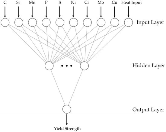
Figure 1.
ANN structure as a diagram.
3. Results
3.1. Multiple Regression Analysis Results
A MRA was conducted using five input parameters: C, Cr, Mo, Cu, and heat input (HI), as identified in previous studies [28,29]. The regression results are expressed in Equation (1).
where the chemical composition is given in wt%, and the heat input is in kJ/cm. The adjusted coefficient of determination (R2) for Equation (1) is 0.9226.
Yield Strength (MPa) = 314 + 352C + 2.96Cr + 24.97Mo + 472Cu − 3.37Heat Input (HI)
3.2. Machine Learning Models
Figure 2 illustrates the R2 values of the prediction models developed using linear regression, decision trees, SVM, and GPR. Models such as the interaction linear regression, coarse decision tree, and cubic SVM models are not presented in Figure 2 because their R2 values are less than 0.50. Among the models considered, six demonstrated R2 values exceeding 0.92: linear regression, robust linear regression, linear SVM, squared exponential GPR, Matern 5/2 GPR, and rational quadratic GPR.
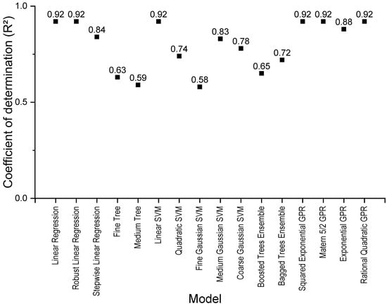
Figure 2.
Prediction models using regression learner application.
For a more comprehensive evaluation of model accuracy, Table 3 summarizes the mean absolute percentage errors (MAPEs) and R2 values for models with an R2 value of 0.90 or higher.
Table 3.
Accuracy of machine learning models.
According to Table 3, the GPR models share an R2 value of 0.92 with linear regression, robust linear regression, and linear SVM but exhibit the lowest MAPEs, i.e., 2.37%, indicating their excellence among the ML models examined. Additionally, the GPR models displayed identical MAPEs of 2.37%, with the predicted yield strength values differing only by decimal places. Among these, the Matern 5/2 GPR can be considered a representative model based on previous research findings [29]. The robust linear regression and linear SVM showed comparable MAPEs of 2.51%, differing insignificantly from the GPR models by only 0.14%. Moreover, the linear regression model deviated by only 0.02% compared to the robust linear regression and linear SVM.
Consequently, among the ML models listed in Table 3, those excluding the squared exponential GPR and rational quadratic GPR, which share nearly identical prediction characteristics with Matern 5/2 GPR, were selected for comparison with the MRA and ANN models.
3.3. Artificial Neural Network (ANN) Models
Figure 3 illustrates the R2 values for the training, validation, and all datasets as the number of nodes in the hidden layer varied from 2 to 20. As shown in Figure 3, when the number of nodes in the hidden layer exceeded 10, the R2 value of the training model remained high, exceeding 0.94. However, the R2 values of the validation models consistently fell below 0.80, notably lower than when the number of nodes in the hidden layer was 10 or fewer.
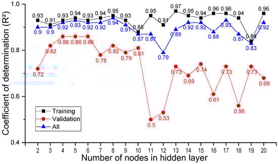
Figure 3.
R2 values for ANN prediction models.
Consequently, in the range of 2–10 nodes in the hidden layer, the disparity between the R2 values of the training and validation models was relatively small. The best performance is observed when the number of nodes is five; the R2 values for the training and validation models are 0.94 and 0.86, respectively. To denote each model by considering a varying number of nodes in the hidden layer, the ANN model can be represented as follows: [number of nodes in the input layer = 10] × [number of nodes in the hidden layer = 2–20] × [number of nodes in the output layer = 1]. Therefore, when the number of nodes in the hidden layer is five, this can be succinctly expressed as 10 × 5 × 1.
Among the training models developed using the 160 datasets, Figure 4 presents a comparison of the MAPEs and R2 values of the MRA, ML, and ANN (10 × 5 × 1). The ANN model exhibited the highest R2 value (0.94) and the lowest MAPE (2.29%), confirming its accuracy as the best prediction model compared to other models.
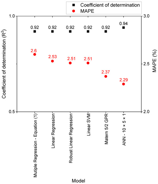
Figure 4.
R2 and MAPE of the prediction models for the training dataset.
A residual analysis was conducted for the models depicted in Figure 4 to evaluate the tendency of the model residuals. Figure 5 illustrates the residuals from the prediction models, revealing a random distribution without any discernible trends in the measured yield strength. The yield strength was determined through tensile testing, using round bar specimens (Figure 6), conducted in accordance with ASTM E8-16: Standard Test Methods for Tension Testing of Metallic Materials [47].
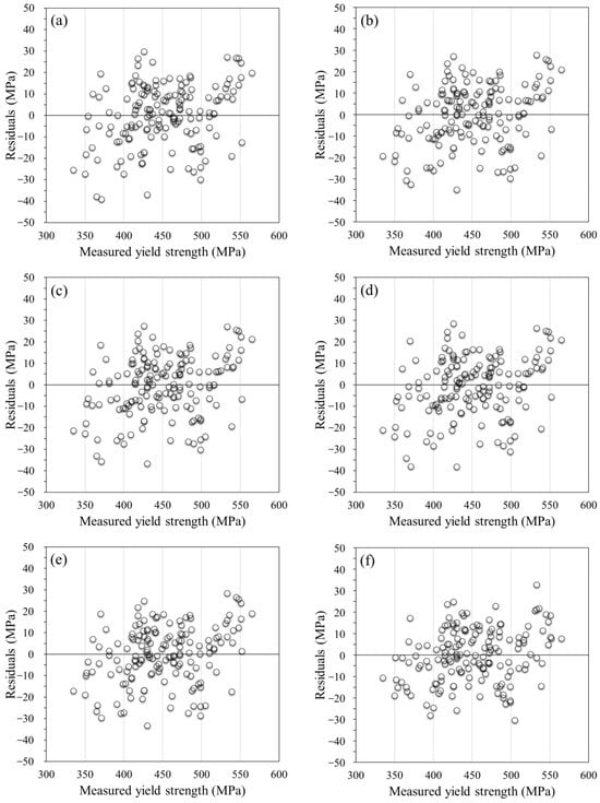
Figure 5.
Residuals plots for regression models: (a) multiple regression—Equation (1); (b) linear regression; (c) robust linear regression; (d) linear SVM; (e) Matern 5/2 GPR; and (f) ANN—10 × 5 × 1 models.
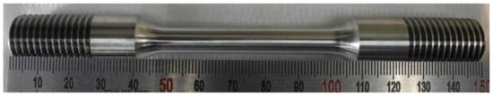
Figure 6.
Type of round tensile test specimen.
3.4. Model Verification Results Using Additional Data Points
The MRA, ML, and ANN models developed in this study were validated using additional data points not utilized during the training step. Table 4 summarizes the MAPE and R2 values to ensure the accuracy of the models during the validation process. The verification results of the previously developed prediction models further confirmed that the ANN model with a 10 × 5 × 1 structure exhibited the lowest MAPE of 3.06% and the highest R2 value of 0.8644 compared to other models. While the Matern 5/2 GPR model exhibited the lowest MAPE among the ML models during the model training step, it recorded the highest MAPE, i.e., 4.78%, and the lowest R2 value, i.e., 0.6097, during the model-verification step. Interestingly, the multiple regression model, which had a higher mean absolute MAPE than the ML models during model training, demonstrated a higher prediction accuracy during model validation. Figure 7 compares the measured yield strength of the additional dataset with that predicted by the developed models.
Table 4.
Accuracy of models for model validation.
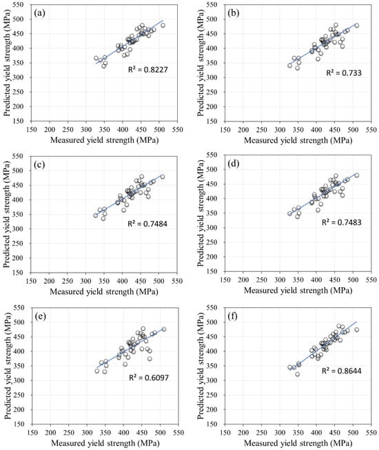
Figure 7.
Correlation between predicted and measured yield strength: (a) multiple regression—Equation (1); (b) linear regression; (c) robust linear regression; (d) linear SVM; (e) Matern 5/2 GPR; and (f) ANN—10 × 5 × 1 models.
Analyzing the correlation between the measured and predicted yield strengths based on Figure 7, we see that the Matern 5/2 GPR model exhibits the lowest R2 value, indicating relatively large discrepancies between the measured and predicted values at certain data points, reaching up to 95 MPa. The coefficient of determination and MAPE of machine learning-based prediction models may be influenced by the attributes of the model and the quantity of data points. The ANN model displayed a maximum difference of 35 MPa between the measured yield strength and the predicted value, the lowest among the compared models. Moreover, the ANN model has relatively fewer data points that deviate significantly from the trend line of the graph compared to the other models, thus ensuring the highest accuracy.
These results confirm that the ANN models overcame the predictive performance limitations observed in the models developed through MRA and ML.
4. Application
4.1. Development of Deep Learning-Based Prediction Model
The ANN model developed in this study was a shallow neural network with one hidden layer. Attempts have been made to develop better prediction models through deep learning-based models using deep neural networks with two or more hidden layers to improve predictive performance. In shallow neural networks, when the number of nodes in the hidden layer exceeded 10, the R2 values of the validation models were consistently below 0.80. Consequently, when developing a deep-learning model with two hidden layers, the number of nodes in each hidden layer ranged from 2 to 10.
Figure 8 illustrates the R2 values for the training, validation, and all datasets of the deep learning-based prediction models with two hidden layers. Similar to the method used to denote shallow neural network models, a deep neural network model with two hidden layers is expressed as [number of nodes in the input layer = 10] × [number of nodes in the first hidden layer = 2–10] × [number of nodes in the second hidden layer = 2–10] × [number of nodes in the output layer = 1]. Figure 8 confirms that the deep-learning models with the highest R2 values for the training models were 10 × 3 × 3 × 1 and 10 × 5 × 5 × 1, with three or five nodes in the hidden layers. Considering the validation results, the R2 value of the 10 × 5 × 5 × 1 model was higher than that of the 10 × 3 × 3 × 1 model, indicating that the 10 × 5 × 5 × 1 model was the best among the deep-learning models with two hidden layers.
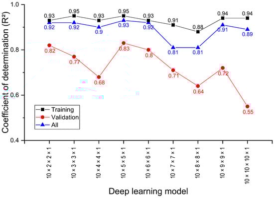
Figure 8.
R2 values for deep-learning prediction models.
Both the shallow neural network with one hidden layer and the deep neural network with two hidden layers achieved high prediction accuracy when the number of nodes was set to five. Consequently, the number of nodes in the hidden layers was fixed at five, and the R2 values were obtained by increasing the number of hidden layers from one to five, as shown in Figure 9.
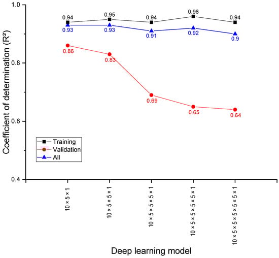
Figure 9.
R2 values of deep-learning models with five nodes in hidden layers.
When the number of hidden layers was set to 1, the R2 value of the training model was 0.94. When the number of hidden layers increased to five, the R2 value remained constant at 0.94. However, with four hidden layers, the R2 value reached its peak at 0.96. Conversely, during model validation, the 10 × 5 × 1 model with one hidden layer exhibited the highest R2 value, i.e., 0.86. As the number of hidden layers increases, the R2 value progressively decreases.
Therefore, despite simultaneously considering changes in the number of nodes and adding two or more hidden layers, the prediction accuracy of the validation model tends to decrease because of overfitting during the training process [48,49]. In this study, the yield strength prediction model for weld metals based on austenitic stainless steel confirmed that the artificial neural network model with a shallow neural network structure of 10 × 5 × 1 was the best.
4.2. Dilution and Yield Strength of Stainless Steel-Based Weld Metal in 3.5–9% Ni Steels
For a specific combination of welding consumables and base metals, the degree of chemical heterogeneity within the weld is influenced by the dilution, which significantly affects the metallurgical microstructure and mechanical properties of steel welds [50,51,52,53,54].
Considering the chemical composition of the final weld metal resulting from the amalgamation of the base metal and welding consumable, the dilution rate can be expressed by the following equation [28,55]:
where D represents the dilution rate; and Cw, Cwc, and Cb denote the elemental compositions of the weld metal, welding consumables, and base metal, respectively.
The ANN-based yield strength prediction model of the weld metal developed in this study can predict the variation in the yield strength of the weld metal, considering dilution when welding 3.5–9% Ni steel, primarily used for low-temperature environments [56,57,58,59,60], using stainless steel-based welding consumables.
To predict the change in the yield strength, four types of base materials (3.5% Ni, 5% Ni, 9% Ni steel, and high-Mn steel) and one fully austenitic stainless steel-based welding consumable were employed, as outlined in Table 5. High-Mn steel was included for comparison with the predicted results for 3.5–9% Ni steel.
Table 5.
Chemical composition of base metals and welding consumables (wt%).
The predicted yield strength with respect to the change in chemical composition owing to dilution is shown in Figure 10. Considering that dilution varies depending on the welding position, current, speed, and heat input, the heat input per unit length was fixed at 10 kJ/cm.
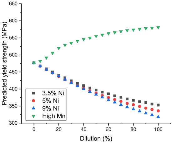
Figure 10.
Predicted yield strength according to dilution and chemical composition changes by base metals.
As shown in Figure 10, a similar trend was observed for the 3.5%, 5%, and 9% Ni steels, where the predicted yield strength decreased as the dilution increased. However, the opposite trend was noted for high-Mn steel, where the predicted yield strength increased as the dilution increased. The main reason for these results is that, in the case of 3.5–9% Ni steel, the C, Cr, and Mo contents in the fully austenitic welding consumable are relatively high compared to the base metals used in this study. Conversely, in the case of high-Mn steel, the primary reason is that the C and Cu contents of the base metal are higher than those of the filler consumables.
Based on the minimum yield strength requirement of 9% Ni steel, 400 MPa [19], the predicted yield strengths are summarized in Table 6 to analyze the limiting dilution at a fixed heat input of 10 kJ/cm for 9% Ni steel, 3.5% Ni, and 5% Ni. According to Table 6, the predicted yield strength was not expected to satisfy 400 MPa for 3.5% Ni steel in the 45–50% dilution range and 5% Ni steel and 9% Ni steel in the 40–45% dilution range.
Table 6.
Results of predicting yield strength according to the increase in dilution for 3.5–9% Ni steels.
While managing with a dilution of 40% or less may be feasible, given the relatively low fixed heat input of 10 kJ/cm, the expected yield strength with increasing heat input for 9% Ni steel is summarized in Table 7. Among the 3.5–9% Ni steels, the 9% Ni steel, predominantly utilized in LNG storage tanks and fuel tanks for LNG-powered ships [19,20,61], was selected. As the heat input increased, the critical dilution required to satisfy the minimum yield strength of 400 MPa decreased. Notably, when the heat input reaches 30 kJ/cm and the dilution is 5%, the predicted yield strength is 399 MPa, which falls short of the minimum requirement of 400 MPa. Hence, to accommodate higher maximum heat input levels while considering dilution, reassessing the composition adjustment of the fully austenitic stainless steel-based welding consumables employed in this study is imperative.
Table 7.
Yield strength prediction according to increase in heat input and dilution for 9% Ni steel.
4.3. Selection of Stainless Steel-Based Welding Consumable to Expand the Range of Heat Input and Dilution Applicable to 9% Ni Steel
To prevent the decrease in yield strength caused by dilution when using an austenitic stainless steel-based welding consumable on 9% Ni steel, the C and Cu contents in the original fully austenitic welding consumable were increased, and the predicted yield strengths are shown in Table 8. The C and Cu contents were incrementally increased by 0.1 wt% and 0.05 wt%, respectively, until the C and Cu contents reached 0.45 wt% and 0.3 wt%, respectively, as listed as the maximum contents in Table 1. To check whether the original fully austenitic microstructure was maintained through chemical composition adjustment and dilution, the Cr and Ni equivalents of the welding consumables in Table 8 are summarized in a Schaeffler diagram, as shown in Figure 11. The original fully austenitic welding consumable resulted in a fully austenitic weld metal microstructure with a dilution of approximately 50%. The modified welding consumables have an increased Ni equivalent owing to the increase in the C content; therefore, the modified welding consumables are advantageous for maintaining a fully austenitic microstructure in the weld metal. In particular, in modified Case 3, the fully austenitic microstructure was maintained up to a dilution of approximately 60%.
Table 8.
Chemical composition of base metal and modified welding consumables (wt%).
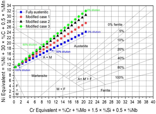
Figure 11.
Cr and Ni equivalents according to chemical composition variation-induced dilution in Schaeffler diagram for austenitic stainless steel-based welding consumables.
Considering that modified welding consumable Case 3 maintained a fully austenitic microstructure up to a dilution of 60%, the previously developed ANN model was used for each welding consumable at heat inputs of 30, 40, and 50 kJ/cm up to a dilution of 60% (the original fully austenitic welding consumable had a predicted yield strength of only 407 MPa, even without any dilution, at a heat input of 30 kJ/cm; therefore, only those data were included). The yield strengths predicted by the model are listed in Table 9. By increasing the C and Cu contents, the dilution and heat input ranges that can secure a yield strength of at least 400 MPa can be expanded. In particular, the modified welding consumables (Case 3) could predict a yield strength of 409 MPa, which satisfies a minimum of 400 MPa at a heat input of 50 kJ/cm and a dilution of 40%. Therefore, various applications are feasible with the ANN model, which has a better prediction performance than conventional MRA and ML.
Table 9.
Yield strength prediction results according to increased heat input and dilution of modified welding consumables for 9% Ni steel.
5. Conclusions
In this study, an artificial neural network (ANN)-based model was developed to predict the yield strength of a weld metal using austenitic stainless steel-based welding materials. The following conclusions were drawn:
- Among the training models developed using multiple regression analysis (MRA), machine learning (ML), and an ANN with 160 datasets, the ANN (10 × 5 × 1) model with five nodes in one hidden layer emerged as the best prediction model, exhibiting the highest R2 value (0.94) and the lowest MAPE (2.29%).
- In the model verification, the ANN (10 × 5 × 1) model also demonstrated a superior prediction performance compared with the MRA and ML models, achieving the highest R2 value, i.e., 0.8644, and the lowest MAPE, i.e., 3.06%. These results confirm that ANN models minimize overfitting and enhance prediction performance compared to the MRA and ML models.
- Despite simultaneously considering changes in the number of nodes and adding two or more hidden layers, the prediction accuracy of the validation model tends to decrease because of overfitting during the training process. The yield strength prediction model for weld metals based on austenitic stainless steel confirmed that the artificial neural network model with a shallow neural network structure of 10 × 5 × 1 was the most effective.
The ANN model developed in this study can effectively forecast variations in the yield strength and microstructure resulting from the thermal history and dilution during the welding of 3.5–9% Ni steels with stainless steel-based welding consumables. The prediction model optimized the chemical composition of austenitic stainless steel-based welding consumables in welding 9% Ni steel.
Hence, this study lays the groundwork for the development of a prediction model leveraging not only machine learning (ML) but also the multiple regression analysis (MRA) for predicting the yield strength of stainless-steel welds using artificial intelligence, such as artificial neural networks (ANNs). Unlike MRA, which struggles with non-linear problems as the dataset grows, ANN excels in solving such complexities, thus enabling the creation of more accurate prediction models. With the acquisition of reliable and comprehensive data across various materials, this approach holds promise for predicting the physical properties of diverse welds.
Author Contributions
Conceptualization, S.P. and C.K.; data preparation, S.P.; software, S.P. investigation, S.P.; resources, C.K. and N.K.; writing—original draft preparation, S.P.; writing—review and editing, C.K.; supervision, N.K.; project administration, C.K.; funding acquisition, N.K. All authors have read and agreed to the published version of the manuscript.
Funding
This work was supported by the Technology Innovation Program (Grant No. 20022454 and 20010778), funded by the Ministry of Trade, Industry, and Energy (MOTIE, Korea).
Data Availability Statement
The data presented in this study are available on request from the corresponding author. The data are not publicly available due to privacy.
Conflicts of Interest
The authors declare no conflicts of interest.
References
- Ohkubo, N.; Miyakusu, K.; Uematsu, Y.K. Hiroshi Effect of alloying elements on the mechanical properties of the stable austenitic stainless steel. ISIJ Int. 1994, 34, 764–772. [Google Scholar] [CrossRef]
- Sieurin, H.; Zander, J.; Sandström, R. Modelling solid solution hardening in stainless steels. Mater. Sci. Eng. A 2006, 415, 66–71. [Google Scholar] [CrossRef]
- Booker, M.K.; Sikka, V.K. Effects of Composition Variables on the Tensile Properties of Type 304 Stainless Steel; Oak Ridge National Lab: Oak Ridge, TN, USA, 1977. [Google Scholar]
- Xie, Q.; Suvarna, M.; Li, J.; Zhu, X.; Cai, J.; Wang, X. Online prediction of mechanical properties of hot rolled steel plate using machine learning. Mater. Des. 2021, 197, 109201. [Google Scholar] [CrossRef]
- Narayana, P.L.; Lee, S.W.; Park, C.H.; Yeom, J.-T.; Hong, J.-K.; Maurya, A.K.; Reddy, N.S. Modeling high-temperature mechanical properties of austenitic stainless steels by neural networks. Comput. Mater. Sci. 2020, 179, 109617. [Google Scholar] [CrossRef]
- Stoll, A.; Benner, P. Machine learning for material characterization with an application for predicting mechanical properties. GAMM-Mitteilungen 2021, 44, e202100003. [Google Scholar] [CrossRef]
- Guo, S.; Yu, J.; Liu, X.; Wang, C.; Jiang, Q. A predicting model for properties of steel using the industrial big data based on machine learning. Comput. Mater. Sci. 2019, 160, 95–104. [Google Scholar] [CrossRef]
- Lee, J.I.; Um, K.W. A comparison in a back-bead prediction of gas metal arc welding using multiple regression analysis and artificial neural network. J. Opt. Lasers Eng. 2000, 34, 149–158. [Google Scholar] [CrossRef]
- Acherjee, B.; Mondal, S.; Tudu, B.; Misra, D. Application of artificial neural network for predicting weld quality in laser transmission welding of thermoplastics. Appl. Soft. Comput. 2011, 11, 2548–2555. [Google Scholar] [CrossRef]
- Jones, D.M.; Watton, J.; Brown, K.J. Comparison of hot rolled steel mechanical property prediction models using linear multiple regression, non-linear multiple regression and non-linear artificial neural networks. Ironmak. Steelmak. 2005, 32, 435–442. [Google Scholar] [CrossRef]
- Sarkar, A.; Dey, P.; Rai, R.N.; Saha, S.C. A comparative study of multiple regression analysis and back propagation neural network approaches on plain carbon steel in submerged-arc welding. Sādhanā 2016, 41, 549–559. [Google Scholar] [CrossRef]
- Wang, Y.-M.; Elhag, T.M.S. A comparison of neural network, evidential reasoning and multiple regression analysis in modelling bridge risks. Expert. Syst. Appl. 2007, 32, 336–348. [Google Scholar] [CrossRef]
- Nguyen, N.; Cripps, A. Predicting Housing Value: A Comparison of Multiple Regression Analysis and Artificial Neural Networks. J. Real. Estate Res. 2001, 22, 313–336. [Google Scholar] [CrossRef]
- Kim, J.-H.; Kim, B.K.; Kim, D.-I.; Choi, P.-P.; Raabe, D.; Yi, K.-W. The role of grain boundaries in the initial oxidation behavior of austenitic stainless steel containing alloyed Cu at 700 °C for advanced thermal power plant applications. Corros. Sci. 2015, 96, 52–66. [Google Scholar] [CrossRef]
- Switzner, N.; Yu, Z. Austenitic Stainless Steel Cladding Interface Microstructures Evaluated for Petrochemical Applications. Weld. J. 2019, 98, 50–61. [Google Scholar] [CrossRef]
- Park, W.S.; Yoo, S.W.; Kim, M.H.; Lee, J.M. Strain-rate effects on the mechanical behavior of the AISI 300 series of austenitic stainless steel under cryogenic environments. Mater. Des. 2010, 31, 3630–3640. [Google Scholar] [CrossRef]
- Baek, J.H.; Kim, Y.P.; Kim, W.S.; Kho, Y.T. Effect of Temperature on the Charpy Impact and CTOD Values of Type 304 Stainless Steel Pipeline for LNG Transmission. KSME Int. J. 2002, 16, 1064–1071. [Google Scholar] [CrossRef]
- Kim, J.-H.; Choi, S.-W.; Park, D.-H.; Lee, J.-M. Charpy impact properties of stainless steel weldment in liquefied natural gas pipelines: Effect of low temperatures. Mater. Des. 2015, 65, 914–922. [Google Scholar] [CrossRef]
- Park, T.U.; Jeong, Y.C.; Im, H.D.; Choi, C.H.; Kil, W. Development and Evaluation of Stainless Steel-Base Flux-Cored Wires for 9% Nickel Steel. JWJ 2022, 40, 367–376. [Google Scholar] [CrossRef]
- Kim, B.E.; Park, J.Y.; Lee, J.S.; Lee, J.I.; Kim, M.H. Effects of the welding process and consumables on the fracture behavior of 9 wt.% nickel steel. Exp. Tech. 2019, 44, 175–186. [Google Scholar] [CrossRef]
- Choi, M.; Lee, J.; Nam, H.; Kang, N.; Kim, M.; Cho, D. Tensile and Microstructural Characteristics of Fe-24Mn Steel Welds for Cryogenic Applications. Met. Mater. Int. 2020, 26, 240–247. [Google Scholar] [CrossRef]
- Park, T.U.; Jung, D.H.; Park, J.H.; Kim, J.H.; Han, I.W. Changes in the mechanical properties and microstructure of high manganese steel by high heat input welding and general welding processes. JWJ 2022, 40, 33–39. [Google Scholar] [CrossRef]
- Park, G.; Jeong, S.; Lee, C. Fusion weldabilities of advanced high manganese steels: A review. Met. Mater. Int. 2020, 27, 2046–2058. [Google Scholar] [CrossRef]
- Yoo, J.; Kim, B.; Park, Y.; Lee, C. Microstructural evolution and solidification cracking susceptibility of Fe-18Mn-0.6C-xAl steel welds. J. Mater. Sci. 2015, 50, 279–286. [Google Scholar] [CrossRef]
- Avery, R.E.; Parsons, D. Welding stainless and 9% nickel steel cryogenic vessels. Weld. J. 1995, 74, 45–50. [Google Scholar]
- Banovic, S.W.; Dupont, J.N.; Marder, A.R. Dilution and microsegregation in dissimilar metal welds between super austenitic stainless steel and nickel base alloys. Sci. Technol. Weld. Join. 2013, 7, 374–383. [Google Scholar] [CrossRef]
- Dupont, J.N.; Banovic, S.W.; Marder, A.R. Microstructural Evolution and Weldability of Dissimilar Welds between a Super Austenitic Stainless Steel and Nickel-Based Alloys. Weld. J. 2003, 82, 125. [Google Scholar]
- Park, S.; Won, J.; Yoo, S.; Moon, B.; Kim, C.; Kang, N. Influence of welding position and dilution on mechanical properties and strengthening design of flux cored arc weld metal for high manganese steels. Int. J. Adv. Manuf. Technol. 2024, 130, 3509–3523. [Google Scholar] [CrossRef]
- Park, S.; Choi, M.; Kim, D.; Kim, C.; Kang, N. Modeling Yield Strength of Austenitic Stainless Steel Welds Using Multiple Regression Analysis and Machine Learning. Metals 2023, 13, 1625. [Google Scholar] [CrossRef]
- Kusiak, J.; Kuziak, R. Modelling of microstructure and mechanical properties of steel using the artificial neural network. J. Mater. Proc. Technol. 2002, 127, 115–121. [Google Scholar] [CrossRef]
- Bahrami, A.; Mousavi Anijdan, S.H.; Ekrami, A. Prediction of mechanical properties of DP steels using neural network model. J. Alloy Compd. 2005, 392, 177–182. [Google Scholar] [CrossRef]
- Sterjovski, Z.; Nolan, D.; Carpenter, K.R.; Dunne, D.P.; Norrish, J. Artificial neural networks for modelling the mechanical properties of steels in various applications. J. Mater. Proc. Technol. 2005, 170, 536–544. [Google Scholar] [CrossRef]
- Ghaisari, J.; Jannesari, H.; Vatani, M. Artificial neural network predictors for mechanical properties of cold rolling products. Adv. Eng. Softw. 2012, 45, 91–99. [Google Scholar] [CrossRef]
- Merayo, D.; Rodriguez-Prieto, A.; Camacho, A.M. Prediction of Mechanical Properties by Artificial Neural Networks to Characterize the Plastic Behavior of Aluminum Alloys. Materials 2020, 13, 5227. [Google Scholar] [CrossRef] [PubMed]
- Merayo, D.; Rodriguez-Prieto, A.; Camacho, A.M. Prediction of Physical and Mechanical Properties for Metallic Materials Selection Using Big Data and Artificial Neural Networks. IEEE Access 2020, 8, 13444–13456. [Google Scholar] [CrossRef]
- Wang, Y.; Wu, X.; Li, X.; Xie, Z.; Liu, R.; Liu, W.; Zhang, Y.; Xu, Y.; Liu, C. Prediction and Analysis of Tensile Properties of Austenitic Stainless Steel Using Artificial Neural Network. Metals 2020, 10, 234. [Google Scholar] [CrossRef]
- Wei, Y.; Bhadeshia, H.K.D.H.; Sourmail, T. Mechanical property prediction of commercially pure titanium welds with artificial neural network. J. Mater. Sci. Technol. 2005, 21, 403–407. [Google Scholar]
- Okuyucu, H.; Kurt, A.; Arcaklioglu, E. Artificial neural network application to the friction stir welding of aluminum plates. Mater. Des. 2007, 28, 78–84. [Google Scholar] [CrossRef]
- Maleki, E. Artificial neural networks application for modeling of friction stir welding effects on mechanical properties of 7075-T6 aluminum alloy. IOP Conf. Ser. Mater. Sci. Eng. 2015, 103, 012034. [Google Scholar] [CrossRef]
- Kim, T.-W.; Ju, W.-H.; Jeon, S.-H.; Kim, Y.-C. A Study on Mechanical Properties of Austenitic Stainless Steel Welds Using ArcTig Welding. JWJ 2022, 40, 343–351. [Google Scholar] [CrossRef]
- Cui, Y.; Lundin, C.D.; Hariharan, V. Mechanical behavior of austenitic stainless steel weld metals with microfissures. J. Mater. Proc. Technol. 2006, 171, 150–155. [Google Scholar] [CrossRef]
- Piatti, G.; Vedani, M. Relation between tensile properties and microstructure in type 316 stainless steel SA weld metal. J. Mater. Sci. 1990, 25, 4285–4297. [Google Scholar] [CrossRef]
- Ward, A.L.; Blackburn, L.D. Elevated Temperature Tensile Properties of Weld-Deposited Austenitic Stainless Steels. J. Eng. Mater. Technol. 1976, 98, 213–220. [Google Scholar] [CrossRef]
- Moteshakker, A.; Danaee, I.; Moeinifar, S.; Ashrafi, A. Hardness and tensile properties of dissimilar welds joints between SAF 2205 and AISI 316L. Sci. Technol. Weld Join 2016, 21, 1–10. [Google Scholar] [CrossRef]
- Lee, K.; Kang, S.; Kang, M.; Yi, S.; Hyun, S.; Kim, C. Modeling of Laser Welds Using Machine Learning Algorithm Part I: Penetration Depth for Laser Overlap Al/Cu Dissimilar Metal Welds. JWJ 2021, 39, 27–35. [Google Scholar] [CrossRef]
- You, H.; Kang, M.; Yi, S.; Hyun, S.; Kim, C. Modeling of Laser Welds Using Machine Learning Algorithm Part II: Geometry and Mechanical Behaviors of Laser Overlap Welded High Strength Steel Sheets. JWJ 2021, 39, 36–44. [Google Scholar] [CrossRef]
- ASTM E8; Standard Test Methods for Tension Testing of Metallic Materials. ASTM: West Conshohocken, PA, USA, 2016.
- Uzair, M.; Jamil, N. Effects of Hidden Layers on the Efficiency of Neural networks. In Proceedings of the 2020 IEEE 23rd International Multitopic Conference, INMIC, Bahawalpur, Pakistan, 5–7 November 2020. [Google Scholar]
- Bejani, M.M.; Ghatee, M. A systematic review on overfitting control in shallow and deep neural networks. Artif. Intell. Rev. 2021, 54, 6391–6438. [Google Scholar] [CrossRef]
- Hunt, A.C.; Kluken, A.O.; Edwards, G.R. Heat Input and Dilution Effects in Microalloyed Steel Weld Metals. Weld. J. 1994, 73, 9s–15s. [Google Scholar]
- Ramjaun, T.I.; Stone, H.J.; Karlsson, L.; Kelleher, J.; Ooi, S.W.; Dalaei, K.; Rebelo Kornmeier, J.; Bhadeshia, H.K.D.H. Effects of dilution and baseplate strength on stress distributions in multipass welds deposited using low transformation temperature filler alloys. Sci. Technol. Weld. Join. 2014, 19, 461–467. [Google Scholar] [CrossRef]
- Halbauer, L.; Buchwalder, A.; Zenker, R.; Biermann, H. The influence of dilution on dissimilar weld joints with high-alloy TRIP/TWIP steels. Weld. World 2016, 60, 645–652. [Google Scholar] [CrossRef]
- Sun, Y.L.; Obasi, G.; Hamelin, C.J.; Vasileiou, A.N.; Flint, T.F.; Balakrishnan, J.; Smith, M.C.; Francis, J.A. Effects of dilution on alloy content and microstructure in multi-pass steel welds. J. Mater. Proc. Technol. 2019, 265, 71–86. [Google Scholar] [CrossRef]
- Sun, Y.L.; Hamelin, C.J.; Flint, T.F.; Vasileiou, A.N.; Francis, J.A.; Smith, M.C. Prediction of Dilution and Its Impact on the Metallurgical and Mechanical Behavior of a Multipass Steel Weldment. J. Press. Vessel. Technol. 2019, 141, 061405. [Google Scholar] [CrossRef]
- Banovic, S.W.; DuPont, I.N.; Marder, A.R. Dilution control in gas-tungsten-arc welds involving superaustenitic stainless steels and nickel-based alloys. Metall. Mater. Trans. B 2001, 32, 1171–1176. [Google Scholar] [CrossRef]
- Ishimaru, Y.; Kobayashi, H.; Okada, T.; Tomiyasu, F. Automatic Welding of 3.5% Nickel Steel. Weld. J. 1978, 57, 273s–280s. [Google Scholar]
- McHenry, H.I.; Reed, R.P. Fracture Behavior of the HeatAffected Zone in 5% Ni Steel Weldments. Weld. Res. Suppl. 1977, 4, 104–112. [Google Scholar]
- Sarno, D.A.; Bruner, J.P.; Kampschaefer, G.E. Fracture Toughness of 5% Nickel Steel Weldments. Weld. J. 1974, 53, 486–494. [Google Scholar]
- Xin, D.; Cai, Y.; Hua, X. Effect of preheating on microstructure and low-temperature toughness for coarse-grained heat-affected zone of 5% Ni steel joint made by laser welding. Weld. World 2019, 63, 1229–1241. [Google Scholar] [CrossRef]
- Kern, A.; Schriever, U.; Stumpfe, J. Development of 9% Nickel Steel for LNG Applications. Steel Res. Int. 2007, 78, 189–194. [Google Scholar] [CrossRef]
- Kim, T.Y.; Yoon, S.W.; Kim, J.H.; Kim, M.H. Fatigue and fracture behavior of cryogenic materials applied to LNG fuel storage tanks for coastal ships. Metals 2021, 11, 1899. [Google Scholar] [CrossRef]
Disclaimer/Publisher’s Note: The statements, opinions and data contained in all publications are solely those of the individual author(s) and contributor(s) and not of MDPI and/or the editor(s). MDPI and/or the editor(s) disclaim responsibility for any injury to people or property resulting from any ideas, methods, instructions or products referred to in the content. |
© 2024 by the authors. Licensee MDPI, Basel, Switzerland. This article is an open access article distributed under the terms and conditions of the Creative Commons Attribution (CC BY) license (https://creativecommons.org/licenses/by/4.0/).