A Scalogram-Based CNN Approach for Audio Classification in Construction Sites

Abstract

The automatic monitoring of activities in construction sites through the proper use of acoustic signals is a recent field of research that is currently in continuous evolution. In particular, the use of techniques based on Convolutional Neural Networks (CNNs) working on the spectrogram of the signal or its mel-scale variants was demonstrated to be quite successful. Nevertheless, the spectrogram has some limitations, which are due to the intrinsic trade-off between temporal and spectral resolutions. In order to overcome these limitations, in this paper, we propose employing the scalogramas a proper time–frequency representation of the audio signal. The scalogram is defined as the square modulus of the Continuous Wavelet Transform (CWT) and is known as a powerful tool for analyzing real-world signals. Experimental results, obtained on real-world sounds recorded in construction sites, have demonstrated the effectiveness of the proposed approach, which is able to clearly outperform most state-of-the-art solutions.

1. Introduction

In recent years significant research efforts have been made in the field of Environmental Sound Classification (ESC) [1], allowing significant results to be obtained in practical sound classification applications. This initiative has been enabled by the use of Convolutional Neural Networks (CNNs), which allowed a superior performance in image processing problems [2] to be obtained. In order to extend the use of CNNs to the field of audio processing, the audio input signal is usually transformed into suitable bi-dimensional image-like representations, such as spectrograms, mel-scale spectrograms, and other similar methods [3,4].

Recently, the approaches employed in ESC have been transferred to advancing the construction domain by converting vision-based work monitoring and management systems into audio-based ones [5,6,7]. In fact, audio-based systems not only are more cost-effective than video-based ones, but they also work more effectively in a construction field when sources are far from the light of sight of sensors, making these systems very flexible and appropriate for combining other sensor-based applications or Artificial Intelligence (AI)-based technologies [7]. Furthermore, the amount of memory and data flow needed to handle audio data is much smaller than the one needed for video data. In addition, audio-based systems outperform accelerometer-based ones since there is no need to place sensors onboard, thus promoting 360-degree-based activity detection and surveillance without having an illumination issue [8].

Such audio-based systems can be successfully used as Automatic Construction Site Monitoring (ACSM) tools [7,9,10,11], which can represent an invaluable instrument for project managers to promptly identify severe and urgent problems in fieldwork and quickly react to unexpected safety and hazard issues [12,13,14,15,16].

ACSM systems are usually implemented by exploiting both machine learning (ML) and deep learning (DL) techniques [17]. Specifically, several ML approaches, including Support Vector Machines (SVMs), the k-Nearest Neighbors (k-NN) algorithm, the Multilayer Perceptron (MLP), random forests, Echo State Networks (ESN), and others, have already demonstrated their effectiveness in properly performing activity identification and detection in a construction site [5,16]. However, DL approaches generally outperform ML-based solutions providing much improved results [6]. We expect that DL techniques including CNNs, Deep Recurrent Neural Networks (DRNNs) implemented with the Long Short-Term Memory (LSTM) cell, Deep Belief Networks (DBNs), Deep ESNs, and others can produce more suitable and qualified performances than ML ones for robustly managing construction work and safety issues.

Approaches based on CNNs have demonstrated good flexibility and considerably convincing performance in these applications. In fact, CNNs exhibit advanced accuracy in image classification [18]. In order to meet the bi-dimensional format of images, the audio waveform can be transformed into a bi-dimensional representation by a proper time–frequency transformation. The main time–frequency representation used in audio applications is the spectrogram, i.e., the squared magnitude of the Short Time Fourier Transform (STFT) [19,20]. The spectrogram is very rich in peculiar information that can be successfully exploited by CNNs. Instead of using the STFT spectrogram, in audio processing, it is very common to use some well-known variants, such as the constant-Q spectrogram, which uses a log-frequency mapping, and the mel-scale spectrogram, which uses the mel-scale of frequency to better capture the intrinsic characteristic of the human ear. Similarly, the Bark and/or ERB scales can be used, producing other variants of the spectrogram [21].

Although the spectrogram representation and its variants provide an effective way to extract features from audio signals, they entail some limitations due to the unavoidable trade-off between the time and frequency resolutions. Unfortunately, it is hard to provide an adequate resolution in both domains: a shorter time window provides a better time resolution, but it reduces the frequency resolution, while using longer time windows improves the frequency resolution but obtains a worse time resolution. Even if some solutions have been proposed to mitigate such an unwanted effect (such as the time–frequency reassignment and synchrosqueezing approach [22]), the problem can still affect the performance of deep learning methods. Moreover, the issue is also complicated by the fact that sound information is usually available at different time scales that cannot be captured by the STFT.

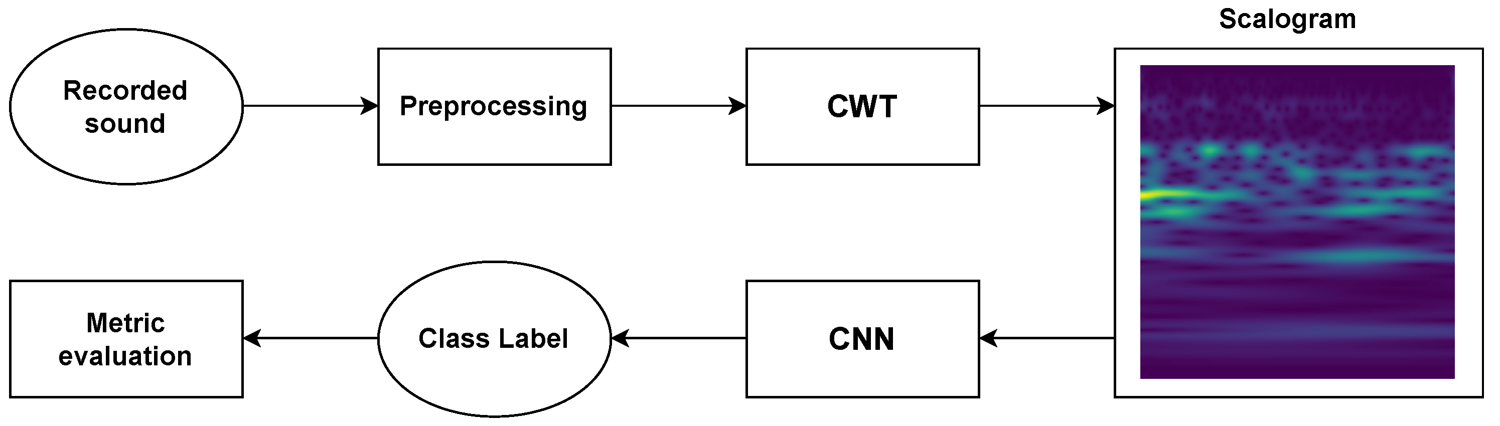
Motivated by these considerations, in this paper, we propose a new approach for the automatic monitoring of construction sites based on CNNs and scalograms. The scalogram was defined as the squared magnitude of the Continuous Wavelet Transform (CWT) [23]. By overcoming the intrinsic time–frequency trade-off, the scalogram is expected to offer an advanced and robust tool to improve the overall accuracy and performance of ACSM systems. In addition, the wavelet transform allows to it work at different time scales, which is a useful characteristic for the processing of audio data. Hence, the main idea of the paper is to use the scalogram instead of the spectrogram as the input to a CNN-based deep learning model. Although the methodology is not new, the proposed idea has been extensively tested on real data acquired in construction sites and, compared to most popular state-of-the-art methodologies, shows clear and significant improvements.

The rest of this paper is organized as follows. Section 2 shows the related work. Section 3 introduces the CWT, while Section 4 describes the proposed approach. Then, Section 5 explains the adopted experimental setup. Section 6 describes some implementation aspects, while Section 7 shows the obtained numerical results and confirms the effectiveness of the proposed idea. Finally, Section 8 concludes the work and outlines some hints for future research.

2. Related Work

In the digital era, great and increasing attention has been devoted to research on automated methods for real-time monitoring of activities in construction sites [15,24,25]. These modern approaches are able to offer better performance with respect to the most traditional techniques, which are typically based on manual collection of on-site work data and human-based construction project monitoring. In fact, these activities are typically time-consuming, inaccurate, costly, and labor-intensive [13]. In the last years, the literature related to applications of deep learning techniques to the construction industry has been continuously increasing [26,27]. In particular, many works have been published describing proper exploitation of audio data [5,16].

The work of Cao et al. in [28] was one of the first attempts in this direction. They introduced an algorithm based on the processing of acoustic data for the classification of four representative excavators. This approach is based on some acoustic statistical features. Namely, for the first time the short frame energy ratio, concentration of spectrum amplitude ratio, truncated energy range, and interval of pulse (i.e., the time interval between two consecutive peaks) were developed in order to characterize acoustic signals. The obtained results were quite effective for this kind of source; however, no other types of equipment were considered.

Paper [29] proposed the construction of a dataset of four classes of equipment and tested several ML classifiers. The results obtained in this work were aligned to those shown in [5], which compared and assessed the accuracy of 17 classifiers on nine classes of equipment. These two papers work on both temporal and spectral features extracted from audio signals. Similarly, Ref. [30] compared some ML approaches on five input classes by using a single in-pocket smartphone, obtaining similar numerical results.

Akbal et al. [14] proposed an SVM classifier. After an iterative neighborhood component analysis selector chooses the most significant features extracted from audio signals, this classifier produces an effective accuracy on two experimental scenarios. Moreover, Kim et al. [7] proposed a sound localization framework for construction site monitoring able to work in both indoor and outdoor scenarios.

Maccagno et al. [31] proposed a deep CNN-based approach for the classification of five pieces of construction site machinery and equipment. This customized CNN is fed by the STFT spectrograms extracted from different-sized audio chunks. Similarly, Sherafat et al. [32] proposed an approach for multiple-equipment activity recognition using CNNs, tested on both synthetic and real-world equipment sound mixtures. Different from [31], this work implements a data augmentation method to enlarge the used dataset. Moreover, this model uses a moving mode function to find the most frequent labels in a period ranging from 0.5 to 2 s, which generates an acceptable output accuracy. The idea to join different output labels inside a short time period was also exploited in [33,34], which implement a Deep Belief Network (DBN) classifier and an Echo State Network (ESN), respectively.

Kim et al. in [35] applied CNNs and RNNs to spectrograms for monitoring concrete pouring work in construction sites, while Xiong et al. in [6] used a convolutional RNN (CRNN) for activity monitoring. Moreover, Peng et al. in [36] used a similar DL approach for a denoising application in construction sites. On the other hand, Akbal et al. [37] proposed an approach, called DesPatNet25, which extracts 25 feature vectors from audio signals by using the data encryption standard cipher and adopts a k-NN and an SVM classifier to identify seven classes.

Additionally, some other approaches also fused information from two different modalities. For example, the work in [38] used an SVM classifier by combining both auditory and kinematics features, showing an improvement of about 5% when compared to the use of only individual sources of data. Similarly, Ref. [39] exploited visual and kinematic features, while [40] utilized location data from a GPS and a vision-based model to detect construction equipment. Finally, a multimodal audio–video approach was presented in [41], based on the use of different correlations of visual and auditory features, which has shown an overall improvement in detection performance.

In addition, Elelu et al. in [42] exploited CNN architectures to automatically detect collision hazards between construction equipment. Similarly, the work in [43] presented a critical review of recent DL approaches for fully embracing construction workers’ awareness of hazardous situations in construction sites by the employment of auditory systems.

Most of the DL approaches described in this section work on the spectrogram extracted from audio signals or some variants, such as the mel-scaled spectrogram. However, the idea of exploiting different time scales (which is an intrinsic property of audio signals) can be used to improve the overall accuracy of such methodologies. For this purpose, the use of scalograms can be recommended. In fact, while spectrograms are suitable for the analysis of stationary signals providing a uniform resolution, the scalogram is able to localize transients in non-stationary signals. Recently, in fact, Ref. [44] introduced a wavelet filter bank for the audio scene modeling task. A deep CNN fed by the scalogram of data outperformed the results provided by the mel spectrogram. However, differently from our approach, the work in [44] considers a scalogram of smaller size and a simpler CNN architecture. The work in [45] adopted scalograms for removing background noise in the fault diagnosis of rotating machinery, obtaining excellent experimental results. However, differently from our approach, given the specific nature of the considered sounds, the authors used a low sampling frequency and frame size, resulting in a very small scalogram size ($64\times 64$ pixels). Interestingly enough, [45] considers three different methods to obtain the scalograms, including the CWT. No significant statistical differences have been observed between such methods. In addition, a couple of papers used scalograms also for audio scene classification purposes [46,47]. Both of these works showed very good results when compared to previous solutions. As a matter of fact, the use of the scalogram results in a general improvement in performance as highlighted in all these works. Specifically, the work in [46] exploits a pre-trained CNN to extract, at a specific architecture-dependent layer, useful features to be used by a subsequent linear SVM classifier for the identification of ten environmental categories. This work also uses AlexNet but, differently from our approach, it does not train the CNN layers and does not adopt fully connected layers as a classifier. The work in [47] again uses a pre-trained AlexNet or VGG16/19 nets to extract meaningful features, but, differently, it exploits a Bidirectional Gated Recurrent Neural Network followed by a highway layer to classify fifteen classes. Differently from our approach, the authors of [47] adopt an early data fusion technique by feeding the proposed model with a three-channel image composed of a spectrogram, a scalogram extracted with the Bump wavelet, and a scalogram obtained with the Morse wavelet. However, the high computational cost of this approach, compared with the proposed one, makes it not very suitable for working with the construction site sounds, where only a small number of classes are present.

3. The Continuous Wavelet Transform (CWT) and the Scalogram

In order to overcome the trade-off between the time and frequency resolution in STFT, the Continuous Wavelet Transform (CWT) was introduced [23]. The CWT acts as a “mathematical” microscope in the sense that different parts of the signal may be examined by adjusting the focus.

Given a stationary signal $x\left(t\right)$, the CWT is defined as the product of $x\left(t\right)$ with the following basis function family:

$${\Psi }_{\tau ,a}\left(t\right)={\left|a\right|}^{-1/2}\Psi \left(\frac{t-\tau }{a}\right),$$

(1)

where $a\ne 0$ is a scaling factor (also known as dilation parameter) and $\tau$ is the time delay, i.e., ${\Psi }_{\tau ,a}\left(t\right)$ is a scaled and translated version of the mother wavelet function $\Psi \left(t\right)$. Hence, the CWT of signal $x\left(t\right)$ is formulated as:

$$W_x(\tau ,a)={\left|a\right|}^{-1/2}{\int }_{-\infty }^{\infty }x\left(t\right){\Psi }^{*}\left(\frac{t-\tau }{a}\right)dt,$$

(2)

where ${}^{*}$ represents the complex conjugation operator. The delay parameter $\tau$ provides the time position of the wavelet ${\Psi }_{\tau ,a}\left(t\right)$, while the scaling factor a rules its frequency content. For $\left|a\right|<<1$, the wavelet ${\Psi }_{\tau ,a}\left(t\right)$ is a very concentrated and narrow version of the mother wavelet $\Psi \left(t\right)$, with a frequency content mainly condensed at high frequencies. On the other hand, for $\left|a\right|>>1$, the wavelet ${\Psi }_{\tau ,a}\left(t\right)$ is much more broadened and concentrated towards low frequencies.

In the wavelet analysis, the similarity between the signal $x\left(t\right)$ and the wavelet ${\Psi }_{\tau ,a}\left(t\right)$ is measured as $\tau$ and a vary. Dilation by a factor $1/a$ results in different enlargements of the signal with distinct resolutions. Specifically, the properties of the time–frequency resolution of the CWT are summarized as follows:

• The temporal resolution $\Delta \tau$ varies inversely to the carrier frequency ${\omega }_0$ of the wavelet ${\Psi }_{\tau ,a}\left(t\right)$; therefore, it can be made arbitrarily small at high frequencies.
• The frequency resolution $\Delta \omega$ varies linearly with the carrier frequency ${\omega }_0$ of the wavelet ${\Psi }_{\tau ,a}\left(t\right)$; therefore, it can be made arbitrarily small at low frequencies.

Hence, the CWT is well suited for the analysis of non-stationary signals containing high-frequency transients superimposed on long-lasting low-frequency components [23].

The CWT implements the signal analysis at various time scales. For this reason, the squared absolute value of the CWT is called a scalogram, and it is defined as:

$$\mathcal{S}(\tau ,a)\triangleq {\left|W_x(\tau ,a)\right|}^2=\frac{1}{a}{\left|{\int }_{-\infty }^{\infty }x\left(t\right){\Psi }^{*}\left(\frac{t-\tau }{a}\right)dt\right|}^2.$$

(3)

The scalogram $\mathcal{S}(\tau ,a)$ provides a bi-dimensional graphical representation of the signal energy at the specific scale parameter a and time location $\tau$.

In general, the mother wavelet $\Psi \left(t\right)$ can be any band-pass function [23]. The Haar wavelet is the simplest example of a wavelet, while the Daubechies one is a more sophisticated example. Both of these wavelets have a finite (and compact) support in time. The Daubechies wavelet has a longer length than the Haar wavelet and is therefore less localized than the latter. However, the Daubechies wavelet is continuous and has a better frequency resolution than the Haar one [23]. Other famous wavelet families are the Mexican Hat wavelet (which is proportional to the second derivative function of the Gaussian probability density function), the Bump wavelet, the generalized Morse wavelet, and the Morlet one, also known as the Gabor wavelet. This last wavelet is composed of a complex exponential multiplied by a Gaussian window, and it is very suitable for audio and vision applications since it is closely related to human perception. For this purpose, we remark that it is strongly related to the short-time analysis performed by the peripheral auditory system and to the mechanical spectral analysis performed by the basilar membrane in the human ear [48]. As a matter of fact, the Morlet wavelet is the most widely used wavelet for audio applications [49], and its effectiveness has been shown in analyzing machine sounds [50]. Motivated by these considerations, in the rest of the paper, we use the Morlet wavelet, which is defined as:

$$\Psi \left(t\right)=C_{\psi }{e}^{-\frac{t^2}{2{\sigma }^2}}{e}^{j{\omega }_{0}t},$$

(4)

where $C_{\psi }$ is a normalization factor used to meet the admissibility condition, ${\omega }_0$ is the central frequency of the mother wavelet (the carrier), and ${\sigma }^2$ is the variance of the Gaussian window equal to: $\sigma =n/{\omega }_0$. The parameter n, called the number of wavelet cycles and set in this paper to $n=6$, defines the time–frequency precision trade-off.

4. Proposed Approach

Scalograms obtained from CWT are very rich in information and can improve the results obtained by other approaches, such as the spectrogram or its mel-scale version. The proposed idea consists in extracting the scalograms from the recorded signals after splitting them into chunks of a suitable length (usually 30–50 ms). The extracted scalograms, saved as image files, are fed as input to a CNN architecture. In fact, it is well known that CNNs are very effective for image classification. The literature is rich in state-of-the-art CNNs that perform very well in image classification. Since the number of classes considered in a construction site is limited, and given the richness of the input representation (the scalogram), in this work, we propose the use of a simple CNN, i.e., the AlexNet one (see Section 5.3). A picture of the proposed idea is shown in Figure 1. A step-by-step flowchart of the proposed methodology is shown in Figure 2.

Figure 1. A picture of the proposed idea.

Figure 2. A step-by-step flowchart of the proposed methodology.

5. Experimental Setup

5.1. Dataset

The used dataset consists of a set of recordings related to five machines working in a real-world construction site. Sounds have been recorded with a Zoom H1 digital recorder with a sampling frequency of 44,100 Hz and saved as wave files. The five classes considered in this work are related to three excavators (two compact excavators and a large one), a compactor, and a concrete mixer. For each class, 15 min of recordings are available. The recording of each piece of machinery has been made by placing the recorder about 5–6 m in front of the activities of interest, without any obstacle in the middle. The recorded sounds are related to normal construction site activities (i.e., excavation and concrete mixing work) performed in outdoor scenarios. The subset of sounds considered in this work is related to a single source at a time; segments where more than one piece of equipment is active at the same time have been preventively removed from the dataset. Additional details on the operating scenario can be found in [5].

Each file has been split into chunks of 30 ms each. The entire dataset has been split into a training and a test set, with proportions of 75% and 25%, respectively. In addition, 10% of the training set has been devoted as the validation set to check the convergence performance during the training phase. Details of the used dataset, along with the number of chunks and related training/test splits, are reported in Table 1.

Table 1. Details of the used dataset.

N.	Class	Equipment	Data	Chunks	Split
1	JD50D	Compact excavator John Deere 50D	15:00	30,000	22,500/7500
2	IRCOM	Ingersoll Rand Compactor	15:00	30,003	22,502/7501
3	Mixer	Concrete mixer Mercedes-Benz Actros	14:59	29,999	22,499/7500
4	CAT320E	Hydraulic excavator Caterpillar 320E	15:00	30,001	22,500/7501
5	Hitachi50U	Compact excavator Hitachi ZX50U	14:59	29,999	22,499/7500
		Total	01:14:58	150,002	112,500/37,502

5.2. Preprocessing

After the audio signals have been split into chunks of 30 ms, they have been resampled to 22,050 Hz for memory-saving purposes. This resampling procedure does not affect the quality of the classification, since the energy of audio signals related to construction sites is vanishing at frequencies higher than 10 kHz.

For each resampled chunk, the CWT has been extracted (we used the Python ssqueezepy package, available at: https://github.com/OverLordGoldDragon/ssqueezepy, accessed on 10 November 2023). The Morlet wavelet [23] has been used in this work. The obtained matrix has been then resized to $227\times 227$ in order to be compliant with the input layer of the used AlexNet (see Section 5.3). For simplicity and memory-saving purposes, the obtained resized matrix has been rescaled to the interval $[0,255]$, converted to integer numbers, and saved as images.

Some random images related to the extracted CWT from Classes 1, 3, and 4, respectively, are shown in Figure 3. These scalograms clearly capture salient localized events in sound frames, as shown by the horizontal lines or cloud-like points in Figure 3. Spectrograms of the same signals are generally unable to capture salient time/scale characteristics.

Figure 3. Examples of some scalogram images: (a) Class 1, (b) Class 3, and (c) Class 4.

5.3. Model

The literature is rich in well-performing and famous CNN architectures, as well as customized models for specific applications. Since the problem has been converted into a standard image classification task and the number of classes is limited, in this paper, we consider the well-known AlexNet [51] architecture. Specifically, AlexNet is composed of a cascade of five convolutional layers and three (dense) fully connected ones.

With respect to the original version, we introduce three modifications:

• The number of channels of the input layer is reduced to only one since the network is fed by the scalogram, which is a single-channel image;
• We add, after the input layer, a Rescaling layer in order to transform the integer input into floating-point numbers inside the interval $[0,1]$;
• The number of output classes has been reduced to five (the original AlexNet works with 1000 classes).

The details of the network organization, layers’ shape, and number of parameters of the customized version of AlexNet are summarized in Table 2. Refer also to Figure 1 for a graphical representation.

Table 2. Layers and number of parameters of the customized AlexNet.

Layer (Type)	Output Shape	Number of Parameters
Rescaling	(None, 227, 227, 1)	0
Conv2D	(None, 55, 55, 96)	11,712
BatchNormalization	(None, 55, 55, 96)	384
MaxPooling2D	(None, 27, 27, 96)	0
Conv2D	(None, 27, 27, 256)	614,656
BatchNormalization	(None, 27, 27, 256)	1024
MaxPooling2D	(None, 13, 13, 256)	0
Conv2D	(None, 13, 13, 384)	885,120
BatchNormalization	(None, 13, 13, 384)	1536
Conv2D	(None, 13, 13, 384)	1,327,488
BatchNormalization	(None, 13, 13, 384)	1536
Conv2D	(None, 13, 13, 256)	884,992
BatchNormalization	(None, 13, 13, 256)	1024
MaxPooling2D	(None, 6, 6, 256)	0
Flatten	(None, 9216)	0
Dense	(None, 4096)	37,752,832
Dropout	(None, 4096)	0
Dense	(None, 4096)	16,781,312
Dropout	(None, 4096)	0
Dense	(None, 5)	20,485
	Total parameters:	58,284,101
	Trainable parameters:	58,281,349
	Non-trainable parameters:	2752

AlexNet has been trained by minimizing the categorical cross-entropy defined as:

$$\mathcal{L}\left(y,\widehat{y},\mathit{\theta }\right)\triangleq -\frac{1}{B}\sum _{n=1}^B\sum _{i=1}^{N_C}{y}_n^{\left(i\right)}log{\widehat{y}}_n^{\left(i\right)},$$

(5)

where $\mathit{\theta }$ is the vector collecting all of the network parameters, $N_C=5$ is the number of classes, B is the mini-batch size, $y_n^{\left(i\right)}$ is the actual label of the n-th sample and i-th class, and ${\widehat{y}}_n^{\left(i\right)}$ is the corresponding predicted label. The minimization is performed by the gradient descent algorithm:

$${\mathit{\theta }}_k={\mathit{\theta }}_{k-1}-\eta {\nabla }_{{\mathit{\theta }}_k}\mathcal{L}\left(y,\widehat{y},{\mathit{\theta }}_{k-1}\right),$$

(6)

where $\eta$ is the learning rate and k is the iteration index; the gradient ${\nabla }_{\mathit{\theta }}\mathcal{L}(·)$ is computed over a mini-batch. In this work, the Adam optimizer, a variant of the gradient descent, has been used [52]. Specifically, the Adam algorithm incorporates an estimate of the first- and second-order moments of the gradient with a bias correction to speed up the convergence process. Details of the Adam algorithm can be found in [52]. The learning rate is set to $\eta ={10}^{-4}$ (parameters ${\beta }_1$, ${\beta }_2$, and $\epsilon$ are left at their default values), and a batch size of $B=32$ is used. The training is run for 10 epochs.

6. Implementation Aspects

In this section, we provide some important remarks about the implementation aspects of the proposed idea.

The computation of the CWT can be memory and computationally demanding. For this reason, we recommend not exceeding the chunk size; 30 ms or 50 ms represents a good compromise between the efficiency and tracking performance of the classifier due to the intrinsic non-stationarity of audio signals.

The CWT applied to a 30 ms chunk returns a matrix of the size $230\times 662$. In view of using such data as the input to a state-of-the-art CNN, it is convenient to resize the matrix to a commonly used size. Generally, $227\times 227$ (for AlexNet) or $224\times 224$ (for GoogLeNet, ResNet, and similar architectures) are adequate choices.

However, saving more than 150,000 (see Table 1) floating-point matrices of $227\times 227$ entries requires a large amount of disk space and a consistent quantity of RAM memory to load and process the dataset. For this purpose, after the resize, these matrices have been scaled to the interval $[0,255]$, converted to integer numbers, and saved as images. In this way, it is possible to work with this dataset on a normal office PC while avoiding memory explosion.

Finally, to deal with such data, an additional Rescaling layer has been used in the customized version of AlexNet. This layer converts the integer input data back into the float interval $[0,1]$.

7. Experimental Results

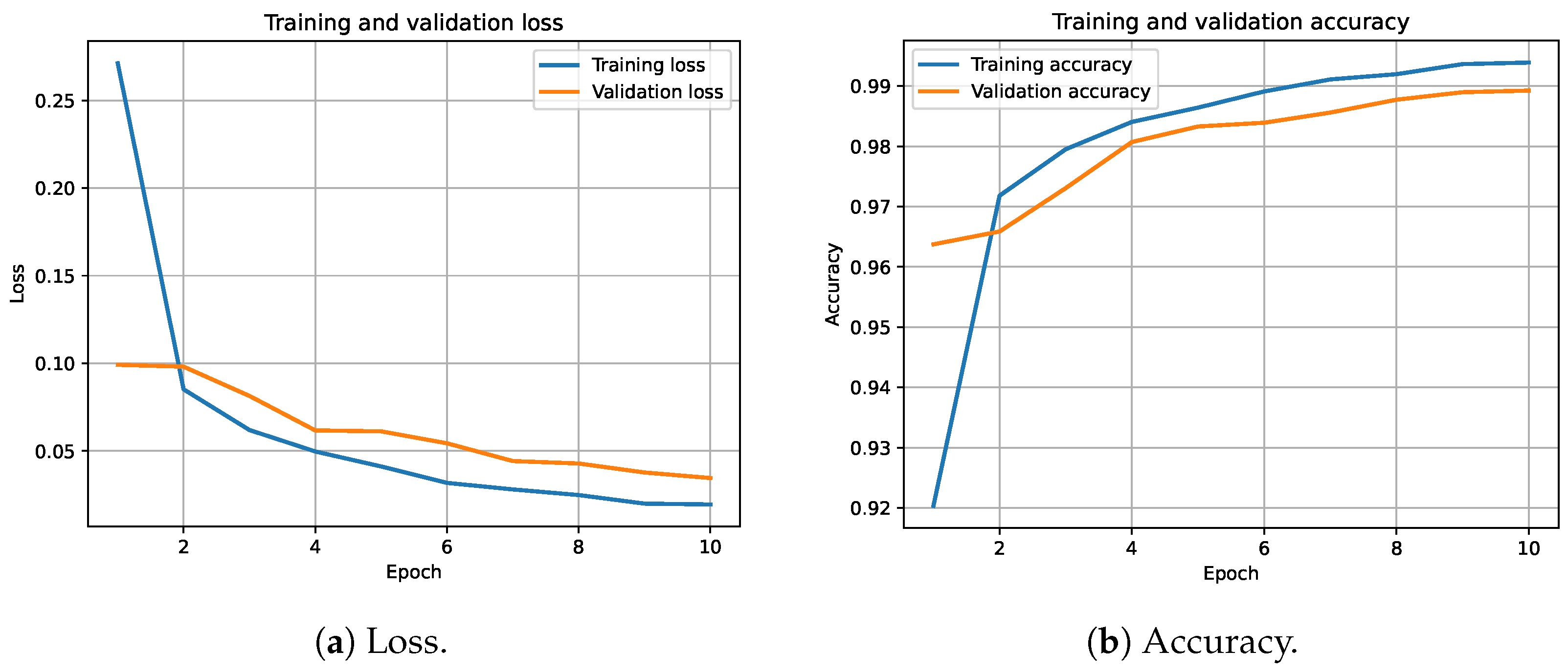
The proposed model has been trained on the considered dataset for 10 epochs by using 10% of the training set as the validation set (Python 3.10 source code can be downloaded from: https://github.com/mscarpiniti/CS-scalogram, accessed on 20 November 2023). The training and validation losses obtained during the training phase are shown in Figure 4a, while Figure 4b shows the corresponding training and validation accuracy. These figures demonstrate the effectiveness of the training, showing that the training procedure is quite stable after about seven epochs. Figure 4b also shows that, at convergence, the training accuracy is about 99.5%, while the validation one is about 99%.

Figure 4. Training and validation loss (a) and accuracy (b) of the proposed approach.

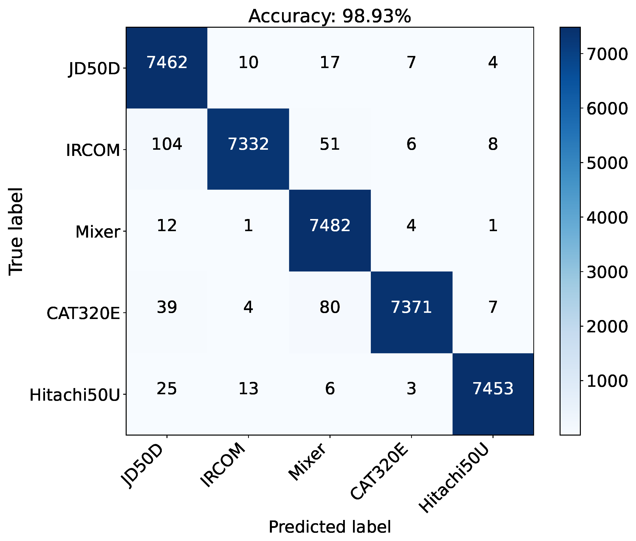
To evaluate the proposed approach, we have also used the overall accuracy, the per-class precision, the per-class recall, and the per-class F1-score, as well as their weighted averages [53], computed on the test set. Moreover, the confusion matrix is shown in Figure 5. The confusion matrix clearly shows that the proposed approach is able to provide very good results for the classification of real-world signals recorded in construction sites. In fact, most of the instances are in the main diagonal of the matrix. There is a little confusion between the compactor (IRCOM), which has been confused with the JD50D excavator and the concrete mixer, and the CAT320E excavator, which is, again, mainly confused with the JD50D excavator and the concrete mixer. This behavior is due to the fact that all of these pieces of equipment have similar engines.

Figure 5. Confusion matrix obtained by the proposed approach.

The results in terms of the precision, recall, and F1-score of the proposed approach are summarized in Table 3. In addition, this table confirms the conclusion drawn from the confusion matrix in Figure 5: the JD50D and Concrete Mixer classes have lower precision, while the compactor (IRCOM) and CAT320E excavator show lower recall. However, the F1-score is quite stable among all classes. The Hitachi 50U excavator performs the best in between the five considered classes. Despite this slight variability in performance, the weighted averages of the considered metrics are very good and settled at 0.989.

Table 3. Per-class performance of the proposed approach.

Class	Precision	Recall	F1-Score
JD50D	0.976	0.995	0.986
IRCOM	0.996	0.977	0.987
Mixer	0.979	0.998	0.988
CAT320E	0.997	0.983	0.989
Hitachi50U	0.997	0.994	0.996
All classes	0.989	0.989	0.989

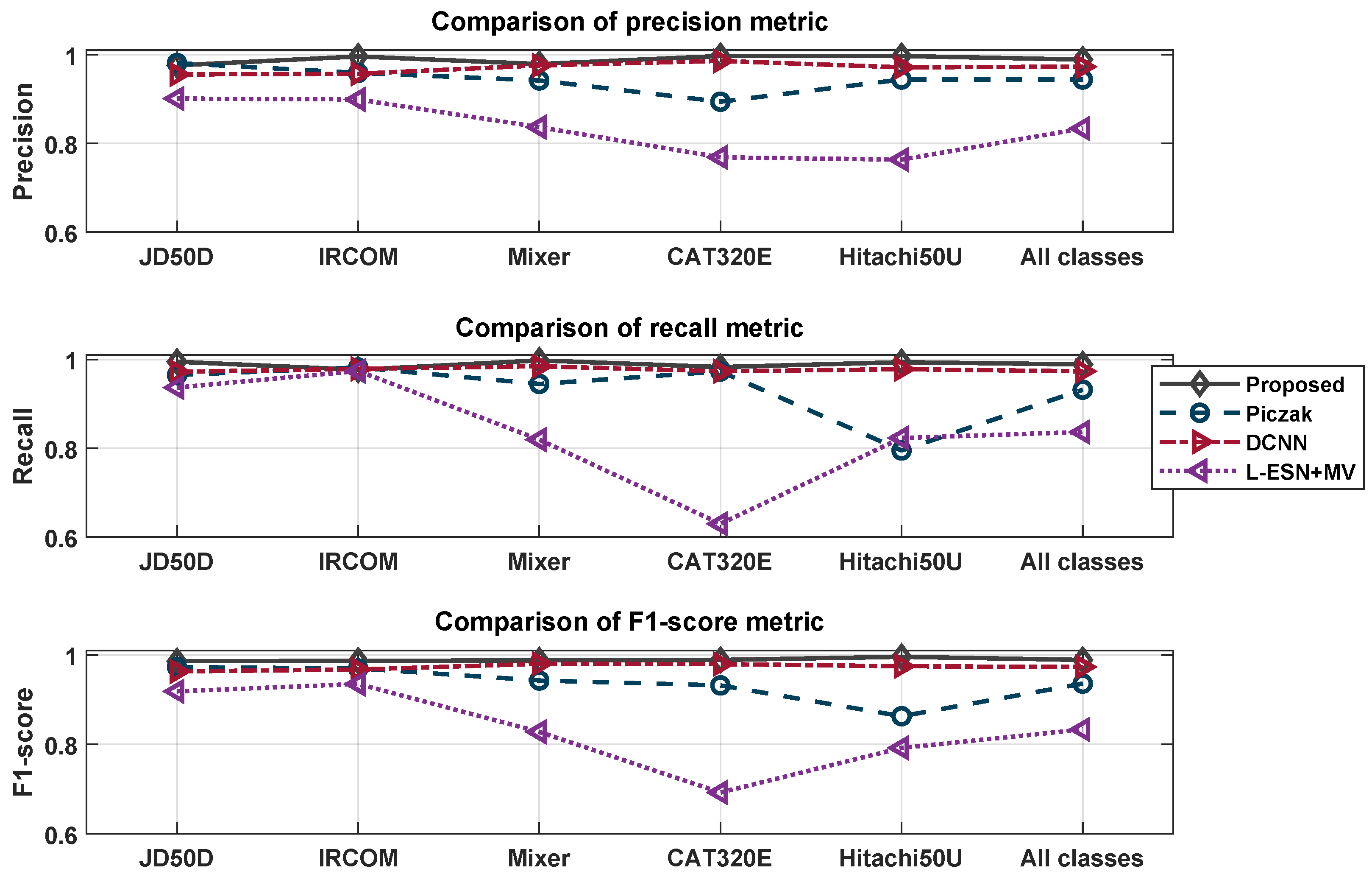
The proposed approach was compared with similar state-of-the-art solutions. Specifically, we compared our approach to the one proposed by Piczak in [4], based on a CNN fed by the spectrograms with corresponding deltas (i.e., the difference of the feature among two consecutive time instants); the approach proposed by Maccagno et al. in [31], based on a custom deep CNN (DCNN) fed by the spectrograms; and the approach proposed by Scarpiniti et al. in [34], based on an ESN working on several spectral features and a majority voting between adjacent chunks. The results obtained by these state-of-the-art approaches in terms of precision, recall, F1-score, and their weighted averages are shown in Table 4, Table 5, and Table 6, respectively. The results presented in these tables confirm that the approach proposed in this paper (see Table 3) performs better than the state of the art for all of the considered metrics. Figure 6 summarizes all of the considered metrics for these compared approaches.

Table 4. Per-class performance of the Piczak approach in [4].

Class	Precision	Recall	F1-Score
JD50D	0.981	0.965	0.973
IRCOM	0.959	0.982	0.970
Mixer	0.942	0.945	0.943
CAT320E	0.894	0.973	0.932
Hitachi50U	0.944	0.795	0.863
All classes	0.944	0.932	0.936

Table 5. Per-class performance of the DCNN-based approach in [31].

Class	Precision	Recall	F1-Score
JD50D	0.955	0.972	0.963
IRCOM	0.957	0.979	0.968
Mixer	0.975	0.985	0.980
CAT320E	0.986	0.973	0.979
Hitachi50U	0.972	0.978	0.975
All classes	0.973	0.973	0.973

Table 6. Per-class performance of the ESN-based approach in [34].

Class	Precision	Recall	F1-Score
JD50D	0.901	0.937	0.919
IRCOM	0.899	0.974	0.935
Mixer	0.837	0.819	0.828
CAT320E	0.769	0.629	0.692
Hitachi50U	0.763	0.823	0.792
All classes	0.834	0.837	0.833

Figure 6. A visual comparison of all the compared approaches for the precision (top), recall (middle), and F1-score (bottom).

In addition, Table 7 and Table 8 show the results of the works proposed by [44,46], which use scalogram-based approaches for acoustic scene classification. We adapt these approaches to work with the scalograms extracted from the construction site sounds. These tables show that, although the works proposed in [44,46] provide good results, the performance is slightly lower than the proposed approach reported in Table 3.

Table 7. Per-class performance of the approach proposed by Chen et al., 2018, in [44].

Class	Precision	Recall	F1-Score
JD50D	0.974	0.975	0.974
IRCOM	0.982	0.979	0.980
Mixer	0.981	0.984	0.982
CAT320E	0.988	0.979	0.984
Hitachi50U	0.975	0.983	0.979
All classes	0.980	0.980	0.980

Table 8. Per-class performance of the approach proposed by Copiaco et al., 2019, in [46].

Class	Precision	Recall	F1-Score
JD50D	0.972	0.973	0.972
IRCOM	0.981	0.977	0.979
Mixer	0.979	0.982	0.981
CAT320E	0.986	0.977	0.982
Hitachi50U	0.972	0.981	0.977
All classes	0.978	0.978	0.978

Although the Morlet wavelet in (4) is the most used and effective wavelet family in nonstationary audio analysis, we have also tested two other well-known and well-used wavelet families: the generalized Morse and the Bump wavelets [47], respectively. The results in terms of per-class precision, recall, and F1-score, and their related weighted averages, are shown in Table 9. From this table, we can argue that results of the generalized Morse wavelet are quite similar to those obtained by using the Morlet one (see Table 3). On the other hand, the results related to the Bump wavelet are slightly worse, even if they are quite good. The overall accuracies of these two approaches were 98.50% and 97.45%, respectively. These considerations confirm the effectiveness of the Morlet wavelet for analyzing audio signals in general and engine sounds in particular.

Table 9. Per-class performance of the proposed approach by using the generalized Morse wavelet and the Bump wavelet. Overall accuracy is 98.50% and 97.45%, respectively.

Class	Generalized Morse Wavelet			Bump Wavelet
	Precision	Recall	F1-Score	Precision	Recall	F1-Score
JD50D	0.985	0.977	0.981	0.964	0.983	0.974
IRCOM	0.986	0.983	0.985	0.990	0.967	0.978
Mixer	0.975	0.994	0.984	0.989	0.960	0.974
CAT320E	0.985	0.986	0.986	0.995	0.966	0.980
Hitachi50U	0.995	0.985	0.990	0.938	0.996	0.966
All classes	0.985	0.985	0.985	0.975	0.974	0.975

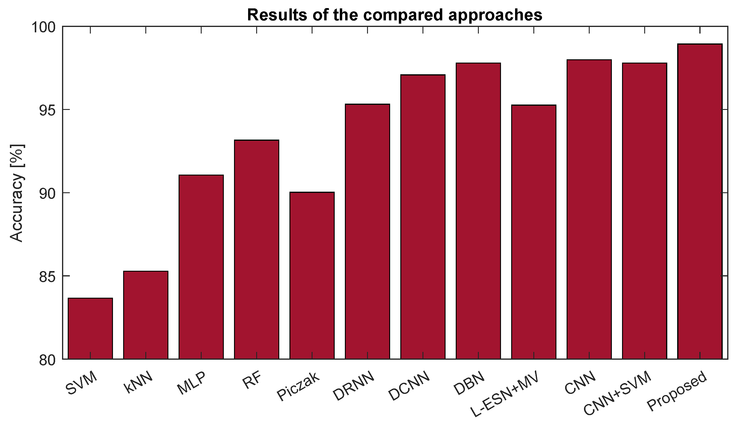
Finally, in Table 10, we summarize the previous results of the proposed approach (last row) and the compared ones by considering some additional machine learning and deep learning approaches. Specifically, Figure 7 shows the accuracy of the compared approaches as a bar plot. Among the machine learning techniques, we considered the results obtained by using a Support Vector Machine (SVM), the k-Nearest Neighbors (k-NN), the Multilayer Perceptron (MLP), and a random forest. All of these approaches provided reasonable results [5], though the results were worse than those provided by deep learning techniques. Among these last methods, we also considered an approach based on a Deep Recurrent Neural Network (DRNN) that exploits different spectral features [54] and one based on a Deep Belief Network (DBN) that works on a statistical ensemble of different spectral features [33]. For the implementation details, we refer to the related references. The results reported in Table 10 and Figure 7 clearly show once again the effectiveness of the proposed idea, which can be considered an effective and reliable approach for classifying real-world signals recorded in construction sites.

Table 10. Results of the compared approaches.

Approach	Accuracy	Precision	Recall	F1-Score
SVM [5]	83.66	0.846	0.838	0.842
k-NN [5]	85.28	0.860	0.853	0.857
MLP [5]	91.06	0.913	0.932	0.923
Random Forest [5]	93.16	0.934	0.932	0.933
Piczak [4]	90.03	0.944	0.932	0.936
DRNN [54]	95.32	0.955	0.953	0.954
DCNN [31]	97.08	0.973	0.973	0.973
DBN [33]	97.79	0.978	0.978	0.978
L-ESN+MV [34]	95.26	0.957	0.953	0.952
CNN [44]	97.99	0.980	0.980	0.980
CNN+SVM [46]	97.79	0.978	0.978	0.978
Proposed	98.93	0.989	0.989	0.989

Figure 7. Accuracy of the compared approaches.

As a discussion, we can observe that scalograms generally capture salient localized events in sound frames, as shown by the horizontal lines or cloud-like points in Figure 3. In addition, the convolutional layers of the CNN are able to learn discriminative features, as shown in Figure 8, which, for example, shows the 256 feature maps of the fifth and last convolutional layer of the used architecture. Although single plots in the figure are quite small, it is clear that feature maps in the final layer are more specialized in detecting specific time scales. In fact, the scalogram in Figure 8 shows clear horizontal lines localized at a specific scale. This kind of scale localization is typical of engines, a fundamental part of the machines considered in our dataset. This behavior justifies the better performance of the proposed approach for the classification of equipment sounds in construction sites.

Figure 8. The 256 feature maps of the fifth and last convolutional layer of the trained architecture. Maps have been normalized in $[0,1]$ for visualization: lighter colors are close to 1, while darker colors are close to 0.

8. Conclusions

In this paper, we have investigated the effectiveness of a Convolutional Neural Network (CNN) fed by scalograms in the classification of audio signals acquired in real-world construction sites. Specifically, after splitting the recorded signals into smaller chunks, the scalogram (i.e., the squared magnitude of the Continuous Wavelet Transform) has been computed and used as input to a customized version of the well-known AlexNet. The customization takes into account the single channel of the scalogram input and the reduced number of output classes. Some experimental results and comparisons with other state-of-the-art approaches confirm the effectiveness of the proposed idea, showing an overall accuracy of 98.9%.

In future work, we will investigate the effect of choosing different types of wavelet functions and the idea of early data fusion, i.e., by joining the scalograms with other bi-dimensional representations, such as the spectrogram or similar ones, and providing this augmented representation as the input to a CNN.