Prediction Modeling of Ground Subsidence Risk Based on Machine Learning Using the Attribute Information of Underground Utilities in Urban Areas in Korea

Abstract

As ground subsidence accidents in urban areas that occur due to damage to underground utilities can cause great damage, it is necessary to predict and prepare for such accidents in order to minimize such damage. It has been reported that the main cause of ground subsidence in urban areas is cavities in the ground formed by damage to underground utilities. Thus, in this study, attribute information and historical ground subsidence information of six types of underground utility lines (water supply, sewage, power, gas, heating, and communication) were collected to develop a ground subsidence risk prediction model based on machine learning. To predict the risk of ground subsidence in the target area, it was divided into a grid with a square size of 500 m × 500 m, and attribute information of underground utility lines and historical information of ground subsidence included in the grid were extracted. Six types of underground utility lines were merged into single-type attribute information, and the risk of ground subsidence was categorized into three levels using the number of ground subsidence occurrences to develop a dataset. In addition, 12 datasets, which were developed based on the conditions of certain divided ranges of attribute information and risk levels, and 12 additional datasets, which were developed using the Synthetic Minority Oversampling Technique to resolve the imbalance of data, were built. Then, factors that represented significant correlations between input and output data were singled out and were then applied to the RandomForest, XGBoost, and LightGBM algorithms to select a model that produced the best performance. By classifying the ground subsidence risk levels through the selected model, it was found that density was the most important influencing factor used in the model. A risk map of ground subsidence in the target area was made through the model; the map showed the trend of well-predicted risk levels in the area where ground subsidence was concentrated.

1. Introduction

Damage to underground utility lines is known to be one of the main causes of ground subsidence. Since underground utility lines are concentrated in urban areas with highly dense populations, accidents due to ground subsidence can cause significant social chaos [1]. As such, it is necessary to prevent accidents related to ground subsidence by analyzing their fundamental causes and mechanisms.

An investigation of the causes and the number of ground subsidence occurrences from 2010 to July 2014 in Seoul showed that the number of accidents has steadily increased, and their main cause was found to be damage to water supply and sewage lines [2]. A mechanism by which ground subsidence occurs is often when pipes are damaged by external impacts and deterioration due to aging, causing water channels to form around the damaged location. Soil particles in the ground can then move along the channels, creating and expanding cavities around the pipes [3]. Thus, ground subsidence is likely to increase as excavation construction work is repeatedly performed over time.

Extensive research has been performed on ways to prevent accidents related to ground subsidence. In Japan, a study using indoor model experiments simulating ground subsidence using standard sand was published to identify the mechanism of how cavities, a precursor to ground subsidence, were generated inside the ground, while a study on the identification of a cavity generation mechanism inside the ground by simulating a crack in the sewage pipeline under the soil box and visualization of the cavity generation through equipment such as X-rays and computed tomography has also been published [4,5].

Research that aims to identify the mechanism of ground subsidence occurrence using numerical analysis has also been active. Using the finite element method to simulate the ground cavity and relaxation zone, several published studies have shown that the location of the underground utility damage, the relative density of the ground, and the ground layer conditions have a significant effect on the ground subsidence [6,7,8].

In addition, studies on performing a decision tree, which is one of the machine learning algorithms, and the analytic hierarchy process, were published to derive factors influencing ground subsidence and calculate the weights of influencing factors [9,10].

Studies aiming to predict the risk level of ground subsidence have also been steadily conducted. One study on the evaluation of ground subsidence risk level that was announced uses surveyed CCTV data based on sewage pipelines, which is the main cause of ground subsidence, as well as cavity exploration data by underground exploration radar. In addition, a study was conducted to propose a regression equation of the ground subsidence risk level in urban areas in Korea through logistic regression analysis [11]. Moreover, studies have been conducted to select a model for predicting the ground subsidence risk level in urban areas in Korea through machine learning, after selecting influencing factors such as the number of years used and pipeline diameter among attribute values of underground utilities, and then to suggest a risk map [1].

Researchers have used various ways to predict risk levels in order to prevent accidents related to ground subsidence. However, they have had difficulty deriving highly accurate and reliable results, as ground subsidence occurs in complex ways and is caused by various factors in a wide range of areas. Thus, this study aims to propose a machine learning-based ground subsidence risk prediction model by selecting the following as influence factors among the attribute information of underground utility lines in representative urban areas in Korea: the number of years used, pipeline diameter and length, and the density of pipelines, which are likely to have a close correlation with ground subsidence. We compared the results of machine learning models by applying datasets with a range of conditions and selected the model that exhibited optimal performance. Furthermore, we aimed to present the importance of each influencing factor, which was used when classifying the ground subsidence risk levels by the machine learning model through the selected model.

2. Method and Data Characteristics

2.1. Subsection Flow of the Study

In this study, a representative urban area in Korea was selected as the target region. To develop a ground subsidence risk level prediction model based on machine learning, the historical information of ground subsidence, and attribute information of underground utility lines in the target region were used to build a dataset and then applied to the machine learning algorithm. The target region was divided into a grid with a total of 2391 squares of 500 m × 500 m in size, using the ArcGIS program to predict risk level. Six types of underground utility lines included in each grid square were merged into a single type to extract the attribute information and density. The dataset was built using a method that calculated a risk level based on the number of ground subsidence occurrences in the grid using the historical ground subsidence information.

The developed dataset was divided into training and test datasets at an 80:20 ratio to prevent overfitting of the model and to test the model. To mitigate the data imbalance, the Synthetic Minority Oversampling Technique (SMOTE) was applied to the training data. This developed training dataset was applied to machine learning algorithms: RandomForest (RF), XGBoost (XGB), and LightGBM (LGBM) to check the model results by adjusting the hyperparameters that exhibited the optimal performance. Using the 20% test data, the model’s performance was validated through the test indices of accuracy, F1-score, and area under the curve (AUC). Based on the test results, dataset types and machine learning models that exhibited optimal performance were selected, and the importance of the influencing factors was derived. Figure 1 shows the flow chart of the study.

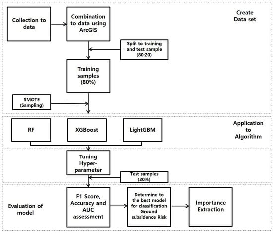
Figure 1. Flow chart.

2.2. Characteristics of the Data

A representative area in Korea was selected as the target region for the prediction of ground subsidence risk level. The target region was divided into a grid with a total of 2391 squares of 500 m × 500 m in size for the risk level evaluation. For each grid square, the attribute data of six types of underground utility lines (water supply, sewage, power, gas, heating, and communication cables) and the historical data of ground subsidence were compiled. As described above, six types of underground utility lines were merged into a single type to extract attribute data. In the attribute information of underground utility lines to build a dataset, the number of years used, pipeline type, diameter, length, burial depth, slope, etc., were included, but there were many missing and erroneous values as well. Thus, as the data that could be usable, the number of years used, pipeline diameter, and length were selected. Then, the density of all pipelines was calculated to be used as a factor influencing the occurrence of ground subsidence. To improve the model’s performance, raw data were not directly used, but they were preprocessed to divide the attribute information of underground utility lines by a certain range. The years used were divided into 5- and 10-year units, and the pipeline diameter was divided into 50 mm and 100 mm units. The basic unit of data that belongs to the corresponding range was set to the pipeline’s length. For example, an underground pipeline that was used for three years in the grid was assigned to a class corresponding to an age of 1 to 4 years, and the length of the pipeline was reflected.

For the output data, the risk level of ground subsidence was calculated by summing the number of ground subsidence occurrences in the grid using the historical information of ground subsidence occurrences. It is difficult to provide a quantifiable measure of ground subsidence risk. Thus, multiple datasets of ground subsidence risk levels, categorized by the number of ground subsidence occurrences, were developed. The developed datasets were applied to the machine learning algorithms to select a condition of the risk level of ground subsidence that exhibited good performance. The ground subsidence risk was categorized into three levels. Risk Level 1 means an area where the number of ground subsidence occurrences in the grid is “0”. The conditions of Risk Levels 2 and 3 were adjusted depending on the number of ground subsidence occurrences in the grid. If the number of ground subsidence occurrences in the grid of Risk Level 2 is one, the number of ground subsidence occurrences of Risk Level 3 was set to two or more. If the number of ground subsidence occurrences in the grid of Risk Level 2 is set to a range of one to two, the number of ground subsidence occurrences of Risk Level 3 was set to three or more. If the number of ground subsidence occurrences in the grid of Risk Level 2 is set to a range of one to three, the number of ground subsidence occurrences of Risk Level 3 was set to four or more. Risk Level 1 of ground subsidence means a relatively safer area from ground subsidence. The boundary between Levels 2 and 3 varies depending on the conditions, but Level 2 means an area that needs attention, and Level 3 is an area that is at the highest risk. Table 1 presents the categories of factors in the datasets. Table 2 presents the dataset which is set according to the data category condition. A total of 24 datasets were built according to whether or not SMOTE was applied to each dataset.

Table 1. Category of factors.

Factors	Unit	Category
Year (year)	5	1~5, 6~10, 11~15, 16~20, 21~25, 26~30, 31~35, 36~40, 41~45, 46~50
	10	1~10, 11~20, 21~30, 31~40, 41~50
Diameter (mm)	50	1~50, 51~100, 101~150, 151~200, 201~250, 251~300, 301~350, 351~400, 401~450, 451~500, 501~550, 551~600
	100	1~100, 101~200, 201~300, 301~400, 401~500, 501~600
Risk level (Sum of occurrences of ground subsidence in grid)	1	0
	2	1, 1~2, 1~3
	3	2~, 3~, 4~

Table 2. Category of Factors.

No.	Grid	Year (Year)	Diameter (mm)	Risk Level (Level 2′s Range)
1	500 m × 500 m	5	50	3 (1)
2				3 (1–2)
3				3 (1–3)
4			100	3 (1)
5				3 (1–2)
6				3 (1–3)
7		10	50	3 (1)
8				3 (1–2)
9				3 (1–3)
10			100	3 (1)
11				3 (1–2)
12				3 (1–3)

2.3. Density

A previous study proved that the density of pipelines was significantly correlated with ground subsidence [9] Accordingly, we used the density of the pipeline as the influencing factor of the model to predict the ground subsidence risk level. The density was calculated using a linear density analysis on the pipelines in the grid using ArcGIS. This method calculated the length of the pipeline that corresponded to the unit area.

2.4. Risk Level of Ground Subsidence

The risk levels used as the output data in this study were divided into three levels according to the number of times ground subsidence occurred in the grid. Since there are no quantifiable measures to categorize the risk level, we build datasets by selecting different numbers of data belonging to risk level 2 according to the number of occurrences of ground subsidence in the grid. Thus, the number of data varies according to the category based on the number of occurrences of ground subsidence of each dataset, which is presented in Table 3. As presented in Table 3, the ratio of Risk Level 1 data was the highest (57%), and the ratios of Risk Level 2 and 3 data varied according to the conditions. As such, the composition of the data shows unbalanced features, and we applied SMOTE, an over-sampling technique, to the 12 datasets to balance the data [12,13,14].

Table 3. The ratio of data according to the risk level of ground subsidence.

	Risk Level	1	2	3
Range of Risk Level 2
1		1374 (57%)	348 (15%)	669 (28%)
1–2		1374 (57%)	635 (27%)	382 (16%)
1–3		1374 (57%)	706 (30%)	311 (13%)

2.5. Data Correlation Analysis

A Pearson correlation analysis was conducted to verify the correlation between the input and output data of the dataset which was developed according to the data category conditions. The results are presented in Table 4.

Table 4. Results of correlation analysis of the influencing factors.

Model No.	1		2		3
Factor	Corr	p-Value	Corr	p-Value	Corr	p-Value
5Y_5	−0.138	0.000	−0.149	0.000	−0.150	0.000
5Y_10	−0.108	0.000	−0.098	0.000	−0.096	0.000
5Y_15	−0.004	0.858	−0.007	0.724	−0.049	0.017
5Y_20	−0.141	0.000	−0.178	0.000	−0.171	0.000
5Y_25	−0.108	0.000	−0.161	0.000	−0.154	0.000
5Y_30	−0.065	0.002	−0.099	0.000	−0.106	0.000
5Y_35	−0.150	0.000	−0.165	0.000	−0.173	0.000
5Y_40	−0.150	0.000	−0.169	0.000	−0.168	0.000
5Y_45	−0.167	0.000	−0.187	0.000	−0.167	0.000
5Y_50	−0.135	0.000	−0.134	0.000	−0.144	0.000
50DTR_50	0.057	0.005	0.061	0.003	0.064	0.002
50DTR_100	0.146	0.000	0.147	0.000	0.148	0.000
50DTR_150	0.159	0.000	0.163	0.000	0.169	0.000
50DTR_200	0.117	0.000	0.116	0.000	0.112	0.000
50DTR_250	0.015	0.478	0.008	0.698	0.013	0.522
50DTR_300	0.153	0.000	0.155	0.000	0.158	0.000
50DTR_350	0.038	0.067	0.026	0.198	0.022	0.274
50DTR_400	0.059	0.004	0.062	0.002	0.059	0.004
50DTR_450	0.099	0.000	0.109	0.000	0.107	0.000
50DTR_500	0.043	0.035	0.044	0.032	0.052	0.011
50DTR_550	0.014	0.494	−0.006	0.783	−0.003	0.895
50DTR_600	0.082	0.000	0.090	0.000	0.089	0.000
Density	0.544	0.000	0.534	0.000	0.526	0.000
Model No.	4		5		6
Factor	Corr	p-Value	Corr	p-Value	Corr	p-Value
5Y_5	−0.138	0.000	−0.149	0.000	−0.150	0.000
5Y_10	−0.108	0.000	−0.098	0.000	−0.096	0.000
5Y_15	−0.004	0.858	−0.007	0.724	−0.049	0.017
5Y_20	−0.141	0.000	−0.178	0.000	−0.171	0.000
5Y_25	−0.108	0.000	−0.161	0.000	−0.154	0.000
5Y_30	−0.065	0.002	−0.099	0.000	−0.106	0.000
5Y_35	−0.150	0.000	−0.165	0.000	−0.173	0.000
5Y_40	−0.150	0.000	−0.169	0.000	−0.168	0.000
5Y_45	−0.167	0.000	−0.187	0.000	−0.167	0.000
5Y_50	−0.135	0.000	−0.134	0.000	−0.144	0.000
100DTR_100	0.131	0.000	0.134	0.000	0.136	0.000
100DTR_200	0.152	0.000	0.154	0.000	0.155	0.000
100DTR_300	0.128	0.000	0.127	0.000	0.132	0.000
100DTR_400	0.067	0.001	0.064	0.002	0.060	0.004
100DTR_500	0.103	0.000	0.111	0.000	0.113	0.000
100DTR_600	0.083	0.000	0.089	0.000	0.088	0.000
Density	0.544	0.000	0.534	0.000	0.526	0.000
Model No.	7		8		9
Factor	Corr	p-Value	Corr	p-Value	Corr	p-Value
10Y_10	0.085	0.000	0.077	0.000	0.071	0.000
10Y_20	0.123	0.000	0.126	0.000	0.131	0.000
10Y_30	0.150	0.000	0.156	0.000	0.159	0.000
10Y_40	0.108	0.000	0.113	0.000	0.116	0.000
10Y_50	0.107	0.000	0.117	0.000	0.118	0.000
50DTR_50	0.057	0.005	0.061	0.003	0.064	0.002
50DTR_100	0.146	0.000	0.147	0.000	0.148	0.000
50DTR_150	0.159	0.000	0.163	0.000	0.169	0.000
50DTR_200	0.117	0.000	0.116	0.000	0.112	0.000
50DTR_250	0.015	0.478	0.008	0.698	0.013	0.522
50DTR_300	0.153	0.000	0.155	0.000	0.158	0.000
50DTR_350	0.038	0.067	0.026	0.198	0.022	0.274
50DTR_400	0.059	0.004	0.062	0.002	0.059	0.004
50DTR_450	0.099	0.000	0.109	0.000	0.107	0.000
50DTR_500	0.043	0.035	0.044	0.032	0.052	0.011
50DTR_550	0.014	0.494	−0.006	0.783	−0.003	0.895
50DTR_600	0.082	0.000	0.090	0.000	0.089	0.000
Density	0.544	0.000	0.534	0.000	0.526	0.000
Model No.	10		11		12
Factor	Corr	p-Value	Corr	p-Value	Corr	p-Value
10Y_10	0.085	0.000	0.077	0.000	0.071	0.000
10Y_20	0.123	0.000	0.126	0.000	0.131	0.000
10Y_30	0.150	0.000	0.156	0.000	0.159	0.000
10Y_40	0.108	0.000	0.113	0.000	0.116	0.000
10Y_50	0.107	0.000	0.117	0.000	0.118	0.000
100DTR_100	0.131	0.000	0.134	0.000	0.136	0.000
100DTR_200	0.152	0.000	0.154	0.000	0.155	0.000
100DTR_300	0.128	0.000	0.127	0.000	0.132	0.000
100DTR_400	0.067	0.001	0.064	0.002	0.060	0.004
100DTR_500	0.103	0.000	0.111	0.000	0.113	0.000
100DTR_600	0.083	0.000	0.089	0.000	0.088	0.000
Density	0.544	0.000	0.534	0.000	0.526	0.000

In Table 4, Y refers to the number of years used, and 5Y and 10Y mean the five-year and 10-year units, respectively (5–50 refers to the data range). In addition, DTR refers to the pipeline diameter; 50 and 100 refer to the pipeline diameter of 50 mm and 100 mm, and 50–600 refers to the range of the pipeline diameters. In this study, the presence of data correlation was verified by p-value in the correlation analysis. If the p-value was less than 0.05, it was interpreted as showing a significant correlation, so it was used as input data. Conversely, if the p-value is more than 0.05, it was interpreted as not showing a significant correlation, so it was excluded from the input data.

3. Results of Analysis of Ground Subsidence Risk Levels Using Machine Learning

In this study, a machine learning algorithm was used to develop a model to predict the risk level of ground subsidence, focusing on urban areas in South Korea. The machine learning algorithms used were RF, XGB, and LGBM, which have produced good results in previous studies [1,15].

3.1. Random Forest

The Random Forest (RF) algorithm is a tree-based ensemble model that is developed to solve regression and classification problems in machine learning [16]. An ensemble model derives better results than a model that trains a single model once, as it trains multiple algorithms iteratively. It includes techniques such as voting and bagging.

RF presents the best result among the results derived from the trees after creating multiple tree-based algorithms as the representative result. RF is based on a tree algorithm, has a low overfitting risk, and can be easily applied to various data. It is widely used in problem-solving through machine learning to derive a good result [17,18,19,20].

RF predicts the outcome as a binary value of 0 or 1, as presented in (1), after extracting an arbitrary number of input data from a number of single-algorithm predictors and performing a final decision by majority vote on the results derived from each predictor, where $y_i=f_i\left(\mathrm{X}\right)$, and $w_i$ refers to the weight. If the calculated value is larger than the threshold value, the predicted value is 1, otherwise it is 0 [21].

$$\mathrm{F}\left(\mathrm{X}\right)=\sum w_i{y}_i$$

(1)

3.2. XGBoost (eXtreme Gradient Boosting)

XGBoost (XGB) is a typical algorithm of a boosting technique where a result is derived by learning a single model sequentially, and the result of the previous model affects the next result. XGB is a tree-based algorithm used in solving regression and classification problems. It is effective in preventing overfitting due to its different regularization penalties. In addition, it has the advantage of being able to process big data in a short period of time, so it has been actively used in various fields [22,23].

The calculation equation for the decision-making of XGBoost is presented in (2), where $\widehat{y_i}$ refers to the i-th sample’s prediction value and $f_k$ refers to the prediction value where the k-th tree’s sigmoid function is applied. The output is derived by summing all prediction values. The prediction value can be calculated using (3).

$${\widehat{y}}_i={\sum }_{K=1}^K{f}_i\left(x_i\right)$$

(2)

$${\widehat{y}}_i=\frac{1}{1+e^{-f\left(x_i\right)}}$$

(3)

The error is calculated using the difference between the prediction and real values in the tree, and the weight is calculated to reduce the error as presented in (4). ${\widehat{y_i}}^{\left(t-1\right)}$ refers to the prediction value of the previous model, $h_t\left(x_i\right)$ refers to the tree trained by the current model, and $\eta$ refers to the learning rate, which is the percentage of reflections from the prior model. The model’s error is reduced by iterating this method [24,25].

$${\widehat{y}}_i^{\left(t\right)}={\widehat{y}}_i^{\left(t-1\right)}+\eta h_t(x_i)$$

(4)

3.3. LightGBM (Light Gradient Boosting Machine)

LightGBM (LGBM) is an algorithm in which a tree-based boosting technique is applied in the same manner as XGB. It has been used in solving regression and classification problems and in selecting the priority of importance of influencing factors. LGBM is advantageous for its fast operation speed because it derives a result using a method that reduces data characteristics by employing partial data only. Thus, LGBM processes big data quickly and with a high level of accuracy, and can derive the importance among the influencing factors used, advantages which have made it a popular choice [26].

LightGBM calculates the loss function using cross-entropy. The equation for calculating the cross-entropy is presented in (5), where N is the number of samples, K is the number of classes, $y_{i,j}$ refers to the binary variable indicating whether the i-th sample belongs to the j-th class, and $p_{i,j}$ refers to the probability that the i-th sample belongs to the j-th class. LightGBM derives its results by learning to update the model while minimizing the CE received from the previous model [27].

$$\mathrm{CE}=\frac{1}{N}{\sum }_{i=1}^N{\sum }_{j=1}^N{y}_{i,j}\log \left(p_{i,j}\right)$$

(5)

3.4. Evaluation Indexes of Machine Learning Algorithms

For evaluation indexes of machine learning models to solve a classification problem, accuracy, F1-score, and AUC are generally used. The results of these evaluation indexes can be calculated using Equations (6)–(10) via the confusion matrix.

$$\mathrm{Accuracy}=\frac{\mathrm{TP}+\mathrm{TN}}{\mathrm{TP}+\mathrm{TN}+\mathrm{FP}+\mathrm{FN}}$$

(6)

$$\mathrm{Recall}\left(\mathrm{Sensitivity}\right)=\frac{\mathrm{TP}}{\mathrm{TP}+\mathrm{FN}}$$

(7)

$$\mathrm{Precision}=\frac{\mathrm{TP}}{\mathrm{TP}+\mathrm{FP}}$$

(8)

$$\mathrm{F}1\mathrm{Score}=2\times \frac{\mathrm{Precision}\times \mathrm{Recall}}{\mathrm{Precision}+\mathrm{Recall}}$$

(9)

$$\mathrm{Specificity}=\frac{\mathrm{TN}}{\mathrm{TN}+\mathrm{FP}}$$

(10)

Intuitively, it is highly convenient if the model’s performance is evaluated through the model’s accuracy, but it is also difficult to identify the objective model performance for imbalanced data. Thus, a model using imbalanced data is evaluated by employing the F1-score, which uses a harmonic mean of the data. The model confidence is evaluated using the AUC that uses the receiver operation characteristic (ROC) [28,29,30,31,32,33,34].

3.5. Results of Applying Machine Learning

To build a machine learning-based model for the prediction of ground subsidence risk levels in urban areas, we selected a model that exhibited the best performance by applying 24 datasets, which were developed using the attribute information of underground utility lines and the historical information of ground subsidence, to RF, XGB, and LGBM classifiers. To implement machine learning, Python 3.8 was used, and the Scikit-learn library was employed.

The model’s evaluation indexes, accuracy, F1-score, and AUC were selected. The accuracy was used to determine the presence of overfitting by comparing the results of the training set with those of the test set. If the difference between the training and test scores is equal to or less than 0.1, it was determined that overfitting was avoided. In addition, the model’s performance was identified using the F1-score and AUC indices to select the optimal model.

The results of an evaluation of the machine learning models derived in this study are presented in Table 5 and Table 6. Table 5 shows the model results where SMOTE was not applied, and Table 6 presents the model results where SMOTE was applied.

Table 5. Results of machine learning model (SMOTE not applied).

Model	RF				XGB				LGBM
No.	Train Score	Test Score	F1-Score (Macro)	AUC (Macro)	Train Score	Test Score	F1-Score (Macro)	AUC (Macro)	Train Score	Test Score	F1-Score (Macro)	AUC (Macro)
1	0.742	0.670	0.450	0.780	0.725	0.668	0.480	0.770	0.765	0.676	0.480	0.800
2	0.766	0.645	0.500	0.800	0.719	0.628	0.490	0.790	0.714	0.666	0.550	0.800
3	0.745	0.649	0.490	0.810	0.768	0.660	0.560	0.800	0.759	0.643	0.560	0.810
4	0.791	0.676	0.470	0.780	0.724	0.674	0.490	0.770	0.763	0.670	0.480	0.790
5	0.764	0.664	0.530	0.800	0.719	0.628	0.500	0.790	0.758	0.660	0.550	0.810
6	0.751	0.664	0.520	0.810	0.732	0.658	0.550	0.810	0.768	0.666	0.570	0.820
7	0.736	0.639	0.420	0.750	0.696	0.641	0.410	0.750	0.714	0.645	0.440	0.750
8	0.681	0.591	0.310	0.750	0.694	0.601	0.390	0.750	0.655	0.591	0.360	0.760
9	0.732	0.635	0.390	0.770	0.680	0.620	0.410	0.770	0.715	0.616	0.410	0.770
10	0.729	0.643	0.430	0.740	0.697	0.647	0.420	0.740	0.715	0.635	0.420	0.750
11	0.651	0.597	0.330	0.750	0.686	0.599	0.380	0.740	0.681	0.603	0.360	0.750
12	0.729	0.635	0.400	0.770	0.683	0.599	0.350	0.760	0.706	0.610	0.350	0.760

Table 6. Results of machine learning model (SMOTE applied).

Model	RF				XGB				LGBM
No.	Train Score	Test Score	F1-Score (Macro)	AUC (Macro)	Train Score	Test Score	F1-Score (Macro)	AUC (Macro)	Train Score	Test Score	F1-Score (Macro)	AUC (Macro)
1	0.676	0.626	0.560	0.790	0.648	0.608	0.560	0.770	0.716	0.628	0.560	0.790
2	0.683	0.593	0.550	0.790	0.705	0.608	0.580	0.800	0.656	0.593	0.560	0.800
3	0.718	0.608	0.550	0.790	0.744	0.644	0.590	0.800	0.706	0.620	0.570	0.810
4	0.662	0.624	0.560	0.790	0.679	0.585	0.510	0.770	0.656	0.582	0.520	0.790
5	0.687	0.595	0.560	0.800	0.666	0.587	0.550	0.790	0.690	0.597	0.550	0.800
6	0.699	0.585	0.540	0.800	0.712	0.612	0.560	0.800	0.729	0.624	0.570	0.820
7	0.671	0.603	0.530	0.760	0.655	0.580	0.520	0.770	0.668	0.580	0.520	0.770
8	0.645	0.543	0.460	0.750	0.615	0.553	0.500	0.740	0.655	0.545	0.490	0.750
9	0.632	0.501	0.380	0.740	0.628	0.553	0.490	0.770	0.627	0.551	0.490	0.760
10	0.682	0.597	0.520	0.770	0.660	0.578	0.520	0.760	0.669	0.578	0.510	0.770
11	0.608	0.541	0.450	0.750	0.647	0.555	0.490	0.740	0.651	0.570	0.500	0.750
12	0.636	0.511	0.390	0.750	0.615	0.532	0.460	0.760	0.676	0.568	0.490	0.750

Based on the evaluation results, the optimal model for the prediction of ground subsidence risk levels in the target region was determined. It was SMOTE-applied XGB (No. 3 model) when the number of years used was a five-year unit, the pipeline diameter was 50mm, and the number of ground subsidence occurrences in the grid of risk level 2 was set to 1 to 3. In this model, the F1-score (0.590) and AUC (0.800) were the best, and the difference between the training (0.744) and test (0.644) scores was equal to or less than 0.1, which meant overfitting was avoided. Thus, this model was selected as the fittest classifier for the prediction model of ground subsidence risk level in the target region.

The model results, according to whether or not SMOTE was applied, revealed that when SMOTE was not applied there was an F1-score of 0.310 to 0.570, and when SMOTE was applied there was an F1-score of 0.380 to 0.590. This meant that the imbalance in the number of ground subsidence occurrences, which was the output data, was resolved through SMOTE, thereby obtaining an efficient classification of the model. F1-Score and AUC of the XGB classifier in this study were 0.590 and 0.8 (Figure 2). Thus, XGB was found to not be a very good model from a computer science perspective. This result is due to the deepening of the data imbalance caused by the wide range of target areas and the limited use of influencing factors (underground utility attribute information). As ground subsidence is a phenomenon caused by various causes (underground structures, ground conditions, ground layer, etc.) in addition to the damage to underground utility lines, it is expected that the performance of the model will be improved in the future by obtaining more data on the underground space.

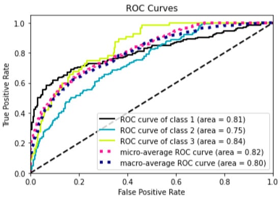
Figure 2. ROC Curves of XGB Model.

In addition, the tuning of the hyperparameters of each classifier was set to the hyperparameter that produces the optimal result using a trial-and-error method. Table 7 summarizes the main hyperparameters of the selected XGB model.

Table 7. Summary of hyperparameters in the model.

Model	Hyper Parameter
XGB	Estimators (300), learning rate (0.002), max depth (4)

The XGB model included a function to derive the importance of the input data employed in the process of solving the classification problem. Using this function, we selected the main influencing factors used to classify the ground subsidence risk levels. Figure 3 shows a graph that exhibits the importance of the factors used in the model, in which Y refers to the number of years used and DTR refers to the pipeline diameter. Density was the most importantly used factor in the classification of ground subsidence risk levels in the XGB model. The number of years used was found to be more important than the diameter of the pipeline. In pipelines used between 20 and 40 years, it was found to be relatively more important.

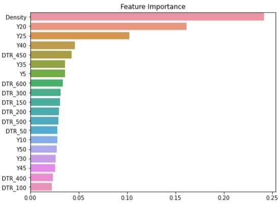
Figure 3. Importance of influencing factors in the XGB model.

3.6. Map of Ground Subsidence Risk

Figure 4 shows a prediction map of the ground subsidence risk level in the target region using the selected prediction model of ground subsidence risk level, as well as a map of ground subsidence risk level based on the historical data of past ground subsidence. In the Figure, the red, yellow, and green colors refer to Level 3, Level 2, and Level 1 ground subsidence risk, respectively. The points on the map indicate the regions where ground subsidence occurred.

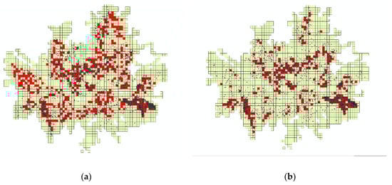
Figure 4. Map of ground subsidence risk. (a) Prediction map of ground subsidence risk level. (b) Map of ground subsidence risk using real data.

When comparing the prediction map using the model and the map drawn based on the past ground subsidence data, the prediction map had relatively higher risk levels. The prediction model classified the region in which ground subsidence was concentrated in the past as the high-risk region. The prediction map of ground subsidence risk levels in the region will be used as a basis for the management entity to prioritize the areas to be inspected when investigating cavities inside the ground for the prevention of ground subsidence.

4. Conclusions

To develop a model that predicts the risk level of ground subsidence and create a risk level map targeting the urban area in South Korea, a dataset was built using the pipeline length, the number of years used, and the diameter and density of pipelines in the target area. The developed datasets were applied to machine learning algorithms RF, XGB, and LGBM, to comparatively analyze the evaluation indexes. Through this process, the best performance was found in the model with the following dataset conditions applied to the XGB classifier: the number of years used was five years, the pipeline diameter was 50 mm, and the number of ground subsidence occurrences in the grid with risk Level 2 of ground subsidence was set to 1 to 3, when using SMOTE applied data (F1 Score = 0.590, AUC = 0.8). Previously, a machine learning-based ground subsidence risk prediction model has been developed for a small subset of urban areas (two districts) in South Korea [15]. However, since the model was trained using data from a very small area, it is not reliable enough to be applied to a wide range of target areas. Thus, in this study, we collected a large number of data for the entire city and proposed a model for predicting the risk of ground subsidence. As a result, it is now possible to create a reliable ground subsidence risk map for urban areas in Korea through the ground subsidence risk prediction model presented in this study.

The ground subsidence risk prediction model presented in this study derives the importance of influencing factors used when classifying the risk level of ground subsidence. Our study results verified that the density had the highest importance, and the number of years used was more important than the pipeline diameter. This result is similar to that of a previous study which found the density and the number of ground subsidence occurrences were highly correlated [9], as well as another study where the aging of pipelines had an impact on the ground subsidence occurrence as the number of years used increased [3]. Thus, excavation work to bury underground utility lines should be minimized, and aged pipelines should be managed to cope with ground subsidence.

The risk level map of ground subsidence in the target area was created using the ground subsidence risk prediction model. This map predicted a number of spots with higher risk levels than that in the risk map based on the historical data of past ground subsidence. The ground subsidence risk prediction classifier presented in this study predicted the risk level of the area in which ground subsidence was concentrated in the past relatively well.

It is expected that the results presented in this study can be used as foundational data for a proactive response to the occurrence of ground subsidence in urban areas. In future research, we will add underground structures (subway tunnels, etc.) and high-rise building information in the target region to develop a more reliable prediction model of ground subsidence risk level in urban areas.

References

- Lee, S.Y.; Kang, J.M.; Kim, J.Y. Development of Machine Learning Model to predict the ground subsidence risk grade according to the Characteristics of underground facility. J. Korean Geo-Environ. Soc. 2022, 23, 5–10. [Google Scholar]
- Seoul city, Cause Analysis of Cavity at Seokchon Underground Roadway and Road Cavity, Seokchon-dong Cavity Cause Investigation Committee. 2014.
- Kim, J.Y.; Kang, J.M.; Choi, C.H.; Park, D.H. Correlation Analysis of Sewer Integrity and Ground Subsidence. J. Korean Geo-Environ. Soc. 2017, 18, 31–37. [Google Scholar]
- Kuwano, R.; Horii, T.; Kohashi, H.; Yamauchi, K. Defects of sewer pipes causing cave-in’s in the road. In Proceedings of the 5th International Symposium on New Technologies for Urban Safety of Mega Cities in Asia, Phuket, Thailand, 16–17 November 2006; pp. 347–353. [Google Scholar]
- Mukunoki, T.; Kuwano, N.; Otani, J.; Kuwano, R. Visualization of three dimensional failure in sand due to water inflow and soil drainage from defected underground pipe using X-ray CT. Soils Found. 2009, 49, 959–968. [Google Scholar] [CrossRef]
- Masud, M.; Bairagi, A.K.; Nahid, A.A.; Sikder, N.; Rubaiee, S.; Ahmed, A.; Anand, D. A Pneumonia Diagnosis Scheme Based on Hybrid Features Extracted from Chest Radiographs Using an Ensemble Learning Algorithm. J. Healthc. Eng. 2021, 2021, 11. [Google Scholar] [CrossRef] [PubMed]
- Takeuchi, D.; Fukatani, W.; Miyamoto, T.; Yokota, T. Using decision tree analysis to extract factors affecting road subsidence. J. Jpn. Sew. Work. Assoc. 2007, 54, 124–133. [Google Scholar]
- Jin, Y.S. The Analysis on Correlation of Precipitation and Risk Factors to the Soil Subsidence. Ph.D. Dissertation, Chonnam National University, Gwangju, Republic of Korea, 2018; pp. 104–105. [Google Scholar]
- Kim, K.Y. Susceptibility Model for Sinkholes Caused by Damaged Sewer Pipes Based on Logistic Regression. Master’s Thesis, Seoul National University, Seoul, Republic of Korea, 2018. [Google Scholar]
- Han, M.S. A Risk Assessment of Ground Subsidence by GPR and CCTV Investigation. Master’s Thesis, Seoul National University of Science and Technology, Seoul, Republic of Korea, 2017. [Google Scholar]
- Kim, J.Y.; Kang, J.M.; Choi, C.H. Correlation Analysis of the Occurrence of Ground Subsidence According to the Density of Underground Pipelines. J. Korean Geo-Environ. Soc. 2021, 22, 23–29. [Google Scholar]
- Muhammad, F.I.; Ganjar, A.; Muhammad, S.; Rhee, J. Hybrid Prediction Model for Type 2 Diabetes and Hypertension Using DBSCAN-Based Outlier Detection, Synthetic Minority Over Sampling Technique (SMOTE), and Random Forest. Appl. Sci. 2018, 8, 1325. [Google Scholar] [CrossRef]
- Mimi, M.; Matloob, K. SMOTE-ENC: A Novel SMOTE-Based Method to Generate Synthetic Data for Nominal and Continuous Features. Appl. Syst. Innov. 2021, 4, 18. [Google Scholar] [CrossRef]
- Georgios, D.; Fernado, B.; Joao, F.; Manvel, K. Imbalanced Learning in Land Cover Classification: Improving Minority Classes’ Prediction Accuracy Using the Geometric SMOTE Algorithm. Remote Sens. 2019, 11, 3040. [Google Scholar] [CrossRef]
- Lee, S.Y.; Kang, J.M.; Kim, J.Y. Ground Subsidence Risk Grade Prediction Model Based on Machine Learning According to the Underground Facility Properties and Density. J. Korean Geo-Environ. Soc. 2023, 24, 23–29. [Google Scholar]
- Breiman, L.; Friedman, J.; Stone, C.; Olshen, R. Classification and Regression Trees; Taylor & Francis: Abingdon, UK, 1984. [Google Scholar]
- Pal, M. Random forest classifier for remote sensing classification. Int. J. Remote Sens. 2005, 26, 217–222. [Google Scholar] [CrossRef]
- Park, E.J.; Park, J.H.; Kim, H.H. Mapping Species-Specific Optimal Plantation Sites Using Random Forest in Gyeongsangnam-do Province, South Korea. J. Agric. Life Sci. 2019, 53, 65–74. [Google Scholar] [CrossRef]
- Hastie, T.; Tibshirani, R.; Friedman, J. The Elements of Statistical Learning: Data Mining, Inference, and Prediction, 2nd ed.; Springer: Berlin/Heidelberg, Germany, 2009; p. 745. [Google Scholar]
- Lee, S.H.; Yoon, Y.A.; Jung, J.H.; Sim, H.S.; Chang, T.W.; Kim, Y.S. A Machine Learning Model for Predicting Silica Concentrations through Time Series Analysis of Mining Data. J. Korean Soc. Qual. Manag. 2020, 48, 511–520. [Google Scholar]
- Louppe, G. Understanding Random Forests; University of Liege: Liege, Belgium, 2014; p. 211. [Google Scholar]
- Chen, T.; Guestrin, C. XGBoost: A Scalable Tree Boosting System, KDD’16. In Proceedings of the 22nd ACM SIGKDD International Conference on Knowledge Discovery and Data Mining, San Francisco, CA, USA, 13–17 August 2016; pp. 785–794. [Google Scholar]
- Zhang, Y.; Haghani, A. A gradient boosting method to improve travel time prediction. Transportation Research Part C. Emerg. Technol. 2015, 58, 308–324. [Google Scholar] [CrossRef]
- Zhang, D.; Chen, H.D.; Zulfiqar, H.; Yuan, S.S.; Huang, Q.L.; Zhang, Z.Y.; Deng, K.J. iBLP: An XGBoost-Based Predictor for Identifying Bioluminescent Proteins. Comput. Math. Methods Med. 2021, 2021, 15. [Google Scholar] [CrossRef]
- Le NQ, K.; Do, D.T.; Le, Q.A. A sequence-based prediction of Kruppel-like factors proteins using XGBoost and optimized features. Gene 2021, 787, 145643. [Google Scholar] [CrossRef]
- Ke, G.; Meng, Q.; Finley, T.; Wang, T.; Chen, W.; Ma, W.; Ye, Q.; Liu, T. LightGBM: A Highly Efficient Gradient Boosting Decision Tree, Part of Advances in Neural Information Processing Systems. Adv. Neural Inf. Process. Syst. 2017, 30, 1. [Google Scholar]
- Lv, J.; Wang, C.; Gao, W.; Zhao, Q. An Economic Forecasting Method Based on the LightGBM-Optimized LSTM and Time-Series Model. Comput. Intell. Neurosci. 2021, 2021, 10. [Google Scholar] [CrossRef]
- Sokolova, M.; Japkowicz, N.; Szpakowicz, S. Beyond Accuracy, F-Score and ROC: A Family of Discriminant Measures for Performance Evaluation. In Proceedings of the Advances in Artificial Intelligence (AI 2006) Lecture Notes in Computer Science; Springer: Heidelberg, Germany, 2006; Volume 4304, pp. 1015–1021. [Google Scholar]
- Wang, L.; Chu, F.; Xie, W. Accurate cancer classification using expressions of very few genes. IEEE/ACM Trans. Comput. Biol. Bioinf. 2007, 4, 40–53. [Google Scholar] [CrossRef]
- Gu, Q.; Zhu, L.; Cai, Z. Evaluation measures of the classification performance of imbalanced data sets. In Proceedings of the ISICA 2009—The 4th International Symposium on Computational Intelligence and Intelligent Systems, Communications in Computer and Information Science, Huangshi, China, 23–25 October 2009; Springer: Heidelberg, Germany, 2009; Volume 51, pp. 461–471. [Google Scholar]
- Bekkar, M.; Djemaa, H.K.; Alitouche, T.A. Evaluation measures for models assessment over imbalanced data sets. J. Inf. Eng. Appl. 2013, 3, 27–38. [Google Scholar]
- Akosa, J.S. Predictive accuracy: A misleading performance measure for highly imbalanced data. In Proceedings of the SAS Global Forum 2017 Conference, Orlando, FL, USA, 2–5 April 2017; SAS Institute Inc.: Cary, NC, USA, 2017; pp. 942–2017. [Google Scholar]
- Davide, C.; Giuseppe, J. The advantages of the Matthews correlation coefficient (MCC) over F1 score and accuracy in binary classification evaluation. BMC Genom. 2020, 21, 6. [Google Scholar]
- Nguyen, Q.K.L.; Nguyen, T.T.D.; Ou, Y.Y. Identifying the molecular functions of electron transport proteins using radial basis function networks and biochemical properties. J. Mol. Graph. Model. 2017, 73, 166–178. [Google Scholar]
Disclaimer/Publisher’s Note: The statements, opinions and data contained in all publications are solely those of the individual author(s) and contributor(s) and not of MDPI and/or the editor(s). MDPI and/or the editor(s) disclaim responsibility for any injury to people or property resulting from any ideas, methods, instructions or products referred to in the content. |
© 2023 by the authors. Licensee MDPI, Basel, Switzerland. This article is an open access article distributed under the terms and conditions of the Creative Commons Attribution (CC BY) license (https://creativecommons.org/licenses/by/4.0/).