Adaptive Cruise Control Strategy for Electric Vehicles Considering Battery Degradation Characteristics

Abstract

This paper proposes an economic adaptive cruise controller (EACC) that considers battery aging characteristics based on adaptive model predictive control (AMPC). By establishing a battery capacity decay model based on experimental data, the capacity loss during vehicle operation is determined, and the parameters in the equivalent circuit model are updated according to the actual capacity of the battery. The controller uses indicators that characterize driving safety, tracking performance, comfort, and economy. The economic indicator is the decrease in the value of the battery capacity. Fuzzy weight allocation is designed based on the host vehicle’s speed and the workshop’s relative distance to adjust the weight between different indicators under different working conditions. Additionally, the proposed controller is compared with other traditional controllers under different working conditions, cycle times, and battery state of health (SOH). The simulation results indicate that, under various battery SOH conditions, the performance of the controller which considers battery capacity degradation characteristics is better than that of traditional controllers. Moreover, the fixed-weight controller performs better when following a vehicle at medium and low speeds. Finally, the proposed strategy was validated through hardware-in-the-loop testing, demonstrating its ability to meet the real-time requirements of the system.

1. Introduction

With the continuous development of the automotive industry, after consumers’ daily travel needs have been satisfied they pay more attention to the driving performance of cars [1]. Today, autonomous driving has become the focus of attention [2]. In order to realize this function, the body of development work carried out by the automotive industry has gradually shifted from fuel vehicles to new energy vehicles, and electrified and intelligent electric vehicles stand out as the main research goal at present [3]. The adaptive cruise control (ACC) system is one of the advanced driver assistance systems. As a key step in achieving autonomous vehicle driving [4], it can not only reduce the probability of accidents caused by driver misuse [5] and improve driving safety, but also design driving strategies that match the road conditions at any given time [6]. ACC-equipped vehicles use on-board sensors to understand the position and speed of surrounding vehicles and to adjust the vehicle’s driving patterns, improving passenger comfort and battery energy utilization while ensuring safety.

In order to realize the function of vehicle ACC, there have been many studies on adaptive cruise control. In terms of control methods, Lee et al. [7] used proportional integral differential (PID) control methods to determine the opening of the vehicle’s accelerator pedal or brake pedal to achieve longitudinal tracking of the vehicle. However, due to the characteristics of PID, overshoot of the controller is inevitable. To minimize overshoot, Prabhakar et al. [8] designed a fuzzy PD plus I controller that avoids integral saturation problems and suppresses differential shocks in cruise control, showing better performance than traditional PID controllers. Ganji et al. [9] designed the sliding surface based on the measurable and differentiable parameters of the vehicle to achieve cruise control of hybrid vehicles and to improve the driving stability of the vehicle. In addition, since the sliding mode control has high-frequency jitter near the designed sliding mode surface [10], Guo et al. [11] used adaptive fuzzy control to approximate switching control items to achieve the effect of reducing jitter and improving ride comfort. After the tracking between the two vehicles was basically realized, and in order to meet the expectations of passengers in pursuit of a better driving experience, the development of ACC showed a trend towards multi-objective coordinated optimization. As a result, model predictive control (MPC) gradually received attention in the field of adaptive cruise control.

Based on the MPC controller, Wu et al. [12] defined the cost function for traceability and the rate of change in the control variable, and determined the optimal acceleration curve of the vehicle. After achieving tracking between vehicles, Wang et al. [13] constrained acceleration and jerk to ensure comfort while driving. After realizing the function of basic ACC, the control effect of the vehicle gradually became focused on improving driving economy. Jia et al. [14] added energy consumption during driving to the cost function of MPC, and designed an economical controller by controlling the acceleration of the vehicle. Pan et al. [15] introduced electric machine energy consumption as an economic evaluation index, designed a nonlinear MPC controller, and verified the real-time performance of the algorithm through hardware-in-the-loop experiments. Samani et al. [16] designed a variable weight cost function by using a fuzzy controller and implemented vehicle tracking using NMPC. Since electric vehicles have a braking capability recovery process, although the above controllers can make full use of energy recovery during driving to reduce energy consumption, the current flowing through the battery also affects the life of the battery. Due to the high cost of lithium-ion batteries, the decline in battery capacity indirectly affects the economics of electric vehicles [17]. Therefore, it is especially important to slow down the capacity decay of the battery while driving.

Charge–discharge behavior, usable capacity, and resistance are the most common parameters used to describe the capacity decay of lithium-ion batteries [18]. Studies have shown that battery degradation is related to factors such as temperature [19], charge–discharge rate [20], depth of discharge [21], and charge-off voltage [22,23]. Based on these parameters affecting battery degradation, Wang et al. [24] studied the capacity decay process of LiFePO4 batteries and proposed a semi-empirical model based on experimental data on battery capacity loss. Tang et al. [25] introduced Ah throughput, a quantitative indicator related to battery life, to measure fuel economy and battery aging in hybrid electric vehicles and extend battery life without affecting vehicle driving performance. Zhuang et al. [26] established a cost function combining energy loss and capacity drop, and used dynamic programming to obtain the optimal torque curve for vehicles traveling on ramping roads. From a careful analysis of the above studies, it can be found that some researchers optimize vehicle acceleration [27] or motor torque [28] by considering energy consumption when developing electric vehicle driving strategies, but ignore the effect of battery capacity reduction during driving. Some researchers have studied battery capacity degradation, taking into account battery degradation caused by driving on slopes [29], or optimizing to reduce costs incurred during driving [30]. Although research into saving battery energy and extending battery life is receiving increasing attention, according to the results of the study cited in reference [31] this topic has not yet been fully researched. Saadi et al. optimized energy consumption and battery life by planning vehicle speed in a car-following mode [32]. Althoff et al. improved driving economy and reduced battery aging rates by restricting battery current and torque [33], but they lacked a direct description and quantitative model of the battery capacity decay rate. This paper explores the performance of light-duty electric vehicles in practical use by studying battery consumption during the driving process in the car-following mode, and establishes a semi-empirical model for battery aging which considers the effect of battery capacity degradation characteristics. In addition, this paper also designs an AMPC controller that considers the safety, comfort, following, and economic aspects of vehicle driving to determine the driving strategy of the vehicle. Therefore, the research in this paper has important practical application value for extending battery life, improving the energy utilization efficiency of light-duty electric vehicles, and optimizing their driving range.

2. System Dynamics Modeling

In this study, an electric vehicle is a pure electric vehicle driven centrally by a single electric machine. This section mainly introduces the dynamic model of light-duty electric vehicles, including the longitudinal dynamic model, the electric machine efficiency model and the battery model, among which the battery model includes the energy loss model and the battery capacity decay model.

2.1. Longitudinal Dynamic Model

A vehicle longitudinal dynamics model is established with the aim of studying the motion characteristics of the vehicle and the factors influencing it when traveling in a longitudinal direction (i.e., forward and backward). The model can describe the variation laws of parameters such as the acceleration, velocity, traction force, and braking force of the vehicle under different operating conditions, providing a basis for vehicle control, optimization design, and evaluation. A longitudinal dynamics model can be established based on the force balance equation of driving force and resistance, as shown below [33]:

$$F_t=F_f+F_w+F_j=mgf+\frac{1}{2}{C}_{D}A\rho v^2+\delta m\frac{dv}{dt}$$

(1)

where F_t is the driving force; F_f is the rolling resistance; F_w is the air resistance; F_j is the acceleration resistance; m is the vehicle mass; f is the rolling resistance coefficient; C_D is the air resistance coefficient; A is the EV frontal area; ρ is the air density; v (m/s) is the speed of the vehicle; and $\delta$ is the vehicle rotating mass conversion factor.

2.2. Electric Machine Efficiency Model

The driving or braking torque required by the vehicle when driving is provided by the electric machine. When the vehicle machine drives the vehicle forward or backward in the discharge state, the electrical energy is converted into mechanical energy, showing the characteristics of the electric machine. When the vehicle is depressing the brake pedal, the mechanical energy is converted into electrical energy, showing generator characteristics. In these two states, the output torque, speed, and power of the electric machine can be expressed as follows [3]:

$$\left\{\begin{array}{l}{T}_m=\frac{F_t\cdot r}{{\eta }_{\mathrm{m}}\cdot i}\\ n_m=\frac{30\cdot i}{\pi \cdot r}v\\ P_m=\frac{T_m\cdot n_m}{9550{\eta }_m}(T_m>0)\\ P_m=\frac{T_m\cdot n_m}{9550}{\eta }_m(T_m\le 0)\\ \eta =\frac{P_{\mathrm{m}}}{P_{\mathrm{bat}}}\end{array}\right.$$

(2)

where T_m is the output torque of the electric machine; i is the product of the transmission ratio of the gearbox and the main reducer; η_m is the efficiency of the transmission system; n_m is the electric machine speed; r is the wheel radius; P_m is the electric machine power; and η is the efficiency of the inverter.

The basic parameters of light-duty electric vehicles are shown in Table 1.

Table 1. Simulation parameters.

Parameters (Unit)	Value	Parameters (Unit)	Value
m (kg)	775	g	9.8
A (m2)	2.04	f	0.0112
r (m)	0.252	CD	0.25
δ	1	ρ	1.18
η	0.95	i	6.515
ηm	0.95

If we know the electric machine torque and speed at any given moment, the efficiency of the electric machine at this time can be obtained by interpolation in accordance with the electric machine efficiency diagram. The electric machine efficiency diagram is shown in Figure 1.

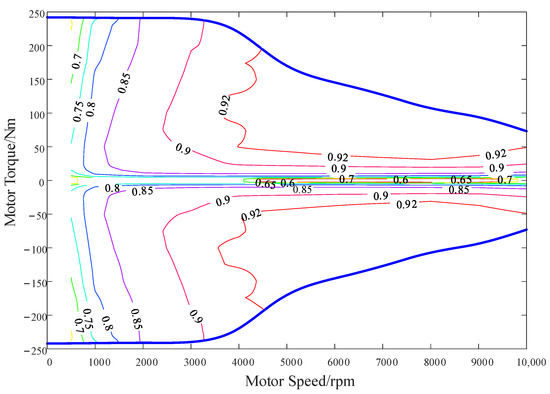
Figure 1. Efficiency map of the electrical machine.

2.3. Battery Model

Batteries are the energy source for electric vehicles. Accurately obtaining the SOC and SOH of the battery can lead to better performance, improve energy utilization, and extend the service life of the battery.

2.3.1. Energy Loss Model

An accurate battery model is conducive to better battery management which allows full use to be made of the battery’s performance. In accordance with the model mechanism, battery models can be divided into: electrochemical models, equivalent circuit models, neural network models and so on [34]. The model established according to the chemical reaction mechanism of the battery is called the electrochemical model, and this can accurately simulate the main characteristics of the battery. However, this model is complicated and has too many parameters, meaning it is difficult to calculate and is not suitable for control design [35]. The neural network model simulates the state change of the battery through the training and self-learning of the internal parameter data, but it requires a large volume of calculations and a long processing time [36]. The equivalent circuit model simplifies the reaction mechanism of the battery, reduces the number of calculations required for the model, and can reflect the battery mechanism. It is the current mainstream battery model [37].

In summary, to meet control requirements, an equivalent circuit model is adopted in this article. In references [11,38], the Rint model is used to account for the dynamic energy consumption of the batteries, and the verification results show that the model is accurate [4]. The Rint model has few parameters, which allows for faster controller calculations, as shown in Figure 2.

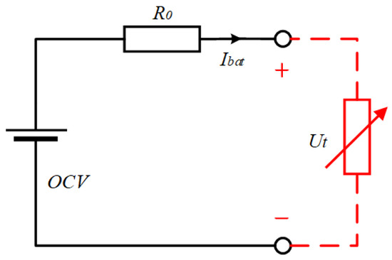
Figure 2. Rint circuit model.

According to the Rint circuit model, the output power and output voltage of the battery are expressed as Formula (3):

$$\left\{\begin{array}{l}{P}_{bat}=I_{bat}\cdot U_t\\ U_t=OCV-I_{bat}{R}_0\end{array}\right.$$

(3)

where P_bat is the power of the battery; I_bat is the output current of the battery; U_t is the output voltage of the battery; OCV is the open circuit voltage of the battery, which changes with the SOC of the battery; and R₀ is the ohmic resistance of the battery.

In this study, the Lishen 20 AH lithium iron phosphate battery produced by a company was selected as the experimental object, and some of its specific parameters are shown in Table 2. The experimental equipment was a 5 V–20 A range battery test cabinet from Ningbo Baite Measurement and Control Co., Ltd. (Ningbo, China), a LW-150 high- and low-temperature test box from Shanghai Haixiang Instrument and Equipment Co., Ltd. (Shanghai, China), and a host computer. The battery test system shown in Figure 3 consisted of a thermostat used to set the test environment temperature for the battery, an upper computer used to design the test conditions for the battery and record the charge and discharge data of the battery, and a battery testing box used to test the battery according to the set charging and discharging conditions.

Table 2. Battery parameters.

Parameters (Unit)	Value	Parameters (Unit)	Value
Rated voltage Vcell (V)	3.2	Charging voltage (V)	3.65 $\pm$ 0.05
Rated Capacity Qini (Ah)	20	Cut-off resistance R0,EOL ($\mathsf{\Omega }$)	0.0107
Initial resistance R0,new ($\mathsf{\Omega }$)	0.0063	Operating temperature (°C)	−20~45
Number of batteries in series	45	Number of parallel batteries	6

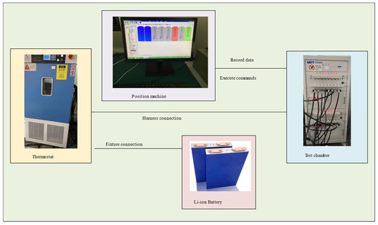
Figure 3. Battery test system.

The experimental results show that the OCV-SOC data of the battery can be fitted to a curve, as shown in Figure 4.

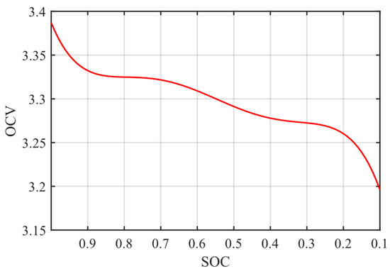
Figure 4. OCV-SOC curve.

The SOC of the battery is calculated by the ampere-hour method, which is expressed as Formula (4):

$$SOC=SO{C}_{ini}-\frac{1}{Q_{now}}{\displaystyle {\int }_0^t{\eta }_b{I}_{\mathrm{bat}}}dt$$

(4)

where SOC_ini is the initial value of the battery; Q_now is the current capacity of the battery; and η_b is the efficiency of the battery.

2.3.2. Battery Capacity Decay Model

At present, many scholars have found through experiments that a battery’s charge–discharge rate, temperature, and discharge depth are the main reasons for the battery’s capacity decline [39]. Therefore, this study uses a semi-empirical model based on experimental data to estimate the battery’s capacity decay. The evaluation index is expressed as Formula (5):

$$\left\{\begin{array}{l}{Q}_{loss}=A\cdot \exp (-\frac{E_a+B\cdot C_{rate}}{R\cdot T})\cdot {\mathrm{Ah}}^z\\ Ah=2\times N_{cyc}\times DOD\times Q_{cell}\end{array}\right.$$

(5)

where Q_loss is the battery capacity loss; A, B and z are the parameters to be fitted; E_a is the activation energy(J·mol⁻¹), take E_a = 31,700; R is the gas constant, take R = 8.314; T is the working ambient temperature of the battery in K; Ah is the accumulated current flow of the battery; DOD is the depth of discharge; and Q_cell is the capacity of the battery.

In this paper, we defined the SOH of the battery based on its capacity and, in accordance with the capacity decay of the battery, we obtained the current SOH and actual available capacity of the battery through Formula (6):

$$\left\{\begin{array}{l}\mathrm{SOH}=\frac{Q_{\mathrm{now}}-Q_{\mathrm{EOL}}}{Q_{\mathrm{new}}-Q_{\mathrm{EOL}}}\\ Q_{now}=(1-Q_{loss})\times Q_{ini}\end{array}\right.$$

(6)

Xia et al. [40] pointed out that there is a linear relationship between battery capacity decline and battery internal resistance, which is expressed as:

$$Q_{loss}=k\cdot R_{0,now}+b$$

(7)

where R_0,now is the ohmic resistance value of the current battery. Substituting Formula (7) into Formula (6), we can obtain:

$$\frac{Q_{\mathrm{now}}-Q_{\mathrm{EOL}}}{Q_{\mathrm{new}}-Q_{\mathrm{EOL}}}=\frac{Q_{\mathrm{loss},\mathrm{EOL}}-Q_{\mathrm{loss},\mathrm{now}}}{Q_{\mathrm{loss},\mathrm{EOL}}-Q_{\mathrm{loss},\mathrm{new}}}$$

(8)

where Q_EOL is the capacity of the battery to reach the EOL state; Q_new is the capacity of the new battery; and Q_now is the current capacity of the battery. Substituting Formula (7) into Formula (8), we can obtain:

$$\frac{Q_{now}-Q_{EOL}}{Q_{new}-Q_{EOL}}=\frac{R_{0,EOL}-R_{0,now}}{R_{0,EOL}-R_{0,new}}$$

(9)

where R_0,EOL is the resistance value of the battery at the end of life (EOL) and R_0,new is the internal resistance of the new battery. By transforming Formula (9), the internal resistance in the battery model is expressed as:

$$R_{0,now}=R_{0,EOL}-\frac{Q_{now}-Q_{EOL}}{Q_{new}-Q_{EOL}}(R_{0,EOL}-R_{0,new})$$

(10)

Based on the derivation analysis of the above formula, we obtained the relationship between battery capacity and internal resistance in the equivalent circuit model. Next, the lithium-ion battery was subjected to charging and discharging experiments under different test conditions to obtain the battery capacity degradation curve. As the number of charge and discharge cycles increased, the Ah passing through the battery also gradually increased. The relationship between the Ah passing through the battery and the battery capacity degradation rate is shown in Figure 5. The battery was tested at different DODs and ambient temperatures. The capacity measured at different temperatures was compensated by a compensation coefficient, and the battery capacity equivalent to 25 °C was obtained. Then, the experimental results were curve-fitted, and the fitting parameters were A = 53.86, B = −9.868, and z = 0.6749.

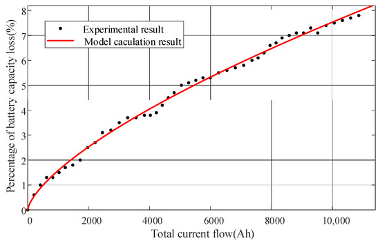
Figure 5. Battery capacity decay curve.

3. Adaptive Cruise Controller Design

3.1. MPC Controller Design

Based on the state between vehicles as shown in Figure 6, this study establishes a cost function that can reflect tracking comfort and economy, and which blurs the weight coefficient between the performances in accordance with different driving conditions to determine optimal acceleration.

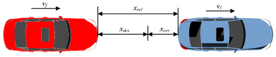
Figure 6. Vehicle-following scenario.

3.1.1. State Space Equation

In this study, the acceleration of the vehicle was used as the control quantity, and the state variables between vehicles in the following state were established. The relative distance and relative velocity were expressed as Formula (11):

$$\left\{\begin{array}{l}{x}_{\mathit{rel}}=x_l-x_f\\ v_{rel}=v_l-v_f\end{array}\right.$$

(11)

where x_rel is the relative distance between the two vehicles; x_l is the displacement of the leading vehicle; x_f is the displacement of the following vehicle; v_rel is the relative speed; v_l is the speed of the leading vehicle; and v_f is the speed of the following vehicle.

Considering the distance between the two vehicles and the relative speed, we defined the state variables X(k) and output Y(k) for the subsequent calculation of MPC:

$$\left\{\begin{array}{l}X(k)={[x_{rel}(k),v_{rel}(k),v_f(k),a(k),j(k)]}^T\\ Y(k)={[x_{rel}(k),v_{rel}(k),a(k),j(k)]}^T\\ Y(k)=DX(k)\end{array}\right.$$

(12)

where, a(k) is the acceleration of the host vehicle at time k; j(k) is the jerk of the host vehicle at time k; $and D=\left[\begin{array}{ccccc}1& 0& 0& 0& 0\\ 0& 1& 0& 0& 0\\ 0& 0& 0& 1& 0\\ 0& 0& 0& 0& 1\end{array}\right]$.

We set up a constant headway strategy to arrive at the desired distance:

$$x_{des}=v_f\cdot {\tau }_t+d_0$$

(13)

where x_des is the desired distance between vehicles; ${\tau }_t$ is the constant time interval; and d₀ is the minimum safe distance.

Due to the inertial and nonlinear nature of the vehicle’s drivetrain, there is a certain delay in the actual acceleration of the vehicle when following the desired acceleration. Therefore, a first-order inertial linkage was used in the design to represent the actual transmission characteristics [15], as shown in Formula (14):

$$a=\frac{1}{\tau s+1}{a}_{des}$$

(14)

where a_des is the desired acceleration and $\tau$ is the inertial link time constant.

Establishing a state space model between two vehicles and discretizing it, we arrived at:

$$\left\{\begin{array}{l}{x}_{rel}(k+1)=x_{rel}(k)+v_{rel}(k)\cdot ts\\ v_{rel}(k+1)=[a_l(k)-a_f(k)]\cdot ts+v_{rel}(k)\\ v(k+1)=v(k)+a(k)\cdot ts\\ a(k+1)=(1-\frac{ts}{\tau })a(k)+\frac{ts}{\tau }{a}_{des}(k)\\ j(k+1)=-\frac{1}{\tau }a(k)+\frac{1}{\tau }{a}_{des}(k)\end{array}\right.$$

(15)

Converting Formula (15) into matrix form, we arrived at: X(k + 1) = AX(k) + Bu(k) + Cal(k), which is expressed as Formula (16):

$$\left(\begin{array}{l}{x}_{rel}(k+1)\\ v_{rel}(k+1)\\ v(k+1)\\ a(k+1)\\ j(k+1)\end{array}\right)=\left(\begin{array}{ccccc}1& ts& 0& 0& 0\\ 0& 1& 0& -ts& 0\\ 0& 0& 1& ts& 0\\ 0& 0& 0& -\frac{ts}{\tau }& 0\\ 0& 0& 0& -\frac{1}{\tau }& 0\end{array}\right)\left(\begin{array}{l}{x}_{rel}(k)\\ v_{rel}(k)\\ v(k)\\ a(k)\\ j(k)\end{array}\right)+\left(\begin{array}{c}\begin{array}{l}0\\ 0\end{array}\\ 0\\ \frac{ts}{\tau }\\ \frac{1}{\tau }\end{array}\right)u(k)+\left(\begin{array}{c}\begin{array}{l}0\\ ts\end{array}\\ 0\\ 0\\ 0\end{array}\right)a_l(k)$$

(16)

where ts is the sampling time; u(k) is the control variable at time k; and a_l(k) is the disturbance at time k. This is the acceleration of the preceding vehicle.

Therefore, X_k under the prediction step N can be expressed as Formula (17):

$$X_k=M_{1}x(k)+M_2{U}_k+M_3{a}_{lk}$$

(17)

where $X_k=\left(\begin{array}{c}X(k)\\ X(k+1)\\ ⋮\\ \begin{array}{l}X(k+N-1)\\ X(k+N)\end{array}\end{array}\right)$; $U_k=\left(\begin{array}{c}U(k)\\ U(k+1)\\ ⋮\\ U(k+N-1)\end{array}\right)$; $a_{lk}=\left(\begin{array}{c}{a}_p(k)\\ a_p(k+1)\\ ⋮\\ a_p(k+N-1)\end{array}\right)$;

$$M_1=\left(\begin{array}{c}I\\ A\\ ⋮\\ \begin{array}{l}{A}^{N-1}\\ A^N\end{array}\end{array}\right);M_2=\left(\begin{array}{cccc}0& 0& \cdots & 0\\ B& 0& \cdots & 0\\ AB& B& \cdots & 0\\ ⋮& ⋮& \dots & ⋮\\ A^{N-1}B& A^{N-2}B& \cdots & B\end{array}\right);M_3=\left(\begin{array}{cccc}0& 0& \cdots & 0\\ C& 0& \cdots & 0\\ AC& C& \cdots & 0\\ ⋮& ⋮& \dots & ⋮\\ A^{N-1}C& A^{N-2}C& \cdots & C\end{array}\right)$$

According to Y(k) = DX(k), it can be concluded that Y_k under the prediction step N can be expressed as Formula (18):

$$Y_k=\left(\begin{array}{c}Y(k)\\ Y(k+1)\\ ⋮\\ \begin{array}{l}Y(k+N-1)\\ Y(k+N)\end{array}\end{array}\right)=L_1{X}_k+L_2{U}_k+L_3{a}_l{}_k$$

(18)

where $L_1=\left(\begin{array}{c}D\\ DA\\ ⋮\\ \begin{array}{l}D{A}^{N-1}\\ D{A}^N\end{array}\end{array}\right)$; $L_2=\left(\begin{array}{cccc}0& 0& \cdots & 0\\ DB& 0& \cdots & 0\\ DAB& DB& \cdots & 0\\ ⋮& ⋮& \dots & ⋮\\ D{A}^{N-1}B& D{A}^{N-2}B& \cdots & DB\end{array}\right)$; $L_3=\left(\begin{array}{cccc}0& 0& \cdots & 0\\ DC& 0& \cdots & 0\\ DAC& DC& \cdots & 0\\ ⋮& ⋮& \dots & ⋮\\ D{A}^{N-1}C& D{A}^{N-2}C& \cdots & DC\end{array}\right)$.

3.1.2. Definition of Cost Function

Personnel safety is the most important part of the driving process of the vehicle. The main vehicle and the vehicle in front should always maintain a safe distance, that is, it must be ensured that x_rel > d₀ is always established.

The tracking performance is mainly reflected in the relative distance and relative speed of the two vehicles while driving. In order to improve the tracking performance of the vehicle while driving, the cost function of tracking performance was defined:

$$J_{tracking}={\displaystyle \sum _{i=1}^N[{\left(x_{rel}(k+i)-x_{ref}(k+i)\right)}^2+{\left(v_{rel}(k+i)-v_{ref}(k+i)\right)}^2]}$$

(19)

Comfort is mainly a reflection of the impact on passengers when the vehicle accelerates or brakes. In order to improve the riding comfort of passengers, the cost function of comfort was defined and constraints were set with the goal of reducing acceleration and jerk during driving:

$$\begin{array}{c}{J}_{comfort}={\displaystyle \sum _{i=1}^N[a^2(k+i)+j^2(k+i)]}\\ \left\{\begin{array}{l}{a}_{\min }<a(k)<a_{\max }\\ j_{\min }<j(k)<j_{\max }\end{array}\right.\end{array}$$

(20)

The decay characteristic of the battery is reflected in the reduction in available capacity. The Q_loss described above can objectively evaluate the decay of the battery, and define the cost function:

$$J_{loss}={\displaystyle \sum _{i=1}^N{Q}_{loss}(i)}$$

(21)

Combining the above cost functions, the cost function of the entire control process was obtained:

$$J={\omega }_1\cdot J_{tracking}+{\omega }_2\cdot J_{comfort}+{\omega }_3\cdot J_{loss}$$

(22)

where ω₁, ω₂, ω₃ represent the weights of tracking, comfort, and battery capacity degradation characteristics, respectively.

In order to improve computational efficiency, we simplified the cost function. First of all, we took J₁ = ω₁$·$J_tracking + ω₂$·$J_comfort, and arrived at J₁$={\displaystyle \sum }_{i=1}^N{\left[Y\left(k+i\right)-Y_{ref}\left(k+i\right)\right]}^{\mathrm{T}}Q\left[Y\left(k+i\right)-Y_{ref}\left(k+i\right)\right]$, so J₁ = (Y_k − Y_ref)^TQ(Y_k − Y_ref), where Q is the weight matrix. Y_ref = [x_des, 0, 0, 0]^T indicates that the expected value of the relative distance is the expected distance and the relative speed, and the absolute value of the acceleration of the main vehicle and the shock degree during the driving process are at their smallest. We took L₁$·$x(k) + L3$·$a_lk = E and combined Formula (18) to arrive at Y_k − Y_ref = E + L₂$·$U_k − Y_ref, so J₁ can be transformed into Formula (23):

$$\begin{array}{l}{J}_1=(E+L_2{U}_k-Y_{ref}{)}^{T}Q(E+L_2{U}_k-Y_{ref})=E^{T}QE+2E^{T}Q{L}_2{U}_k\\ \hspace{1em}\hspace{1em}-2E^{T}Q{Y}_{ref}-2Y_{ref}{}^{T}Q{L}_2{U}_k+U_k{}^T{L}_2{}^{T}Q{L}_2{U}_k+Y_{ref}{}^{T}Q{Y}_{ref}\end{array}$$

(23)

By eliminating polynomials that have no effect on the control outcome, a new cost function J₁^* for integrated tracking and comfort can be obtained, as shown in Formula (24):

$$J_1^{*}=2(E^{T}Q{L}_2-Y_{ref}{}^{T}Q{L}_2)U_k+U_k{}^T{L}_2{}^{T}Q{L}_2{U}_k$$

(24)

When setting weights in traditional MPC controllers, the cost function is often designed with fixed weights which cannot consider the performance requirements of the vehicle under different driving conditions. Therefore, this study designed a variable weight cost function.

3.1.3. Design of Fuzzy Weight

As an intelligent algorithm, fuzzy control is robust and can provide solutions for nonlinear time-varying systems and systems that are difficult to model. In addition, since the fuzzy rules can be changed at any time, it has good adaptability to the system [41]. Therefore, this study used a fuzzy control algorithm to optimize the weights. Taking the distance error (the difference between the actual distance and the expected distance) and the main vehicle speed as input, and taking the economic weight as the output, the main vehicle speed domain was set to [0, 140] m/s and the relative distance domain was set to [−5, 5] m. The main vehicle speed was divided into three types according to speed value, and the corresponding logical language was {S, M, B}. The distance error was divided into 7 types according to error value, and the corresponding logical language was {NB, NM, NS, Z, PS, PM, PB}. To fuzzy the economic weights, the logical language was {S, MS, M, MB, B}, and the range of variation was [0, 20]. Both the input variables d_err and v_f, and the output variable ω_3, used trigonometric membership functions, as shown in Figure 7. Through the analysis of traffic scenarios, it was found that when the speed is low, attention should be paid to following the driving to ensure safety, and the weight given to economic factors should be small. When the speed is high, the demand for tracking is reduced due to the long distance between vehicles, the focus is on economical driving, and the weight given to economy should be increased. The specific fuzzy rules are shown in Table 3. Since the barycenter method is intuitive, reasonable, simple, and accurate in control, the barycenter method was selected to deblur. The corresponding input and output results were obtained in accordance with the fuzzy rules, and the economic weight coefficient surface solved is shown in Figure 8.

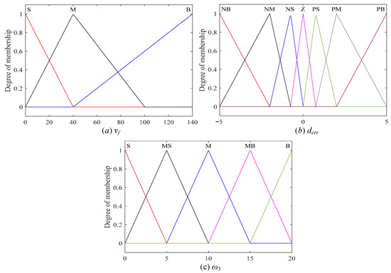
Figure 7. Membership function: (a) v_f, (b) d_err, (c) ω₃.

Table 3. Fuzzy rules design.

Economic Weight ω3 [0, 20]		derr = drel − ddes
		NB	NM	NS	Z	PS	PM	PB
vf	S [0, 40] M [40, 100] B [100, 140]	S	S	MS	MS	M	M	MS
		S	MB	MS	MB	B	M	MS
		MS	M	MB	B	B	MB	MS

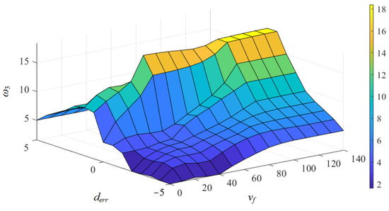
Figure 8. Relationship between distance error, v_f and the economic weight coefficient.

3.1.4. Solving Optimization Problems

Based on Formulas (22) and (24), the optimization problem that MPC needs to solve each time is shown in Formula (25):

$$\begin{array}{c}\underset{U_k}{\min }(J_1^{*}+J_{loss})\\ s.t.\left\{\begin{array}{l}{x}_{rel}(k)>d_0\\ SO{C}_{\min }<SOC(k)<SO{C}_{\max }\\ a_{\min }<a<a_{\max }\\ j_{\min }<j<j_{\max }\end{array}\right.\end{array}$$

(25)

4. Performance Analysis

Based on the MATLAB platform, the acceleration curve of the electric vehicles was optimized by using the AMPC algorithm, and was compared with PID, SMC, MPC1 and MPC2 controllers, where the MPC1 controller does not consider the battery degradation characteristics, and the MPC2 controller considers the battery degradation characteristics and designs the cost function with fixed weights. The preset parameters of the controller are shown in Table 4 and Table 5, and the ambient temperature for battery operation was set to maintain 25 degrees Celsius.

Table 4. Parameters in PID, SMC, MPC1 controllers.

Parameters (Unit)	Value	Parameters (Unit)	Value
Prediction horizon N	20	Time headway (s)	1.5
Sampling time ts (s)	0.05	Minimum safe distance d0 (m)	4
Minimum acceleration (m/s2)	−5	Maximum acceleration (m/s2)	3
Minimum jerk (m/s3)	−2.5	Maximum jerk (m/s3)	2.5
Tracking weight parameter $\mathsf{\omega }$1	1	Comfort weight parameter $\mathsf{\omega }$2	0.1

Table 5. Economic weight parameters of MPC2.

Parameters (Unit)	Condition	Value
Economic weight parameter $\mathsf{\omega }$3	𝑣 < 40 km/h	5
	𝑣 ≥ 40 km/h	10

4.1. Safety and Comfort Analysis

The simulation conditions were set to the WLTC (Worldwide Harmonized Light Duty Test Cycle), which includes a series of operations such as acceleration, deceleration, constant speed driving, emergency braking, etc., to simulate the real driving conditions in the city. This working condition does not consider the impact of road slope, and the total cycle time is 1800 s. When driving under WLTC conditions, the minimum inter-vehicle distance under the action of each controller is shown in Table 6.

Table 6. Minimum distance between two vehicles under the action of each controller.

Controller	Minimum Inter-Vehicle Distance (m)
PID	5.0000
SMC	5.0333
MPC1	5.0021
MPC2	4.8735
AMPC	4.8679

The minimum distance between two vehicles usually occurs when the preceding vehicle brakes to speed 0, and the host vehicle slows down in the process. It can be seen from Table 6 that each controller can meet the preset safety distance, thus ensuring the safety of the driving process. The PID controller has the best followability; however, superior followability is accompanied by a drastic change in torque, and this will reduce energy utilization and lead to a decline in battery life.

At the initial moment, the vehicle in front was set to 8 m away from the host vehicle. Figure 9 shows the acceleration and impact of the vehicle under the action of each controller under the WLTC driving conditions. We defined passenger comfort as being guaranteed when the jerk is kept at (−2.5, 2.5). From Figure 9, it can be seen that, apart from the SMC controller which is out of range at the beginning of the simulation phase, the controllers meet the comfort requirements.

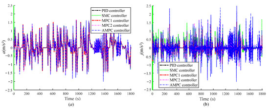
Figure 9. The acceleration and jerk of the host vehicle under each controller, (a) acceleration,(b) jerk.

4.2. Tracking and Economic Analysis

In the initial phase of the simulation, the vehicle was set 8 m in front of the host vehicle, and the SOH of the battery was set to 1. Figure 10 shows a comparison between the expected and actual distances between the two vehicles with the PID, SMC, MPC1, MPC2, and AMPC controllers, respectively. It can be found that under the PID, SMC and MPC1 controllers, both vehicles show better tracking ability. Excellent tracking performance is accompanied by frequent changes in electric machine torque and battery current, resulting in increased energy consumption and shorter service life. Therefore, for this paper, we designed economic indicators and variable weight coefficients to ensure low-speed tracking while considering the economy of high-speed following. As shown in Figure 10, a controller that takes the aging characteristics of the battery into account will exceed the expected distance during the high-speed driving phase. However, when the vehicle is driving at a high speed, the larger following distance can ensure that when the car in front brakes suddenly, the main car has enough distance to brake, ensuring safety. Figure 11 shows the tracking speed curves with the PID, SMC, MPC1, MPC2 and AMPC controllers. As can be seen from Figure 11, in the low-speed section, due to the small economic weight, the effect of each controller is similar. In the medium-speed section, due to the increase in speed, the economic weight is gradually increased and the MPC2 and AMPC controllers, which consider the aging characteristics of the battery, are slower than the other controllers. This reduces the output of electric machine torque while ensuring acceleration and following driving, which is conducive to improving driving economy. In the high-speed segment, the AMPC controller is more effective.

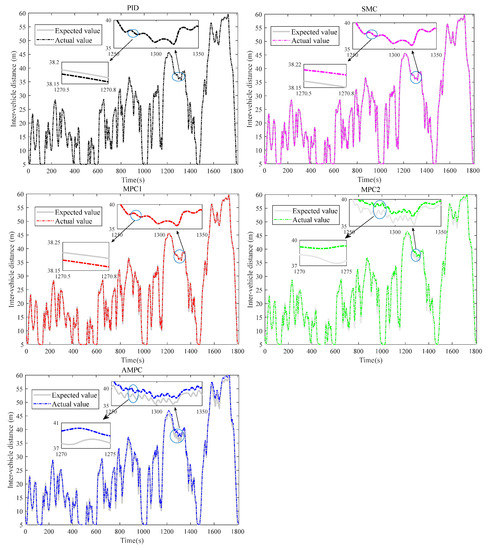
Figure 10. Distance tracking curve of each controller.

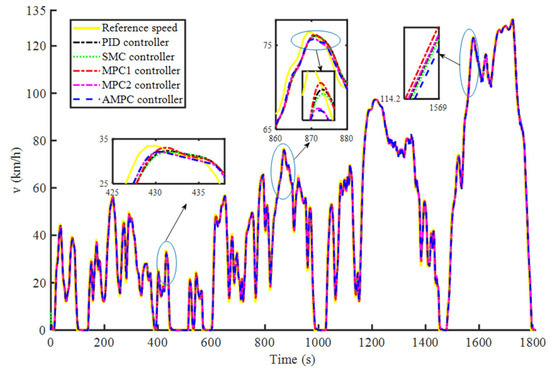
Figure 11. Speed tracking curve of each controller.

Figure 12 shows the current curve of the battery cells when the main vehicle was driving under the action of each controller. At low speeds, the current of the battery under the action of the MPC2 and AMPC controllers was smaller than under the rest of the controllers. In the medium- and high-speed section, it can be seen from the current curve that the vehicle will adopt an acceleration-coasting method to reduce the continuous output of battery current during driving and to improve driving economy.

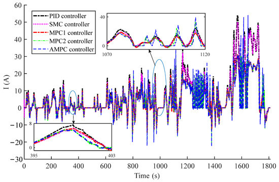
Figure 12. Current curve of each controller.

Figure 13a shows the capacity attenuation curve of the battery under each control, and Figure 13b shows the SOC decline curve, the specific value of which is shown in Table 7.

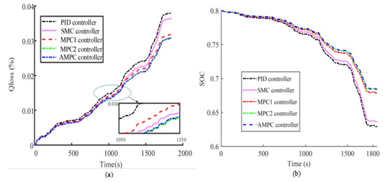
Figure 13. Under WLTC working conditions, the battery (SOHini = 1) parameters under the action of each controller: (a) battery capacity loss (b) SOC.

Table 7. Capacity loss value and SOC of battery under each controller after the WLTC (SOHini = 1).

Controller	PID	SMC	MPC1	MPC2	AMPC
Qloss (‱)	3.8063	3.6463	3.1877	3.0822	3.0835
SOC	0.6295	0.6364	0.6789	0.6841	0.6846

Since the MPC controller can optimize multiple targets during driving, that is it can limit the acceleration and jerk of the host vehicle, it can be seen from Table 6 that the decline rate of battery capacity under the MPC controller is better mitigated compared to under the PID and SMC controllers. Compared to the MPC1, MPC2 and AMPC controllers, controllers that consider battery degradation characteristics further reduce battery capacity degradation. Compared with the PID, SMC, MPC1 and MPC2 controllers, the battery capacity attenuation was reduced by 18.99%, 15.43%, 3.27% and −0.04%, respectively, and the battery energy consumption was reduced by 32.32%, 29.46%, 4.71% and 0.43%, respectively, indicating that under the condition of battery SOH = 1, the AMPC controller can more effectively improve the energy utilization of the battery, while the MPC2 controller will improve the service life more effectively. This shows that the control method that optimizes energy consumption is not necessarily optimal for life improvement.

In order to further verify that the battery attenuation characteristic controller proposed in this study is still effective after battery degradation, the battery SOH was set to 0.9 for verification. Figure 14 shows the battery capacity attenuation curve and the SOC degradation curve for each controller, as shown in Table 8.

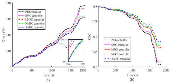
Figure 14. Under WLTC working conditions, the battery (SOHini = 0.9) parameters under the action of each controller: (a) battery capacity loss (b) SOC.

Table 8. Capacity loss value and SOC of battery under each controller after the WLTC (SOHini = 0.9).

Controller	PID	SMC	MPC1	MPC2	AMPC
Qloss (‱)	3.8390	3.6642	3.2015	3.0984	3.0967
SOC	0.6295	0.6157	0.6643	0.6700	0.6846

As the battery’s state of health decreases, the resistance in the battery model increases, the battery current demand increases significantly when the vehicle is driving at high speeds, and the AMPC controller is more effective in reducing energy consumption and extending service life.

In order to verify the adaptability of the method to working conditions, the performance of the battery controller under different SOH conditions, different working conditions and different cycle times of working conditions was compared. Figure 15 shows the battery capacity degradation curve and the SOC reduction curve under the action of each controller when the vehicle is driving under 5 WLTCs. It can be seen that the controller which takes battery aging characteristics into account performs better, and after the simulation, the battery still has a certain amount of power, while the PID and SMC controllers ran out of power during the simulation. In Table 7, it can be seen that when the battery SOH = 1, the MPC2 controller performs better than the AMPC controller in extending battery life, and with the increase in simulation time, the high-speed driving time also increases. Within this range, the increase in the economic weight in the cost function of the AMPC controller can make economic adjustments to the driving state, as shown in Figure 15a. In the simulation process, when driving in the high-speed range, the effect of the AMPC controller on life optimization was better than that of the MPC2 controller. This slows down the rise rate of Q_loss.

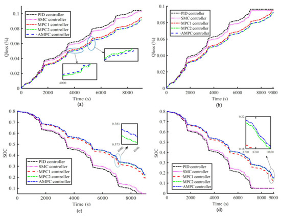
Figure 15. Under 5 WLTCs, the battery parameters under the action of each controller: when SOH = 1, (a) battery capacity loss (c) SOC. When SOH = 0.9, (b) battery capacity loss (d) SOC.

Next, the UDDS working conditions were simulated and verified, and Figure 16 shows the Qloss and SOC changes in the battery under different SOH conditions. Figure 16a shows that, under the action of the AMPC controller, the vehicle driving adopts the acceleration-coasting method, which can slow down the capacity decline process of the battery. Figure 16b shows the change in battery SOC, and it can be seen that the controller which considers the aging characteristics of the battery can effectively reduce energy consumption. The specific values are shown in Table 9.

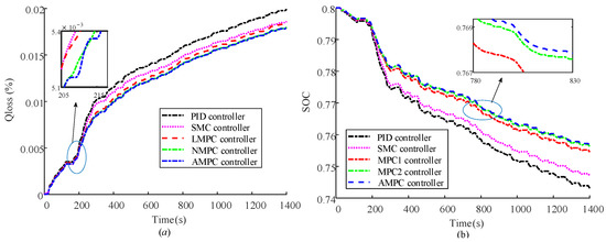
Figure 16. Under UDDS working conditions, the battery (SOHini = 1) parameters under the action of each controller: (a) battery capacity loss (b) SOC.

Table 9. Capacity loss value and the SOC of the battery under each controller after UDDS cycle (SOHini = 1).

Controller	PID	SMC	MPC1	MPC2	AMPC
Qloss (‱)	1.9921	1.8604	1.8418	1.7978	1.7940
SOC	0.7431	0.7470	0.7545	0.7562	0.7566

Figure 17 shows the battery capacity degradation curve and SOC reduction curve when the vehicle is driving under 10 UDDS cycles, showing that the AMPC controller performs better in terms of energy savings and life optimization.

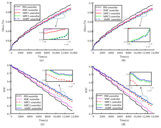
Figure 17. Under 10 UDDS cycles, the battery parameters under the action of each controller: when SOH = 1, (a) battery capacity loss (c) SOC. When SOH = 0.9, (b) battery capacity loss (d) SOC.

Finally, the NEDC working conditions were simulated and compared. The battery parameter changes are shown in Figure 18. Figure 18a shows that under the NEDC working conditions, the MPC2 controller has advantages in life optimization and energy consumption as most of the NEDC working conditions are medium- and low-speed conditions, and the economic coefficient of the fixed weight controller is higher than the variable weight coefficient, which can effectively improve the battery energy utilization rate after ensuring the safety and comfort of driving. Moreover, controllers that consider the decay of battery capacity have significantly improved energy consumption and life optimization compared to other controllers, and the specific values are shown in Table 10.

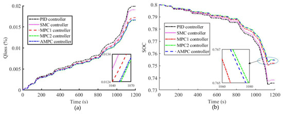
Figure 18. Under NEDC working conditions, the battery (SOHini = 1) parameters under the action of each controller: (a) battery capacity loss (b) SOC.

Table 10. Capacity loss value and SOC of the battery under each controller after the NEDC (SOHini = 1).

Controller	PID	SMC	MPC1	MPC2	AMPC
Qloss(‱)	1.9921	1.8604	1.8418	1.7978	1.7940
SOC	0.7431	0.7470	0.7545	0.7562	0.7566

Figure 19 shows the battery capacity degradation curve and the SOC degradation curve when the vehicle is driven under 10 NEDCs. The MPC2 controller outperforms the AMPC controller with the same results as a single NEDC, which can effectively mitigate the degradation of battery capacity.

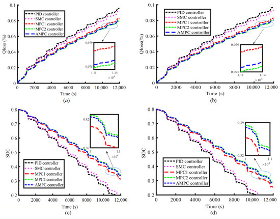
Figure 19. Under 10 NEDCs, the battery parameters under the action of each controller: when SOH = 1, (a) battery capacity loss (c) SOC. When SOH = 0.9, (b) battery capacity loss (d) SOC.

Based on the above result analysis, when the vehicle is driving under high-speed complex working conditions, such as WLTC working conditions, and with a new battery (SOH = 1), when optimizing the battery life is the goal, the fixed weight controller MPC2 is more effective. When the battery declines, the variable weight controller AMPC performs better. When the vehicle is driven in medium or low speed conditions, such as NEDC and UDDS standard working conditions, the fixed weight controller MPC2 performs better.

4.3. HIL Test Implementation

In order to ensure the effectiveness of the proposed strategy, hardware-in-the-loop testing was conducted in addition to software simulation. The HIL platform constructed in this study included ECU rapid prototyping based on D2P and a NI real-time simulation cabinet, as shown in Figure 20. The rapid prototyping based on MotoHawk included the modeling and code generation of the controller, and code flashing and debugging based on MotoTune. Information interaction was achieved through CAN communication with the NI real-time simulation cabinet. The hardware contained in the NI real-time simulation cabinet included a PXI chassis PXIe-1065, a real-time controller PXIe-8135, a digital input/output board PXI 7811R, an analog input board PXI-6224, an analog output board PXI-6224, two CAN bus board cards, and a fault injection board PXI 2510. The single WLTC was designed as the test condition, and the battery’s (SOH) was set to 1. The simulation results of the HIL are shown in Figure 21 and Figure 22. As shown in Figure 21, the vehicle speed obtained in HIL was roughly the same as the speed used for model validation. However, there were overshoot and lag phenomena at certain times, indicating that the response speed of the controller and the communication on the CAN bus had some impact on the proposed algorithm. The battery capacity degradation values for model-in-the-loop and hardware-in-the-loop testing are shown in Figure 22. Compared with the results of model-in-the-loop testing, the Qloss of hardware-in-the-loop testing is 0.688‰ higher. Overall, from the vehicle speed tracking and Qloss reduction curves, it can be seen that the proposed control algorithm has good real-time performance and can meet the requirements of the system.

Figure 20. Schematic diagram of HIL test platform.

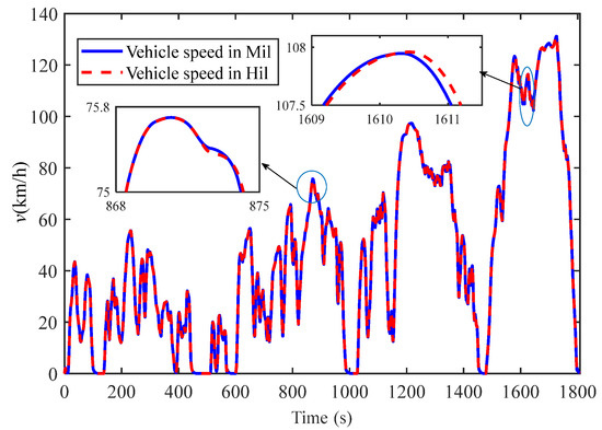
Figure 21. Speed comparison between simulation and Hil.

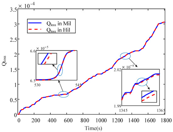
Figure 22. Q_loss compariso between simulation and Hil.

5. Conclusions

In this paper, a control method that considers the decay characteristics of battery capacity during tracking is proposed, aiming to extend the service life of the battery. First a model that can simulate the dynamics of the vehicle system was built, and then performance indicators that can characterize the driving state, such as comfort, tracking, and economy, were designed. The capacity decay model of the battery was established through experimental data, and the battery model was updated accordingly. Then the MPC controller was designed, the cost function was composed by weights and performance indicators, and the weight was designed by fuzzy control. Finally, the performance of the control method proposed in this study and the traditional controller at different battery SOH, different working conditions and different cycle times was verified by simulation. After the results were analyzed, it was seen that the follow-up control method which is proposed in this paper, and which considers the aging characteristics of the battery, can effectively optimize battery service life compared with traditional control methods. The proposed method was validated through hardware-in-the-loop testing and can meet the real-time requirements of the system. In future work, real road condition information will be collected to increase road realism, and controller switching logic will be added to achieve optimal control under different working conditions.

References

- Shahabi, A.; Kazemian, A.H.; Farahat, S.; Sarhaddi, F. The influence of engine gyroscopic moments on vehicle transient handling. Proc. Inst. Mech. Eng. Part D J. Automob. Eng. 2021, 235, 2425–2441. [Google Scholar] [CrossRef]
- Wang, G.; Wu, J.; Ma, X. A guaranteed cost strategy for speed-limit control of vehicles based on map information. Proc. Inst. Mech. Eng. Part D J. Automob. Eng. 2021, 235, 3127–3137. [Google Scholar] [CrossRef]
- Ma, F.; Yang, Y.; Wang, J.; Liu, Z.; Li, J.; Nie, J.; Shen, Y.; Wu, L. Predictive energy-saving optimization based on nonlinear model predictive control for cooperative connected vehicles platoon with V2V communication. Energy 2019, 189, 116120. [Google Scholar] [CrossRef]
- Chen, X.; Yang, J.; Zhai, C.; Lou, J.; Yan, C. Economic Adaptive Cruise Control for Electric Vehicles Based on ADHDP in a Car-Following Scenario. IEEE Access 2021, 9, 74949–74958. [Google Scholar] [CrossRef]
- Ren, Y.; Zheng, L.; Yang, W.; Li, Y. Potential field–based hierarchical adaptive cruise control for semi-autonomous electric vehicle. Proc. Inst. Mech. Eng. Part D J. Automob. Eng. 2018, 233, 2479–2491. [Google Scholar] [CrossRef]
- Li, L.; Liu, Q. Acceleration curve optimization for electric vehicle based on energy consumption and battery life. Energy 2019, 169, 1039–1053. [Google Scholar] [CrossRef]
- Lee, M.H.; Park, H.G.; Lee, S.H.; Yoon, K.S.; Lee, K.S. An adaptive cruise control system for autonomous vehicles. Int. J. Precis. Eng. Manuf. 2013, 14, 373–380. [Google Scholar] [CrossRef]
- Prabhakar, G.; Selvaperumal, S.; Nedumal Pugazhenthi, P. Fuzzy PD Plus I Control-based Adaptive Cruise Control System in Simulation and Real-time Environment. IETE J. Res. 2018, 65, 69–79. [Google Scholar] [CrossRef]
- Ganji, B.; Kouzani, A.Z.; Khoo, S.Y.; Shams-Zahraei, M. Adaptive cruise control of a HEV using sliding mode control. Expert Syst. Appl. 2014, 41, 607–615. [Google Scholar] [CrossRef]
- Gao, F.; Hu, X.; Li, S.E.; Li, K.; Sun, Q. Distributed adaptive sliding mode control of vehicular platoon with uncertain interaction topology. IEEE Trans. Ind. Electron. 2018, 65, 6352–6361. [Google Scholar] [CrossRef]
- Guo, J.; Li, W.; Wang, J.; Luo, Y.; Li, K. Safe and Energy-Efficient Car-Following Control Strategy for Intelligent Electric Vehicles Considering Regenerative Braking. IEEE Trans. Intell. Transp. Syst. 2021, 23, 7070–7081. [Google Scholar] [CrossRef]
- Wu, D.; Zhu, B.; Tan, D.; Zhang, N.; Gu, J. Multi-objective optimization strategy of adaptive cruise control considering regenerative energy. Proc. Inst. Mech. Eng. Part D J. Automob. Eng. 2019, 233, 3630–3645. [Google Scholar] [CrossRef]
- Wang, F.-X.; Peng, Q.; Zang, X.-L.; Xue, Q.-F. Adaptive Cruise Control for Intelligent City Bus Based on Vehicle Mass and Road Slope Estimation. Appl. Sci. 2021, 11, 12137. [Google Scholar] [CrossRef]
- Jia, Y.; Jibrin, R.; Gorges, D. Energy-Optimal Adaptive Cruise Control for Electric Vehicles Based on Linear and Nonlinear Model Predictive Control. IEEE Trans. Veh. Technol. 2020, 69, 14173–14187. [Google Scholar] [CrossRef]
- Pan, C.; Huang, A.; Wang, J.; Chen, L.; Liang, J.; Zhou, W.; Wang, L.; Yang, J. Energy-optimal adaptive cruise control strategy for electric vehicles based on model predictive control. Energy 2022, 241, 122793. [Google Scholar] [CrossRef]
- Samani, B.; Shamekhi, A.H. Multi-objective adaptive cruise controller design using nonlinear predictive controller with the objective function with variable weights determined by fuzzy logic controller. Proc. Inst. Mech. Eng. Part D J. Automob. Eng. 2021, 236, 142–154. [Google Scholar] [CrossRef]
- Shi, M.; He, H.; Li, J.; Han, M.; Jia, C. Multi-objective tradeoff optimization of predictive adaptive cruising control for autonomous electric buses: A cyber-physical-energy system approach. Appl. Energy 2021, 300, 117385. [Google Scholar] [CrossRef]
- He, Z.; Shen, X.; Sun, Y.; Zhao, S.; Fan, B.; Pan, C. State-of-health estimation based on real data of electric vehicles concerning user behavior. J. Energy Storage 2021, 41, 102867. [Google Scholar] [CrossRef]
- Christensen, J.; Newman, J. A Mathematical Model of Stress Generation and Fracture in Lithium Manganese Oxide. J. Electrochem. Soc. 2006, 153, A1019. [Google Scholar] [CrossRef]
- Shao, J.; Lin, C.; Yan, T.; Qi, C.; Hu, Y. Safety Characteristics of Lithium-Ion Batteries under Dynamic Impact Conditions. Energies 2022, 15, 9148. [Google Scholar] [CrossRef]
- Zhou, W. Effects of external mechanical loading on stress generation during lithiation in Li-ion battery electrodes. Electrochim. Acta 2015, 185, 28–33. [Google Scholar] [CrossRef]
- Ji, H.; Zhang, W.; Pan, X.H.; Hua, M.; Chung, Y.H.; Shu, C.M.; Zhang, L.J. State of health prediction model based on internal resistance. Int. J. Energy Res. 2020, 44, 6502–6510. [Google Scholar] [CrossRef]
- Zhou, W.; Hao, F.; Fang, D. The Effects of Elastic Stiffening on the Evolution of the Stress Field within a Spherical Electrode Particle of Lithium-Ion Batteries. Int. J. Appl. Mech. 2013, 5, 13500403. [Google Scholar] [CrossRef]
- Wang, J.; Liu, P.; Hicks-Garner, J.; Sherman, E.; Soukiazian, S.; Verbrugge, M.; Tataria, H.; Musser, J.; Finamore, P. Cycle-life model for graphite-LiFePO4 cells. J. Power Sources 2011, 196, 3942–3948. [Google Scholar] [CrossRef]
- Tang, L.; Rizzoni, G.; Onori, S. Energy Management Strategy for HEVs Including Battery Life Optimization. IEEE Trans. Transp. Electrif. 2015, 1, 211–222. [Google Scholar] [CrossRef]
- Zhuang, W.; Qu, L.; Xu, S.; Li, B.; Chen, N.; Yin, G. Integrated energy-oriented cruising control of electric vehicle on highway with varying slopes considering battery aging. Sci. China Technol. Sci. 2019, 63, 155–165. [Google Scholar] [CrossRef]
- Sun, X.; Liu, W.; Wen, M.; Wu, Y.; Li, H.; Huang, J.; Hu, C.; Huang, Z. A Real-Time Optimal Car-Following Power Management Strategy for Hybrid Electric Vehicles with ACC Systems. Energies 2021, 14, 3438. [Google Scholar] [CrossRef]
- Wu, J.; Wang, X.; Li, L.; Qin, C.a.; Du, Y. Hierarchical control strategy with battery aging consideration for hybrid electric vehicle regenerative braking control. Energy 2018, 145, 301–312. [Google Scholar] [CrossRef]
- Nie, Z.; Jia, Y.; Wang, W.; Chen, Z.; Outbib, R. Co-optimization of speed planning and energy management for intelligent fuel cell hybrid vehicle considering complex traffic conditions. Energy 2022, 247, 123476. [Google Scholar] [CrossRef]
- Vajedi, M.; Azad, N.L. Ecological Adaptive Cruise Controller for Plug-In Hybrid Electric Vehicles Using Nonlinear Model Predictive Control. IEEE Trans. Intell. Transp. Syst. 2016, 17, 113–122. [Google Scholar] [CrossRef]
- Brunner, J.S.; Makridis, M.A.; Kouvelas, A. Comparing the Observable Response Times of ACC and CACC Systems. IEEE Trans. Intell. Transp. Syst. 2022, 23, 19299–19308. [Google Scholar] [CrossRef]
- Al-Saadi, Z.; Phan Van, D.; Moradi Amani, A.; Fayyazi, M.; Sadat Sajjadi, S.; Ba Pham, D.; Jazar, R.; Khayyam, H. Intelligent Driver Assistance and Energy Management Systems of Hybrid Electric Autonomous Vehicles. Sustainability 2022, 14, 9378. [Google Scholar] [CrossRef]
- Althoff, M.; Maierhofer, S.; Pek, C. Provably-Correct and Comfortable Adaptive Cruise Control. IEEE Trans. Intell. Veh. 2021, 6, 159–174. [Google Scholar] [CrossRef]
- Wang, J.; Deng, Z. Modeling and predicting fecal coliform bacteria levels in oyster harvest waters along Louisiana Gulf coast. Ecol. Indic. 2019, 101, 212–220. [Google Scholar] [CrossRef]
- Pan, C. Lithium-ion Battery Remaining Useful Life Prediction Based on Exponential Smoothing and Particle Filter. Int. J. Electrochem. Sci. 2019, 14, 9537–9551. [Google Scholar] [CrossRef]
- Zhang, W.; Wang, L.; Wang, L.; Liao, C. An improved adaptive estimator for state-of-charge estimation of lithium-ion batteries. J. Power Sources 2018, 402, 422–433. [Google Scholar] [CrossRef]
- Zhao, W.; Kong, X.; Wang, C. Combined estimation of the state of charge of a lithium battery based on a back-propagation– adaptive Kalman filter algorithm. Proc. Inst. Mech. Eng. Part D J. Automob. Eng. 2017, 232, 357–366. [Google Scholar] [CrossRef]
- Sun, X.; Jin, Z.; Xue, M.; Tian, X. Adaptive ECMS with Gear Shift Control by Grey Wolf Optimization Algorithm and Neural Network for Plug-in Hybrid Electric Buses. IEEE Trans. Ind. Electron. 2023, 2023, 3243304. [Google Scholar] [CrossRef]
- Zou, Y.; Hu, X.; Ma, H.; Li, S.E. Combined State of Charge and State of Health estimation over lithium-ion battery cell cycle lifespan for electric vehicles. J. Power Sources 2015, 273, 793–803. [Google Scholar] [CrossRef]
- Xia, Z.; Qahouq, J.A.A.; Phillips, E.; Gentry, R. A simple and upgradable autonomous battery aging evaluation and test system with capacity fading and AC impedance spectroscopy measurement. In Proceedings of the 2017 IEEE Applied Power Electronics Conference and Exposition (APEC), Tampa, FL, USA, 26–30 March 2017; pp. 951–958. [Google Scholar]
- Phu, N.D.; Hung, N.N.; Ahmadian, A.; Senu, N. A New Fuzzy PID Control System Based on Fuzzy PID Controller and Fuzzy Control Process. Int. J. Fuzzy Syst. 2020, 22, 2163–2187. [Google Scholar] [CrossRef]
Disclaimer/Publisher’s Note: The statements, opinions and data contained in all publications are solely those of the individual author(s) and contributor(s) and not of MDPI and/or the editor(s). MDPI and/or the editor(s) disclaim responsibility for any injury to people or property resulting from any ideas, methods, instructions or products referred to in the content. |
© 2023 by the authors. Licensee MDPI, Basel, Switzerland. This article is an open access article distributed under the terms and conditions of the Creative Commons Attribution (CC BY) license (https://creativecommons.org/licenses/by/4.0/).