Main Factors on Effect of Precise Measurement and Precise Tamping Based on BP Neural Network

Abstract

With the continuous development of precise measurement and precise tamping (PMPT) technology on Chinese railway conventional speed lines, the efficiency of machinery tamping operation and the quality of the track have been effectively improved. A variety of PMPT modes have been tried in the field operation, however there are some differences in the operation effect. The quality of the tamping operation is affected by multiple factors. In order to identify the key factors affecting the operation quality and to further improve the tamping operation effect, this paper establishes both the database of PMPT operation modes and the selection index system for evaluating the operation effect. Based on mega multi-source heterogeneous data and track geometry inspection data, this paper adopts the Back Propagation Neural Network (BPNN) prognosis model to quantify and sort the main factors affecting the effect of PMPT. The research results show that the initial quality of the track before tamping, whether the stabilizing operation or the tamping modes have great influence weights. It can scientifically guide the field operation to control the key factors and put forward some practical suggestions for promoting the field application of PMPT and the optimization of operation modes on the conventional speed lines.

1. Introduction

The application of heavy-duty track maintenance machinery to realize digitally-controlled tamping operation and repairing the tracks by sections is an effective means to eliminate the ballasted track irregularities at the longitudinal level and the alignment [1,2,3]. Owing to the high mechanization, excellent operation quality, intelligent control and other advantages, it has become a popular maintenance practice accepted by railways all over the world. In 2021, in order to effectively improve the operation effect of heavy-duty tamping machines on ballasted tracks to remove track geometry irregularity, the technology of track PMPT was promoted and rolled out in China. The PMPT technology uses measuring equipment to accurately measure the track profile, optimizes to eliminate the track irregularity and formulate the tamping operation scheme based on the measurement results, inputs the tamping scheme to the heavy-duty machine before maintenance, and carries out precise digital tamping operations.

In the PMPT of a ballasted track, precise track measurement and precise tamping with the heavy-duty machine are two important links. Precise track measurement can quickly and accurately obtain the static track geometry state and control position information with the track geometry measurement trolley (TGMT), such as the three-dimensional coordinates of the track center line and the left and right rails [4]. It guides the track geometry adjustment performance, which is the premise to ensure the high smoothness and stability of the track. In line with the different measurement principles and methods, it can be classified into three modes of measurement: absolute measurement, relative measurement [5], and “relative + absolute” combined measurement. There are certain differences in measurement accuracy. Among them, the representative measuring equipment are the inertial navigation system (INS), the trolley and total station (TS) [6], the INS trolley, and the INS trolley and GNSS [7]. The INS trolley with TS configuration can provide 3D tamping surveying solutions for ballasted track works, as is shown in Figure 1a. Its 3D positioning data acquisition adopts the IMS measuring module and TS. The TS is used for leveling and free station setting on the track, thereby observing the surrounding CPIII control points (generally 4~8) and obtaining the 3D coordinates of the station setting position. The INS trolley with GNSS configuration adopts position and attitude measurements with a multi-antenna combination and INS real-time data fusion technology, thereby possessing a non-stop continuous measurement function, as is shown in Figure 1b.

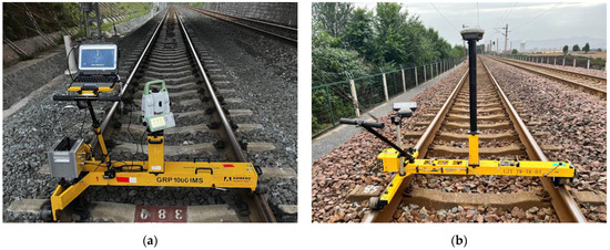
Figure 1. (a) INS trolley with TS configuration; (b) INS trolley with GNSS configuration.

Precise tamping with a heavy-duty machine is to guide heavy-duty track maintenance machinery to carry out digitally controlled tamping operations on ballasted tracks by using the measurement results. The tamping machine conducts track lifting, leveling, and alignment lining so as to improve the compactness of the track bed [8,9,10], and make the track geometry parameters meet the requirements of track design standards or maintenance codes [11], such as longitudinal level, cross level, and alignment of the track. At present, the main models of tamping machines used in China are the DCL-32 and DWL-48, which have some differences in the operating system, operation accuracy, and heavy-duty tamping machine parameter settings. DCL-32 [12] is a double-sleeper continuous tamping machine, which needs to be equipped with a dynamic track stabilizer, as is shown in Figure 2a. DWL-48 is a three-sleeper continuous tamping machine that integrates tamping and stabilization [13] and features high efficiency, high precision, and low energy consumption [14], as is shown in Figure 2b. DCL-32 and DWL-48 are produced using two tamping models produced by Plasser & Theurer as prototypes, which respectively include the 09-32 and 09-3X. Both the DCL-32 and DWL-48 models adopt Automatischer Leit Computer (ALC) control system and can achieve precise tamping. The stabilizing operation is used to simulate the stress state of the track under the action of the train, so as to achieve the purpose of re-compacting the ballast and avoiding uneven settlement of the track [15]. On-site maintenance personnel arrange the tamping machines and dynamic stabilizers appropriately to form different tamping modes for track maintenance operations.

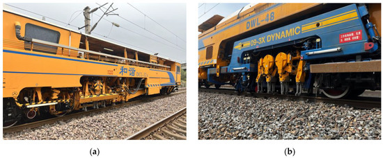
Figure 2. The main models of tamping machines: (a) DCL-32; (b) DWL-48.

The operation effect of different PMPT modes is affected by multiple factors. The degree of track geometry improvement depends on the track state before maintenance [16,17]. Different tamping operation modes have different effects on track geometry and track bed mechanical properties. Stabilizing operation will improve the track stability and extend the track quality warranty period [15]. Qu J. summed up the main factors affecting the tamping effect, which include the initial state of the tamping track, the measurement method, the tamping mode, the stabilizing operation, the models of the tamping machine, and the amount of lifting [1]. The condition of the track before the tamping operation affects the outcome of the tamping operation [18,19]. At present, there is no quantitative analysis method to determine the weight of the factors affecting the effect on the PMPT. The influence of different factors can only be qualitatively evaluated through field operation experience. We must use an optimal calculation method to quantify the influence weights of different factors and diagnosis the main factors affecting the effect on the PMPT. Scientifically guiding on-site construction operations and effectively improving the quality of operations are the pressing issues to be solved in the PMPT of ballast railways in China.

With the popularization and application of track inspection vehicles in China, a large amount of multi-source track inspection data has been accumulated, providing an important basis for track status evaluation. Neural networks can handle and analyze a huge amount of data, and even extract more data information from nonlinear data [20]. Machine learning technology has been widely applied in different fields, such as track status assessment [21], track geometry quality prediction [22,23], and railway fault diagnosis. In this study, the BPNN is selected because it is able to easily explore the importance of input features on output parameter. Therefore, having collected and sorted out the national-wide ballasted track PMPT maintenance statistics, the track inspection vehicle provides mega track geometry inspection data for the operation section. Based on the mega multi-source heterogeneous data and track geometry detection data, the BPNN is used to establish the main factor model that affects the PMPT operation effect. The influence weight of different factors on the PMPT effect is quantized for the first time, which is used to scientifically guide the control of key factors in the field operations. Some practical suggestions for the on-site application and operation mode optimization of the PMPT of the normal speed railway tracks are proposed, which provide a basis for reducing costs and increasing efficiency for heavy-duty track maintenance machinery operations, which has important practical significance and great economic benefits.

2. Related Work

2.1. The PMPT Operation Mode Database

From 2021 to 2022, a survey was carried out on the PMPT operation of national normal speed railway lines, and a database of the PMPT operation mode was established, which contains many actual on-site operations and track geometry inspection data, totaling about 27,000 km. The text data of the PMPT operation mode database includes the measurement method used before tamping, the model of the tamping machine, the tamping mode, the operation frequency of the stabilizer, etc. The conditional data includes whether it is with stabilizing operation, etc., and the digital data includes track geometry inspection data before and after tamping operation, improvement rate (IR), etc., among which various types of data contain data of different levels. The measurement methods mainly include INS trolley, INS trolley and CPⅢ, and INS trolley and GNSS. The tamping modes mainly include single tamping, single tamping and stabilizing, single pass double tamping and stabilizing, and single tamping and single tamping and stabilizing. The tamping machine models mainly include the DCL-32 and DWL-48. The operation frequency of the stabilizer mainly includes 0 Hz, 0–25 Hz and 25–40 Hz. On this basis, a scientific indicator system representing the main factors of PMPT operation effect was constructed.

2.2. Operation Effect Evaluation Index

The precise measuring and precise tamping operation are mainly used to improve the longitudinal level and the alignment irregularity of the track section by section so that the track profile of the line is constantly improved closer to the designed track profile. The study found that there was almost no change in track gauge before and after tamping operation, as is shown in Figure 3. In order to further improve the effectiveness of the operation effect evaluation index on the quality effect evaluation, the machine track quality index (MTQI) given in Equation (1) was used to the effect evaluation index. The cumulative distribution of the MTQI before and after tamping is shown as in Figure 4. It shows that there are obvious differences before and after the operation. The track geometry improvement before and after tamping is characterized by the track geometry improvement rate—which is expressed in Equation (2).

$$MTQI={\displaystyle \sum _{i=1}^6{\sigma }_i}$$

(1)

$$IR=\frac{MTQ{I}_{bf}-MTQ{I}_{af}}{MTQ{I}_{bf}}$$

(2)

where σ_i is the standard deviation of the 200 m inspection data of six track irregularities (i = 1, 2, …, 6), including the left and right longitudinal level, the left and right rail alignment lining, the cross level, and the twist; MTQI_bf is the MTQI before tamping, MTQI_af is the MTQI after tamping, and IR is the improvement rate of the MTQI.

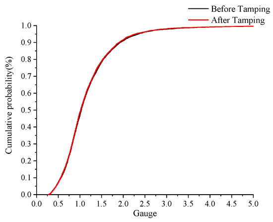
Figure 3. Cumulative distribution of track gauge before and after tamping.

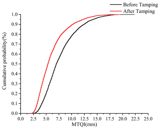
Figure 4. Cumulative distribution of MTQI before and after tamping.

2.3. Selection of Main Influencing Factors

Taking into consideration the actual operation and investigation on site, the main influencing factors that may exist in the whole process of PMPT operation were preliminarily determined. The quality of the track before tamping, MTQI_bf, the measurement method before tamping, the models of the tamping machine, the tamping mode, the frequency of stabilizing operation, and whether it had a stabilizer or not were input as the influencing factors. The input set X of the main factor model is defined as follows:

X = [X₁, X₂, X₃, X₄, X₅, X₆]

(3)

where X₁ is the measurement method before tamping. With the continuous progress of precise measurement technology, based on the different control network types, a variety of fast precise measurement methods were formed.

• X₂ is the tamping mode. There are four main tamping modes used in field operation, and different tamping modes have different quality effects after operation.
• X₃ is the model of the tamping machine. The main models of heavy-duty tamping machine used in China are the DWL-48 and DCL-32.
• X₄ is whether it has a stabilizer or not, which refers to whether there is stabilizing operation during the tamping operation.
• X₅ is the stabilizing operation frequency, which refers to the vibration frequency used in the stabilizing operation, which is mainly classified into 0 Hz (without stabilizing), 0~25 Hz, and 25~40 Hz. The compactness of the ballast bed after operation varies with different stabilizing operation frequencies [12].
• X₆ is track quality before tamping, MTQI_bf.

3. Model Building

The BPNN [24] is a multi-layer feedforward network trained based on the error back propagation algorithm. It uses the steepest descent method to continuously adjust the weights and thresholds of the network through back propagation to minimize the sum of squared errors of the network. The neural network structure diagram is shown in Figure 5.

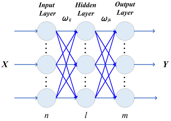
Figure 5. BPNN structure.

3.1. BPNN Training Model

Based on the data of different PMPT operation modes, a BPNN model was constructed by Matlab. By taking different influencing factors as inputs, the weights between each layer were calculated, and the weights of the influencing factors were obtained by statistics.

The main factor analysis model of the PMPT was characterized by the selection index system based on the influence of the PMPT effect. A huge amount of multi-source heterogeneous data was used as the input for the multi-layer feedforward neural network model. Through the transmission of signals between layers, the weighted connection of each neuron between the influencing factors of the input layer, the evaluation indicators of the hidden layer and the output layer were realized. The network weights and thresholds were adjusted based on the error of the predicted inspection data, and the cycle was repeated until a result meeting the error requirements was obtained. The network structure of the main factor analysis method that affected the PMPT operation effect is shown in Figure 6.

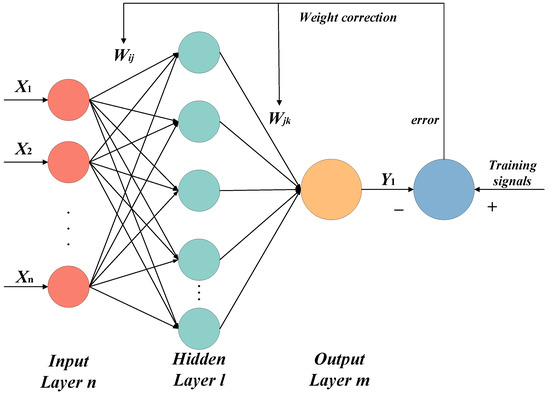
Figure 6. Neural network structure diagram by the main factor analysis method.

3.1.1. Statistical Index

MSE is the mean square error, as is shown in Equation (4). It calculates the expectation of the square of the difference between the true value y_i and the estimated value $\widehat{y}$_i. The smaller the MSE is, the better the model is. R is the correlation coefficient between the expected output and the actual output, as is shown in Equation (5). The closer the fitting slope of the expected output and the actual output is to 1, the better. k is the expected output and actual output fit slope, as is shown in Equation (6).

$$\mathrm{MSE}=\frac{1}{m}{\displaystyle \sum _{i=1}^m{(y_i-{\widehat{y}}_i)}^2}$$

(4)

$$R=\frac{{\displaystyle \sum _{i=1}^n\left(y_i-\overline{y}\right)\left({\widehat{y}}_i-\overline{\widehat{y}}\right)}}{\sqrt{{\displaystyle \sum _{i=1}^n{\left(y_i-\overline{y}\right)}^2}}\sqrt{{\displaystyle \sum _{i=1}^n{\left({\widehat{y}}_i-\overline{\widehat{y}}\right)}^2}}}$$

(5)

$$k=\frac{{\displaystyle \sum _{i=1}^n{y}_i{\widehat{y}}_i-n\overline{y}\overline{\widehat{y}}}}{{\displaystyle \sum _{i=1}^n{y}_i{}^2-n{\overline{y}}^2}}$$

(6)

3.1.2. Selecting Model Parameters

In the original data, the initial quality of the track (MTQI_bf), the measurement method before tamping, the model of the tamping machine, the tamping mode, whether it had a stabilizer, and the frequency of stabilizing operation were processed as the input layer. The number of nodes in the input layer of the network was six (n = 6). The track quality after tamping (MTQI_af) or the IR was used as the output layer. The number of nodes in the output layer of the network was one (m = 1).

A network, with bias and at least one sigmoid hidden layer plus a linear output layer, is capable of approximating any rational function. Increasing the number of layers can further reduce the error and improve the accuracy; however, it also complicates the network. The parameter configuration of the neural network requires multiple attempts to adjust different parameters to determine the activation function of the hidden layer and the number of neurons in the hidden layer. By evaluating the network indicators with the correlation coefficient R, the fitting slope k and the value of MSE, a relatively good combination method can meet the principal factor analysis of the PMPT model was selected. The relatively optimal combination is shown as in Table 1 and Table 2.

Table 1. Both input and output normalized fitting results.

Output Layer	Hidden Layer	The Number of Neurons in Hidden Layer	R	k	MSE
purelin	sigmoid	10	0.80841	0.655	1.38917
		20	0.81167	0.665	1.36820
		30	0.81265	0.667	1.36610
		50	0.81387	0.669	1.35414
	poslin	10	0.79767	0.636	1.45859
		20	0.80408	0.646	1.41714
		30	0.80706	0.649	1.40782
		50	0.81117	0.662	1.37169
	purelin	10	0.74900	0.561	1.76048
		20	0.74897	0.555	1.76073
		30	0.74902	0.557	1.76050
		50	0.74906	0.560	1.75990
	tansig	10	0.80639	0.652	1.40226
		20	0.81199	0.665	1.36627
		30	0.81201	0.665	1.36635
		50	0.81211	0.666	1.36640

Table 2. Input normalized, output unnormalized fitting result.

Output Layer	Hidden Layer	The Number of Neurons in Hidden Layer	R	k	MSE
purelin	sigmoid	10	0.81044	0.659	1.37633
		20	0.81307	0.667	1.35926
		30	0.81328	0.667	1.35872
		50	0.81342	0.670	1.35720
	poslin	10	0.79514	0.635	1.47453
		20	0.80393	0.647	1.41840
		30	0.80452	0.650	1.40821
		50	0.80960	0.654	1.38164
	purelin	10	0.74893	0.561	1.76071
		20	0.74890	0.563	1.76096
		30	0.74893	0.561	1.76080
		50	0.74895	0.562	1.76067
	tansig	10	0.80783	0.657	1.39301
		20	0.81267	0.662	1.36202
		30	0.81398	0.665	1.35420
		50	0.81427	0.665	1.35219

Table 1 and Table 2 show that, when the training results of the neural network are relatively good, the parameters of the neural network are set as follows (as is shown in Figure 7):

a.

The number of neurons in the hidden layer: l = 30. Selecting 30 hidden layers not only makes the results more accurate, but also has high computational efficiency.

b.

Input normalized; output not normalized;

c.

Hidden layer activation function: tansig;

d.

Output layer activation function: purelin;

e.

The learning rate of the BPNN is set to 0.01;

f.

The epoch of the BPNN is set to 100.

Figure 7. Neural network training structure.

3.1.3. Model Training Step

The training steps of the model are as follows:

Step 1: Calculate the output value H of the hidden layer according to the influencing factors of the input layer X, calculate the connection weight ω_ij between the input layer and the hidden layer, and calculate the threshold α of the hidden layer.

$$H_j=f\left({\displaystyle \sum _{i=1}^n{\omega }_{ij}{x}_i-{\alpha }_j}\right)\begin{array}{cc}& j=1,2,\cdots ,l\end{array}$$

(7)

where l is the number of hidden layers at 30; and f is the activation function tansig of the hidden layer.

Step 2: According to the output value H of the hidden layer, the connection weight ω_jk and threshold b between the hidden layer and the output layer, calculate the O of the BPNN to predict the output of the MTQI_af or IR.

$$O_k={\displaystyle \sum _{j=1}^l{H}_j{\omega }_{jk}}-b_k\begin{array}{cc}& k=1,2,\cdots ,m\end{array}$$

(8)

Step 3: Calculate the network prediction error e according to the network prediction output O and the expected output value Y.

$$e_k=o_k-y_k\begin{array}{cc}& k=1,2,\cdots ,m\end{array}$$

(9)

Step 4: According to the network prediction error e, update the weights ω_ij and ω_jk between the layers of the network, as well as the new network node thresholds α and b.

$${\omega }_{ij}={\omega }_{ij}+\eta H_j\left(1-H_j\right)x\left(i\right){\displaystyle \sum _{k=1}^m{\omega }_{jk}{e}_k}\begin{array}{cc}& i=1,2,\cdots ,n;j=1,2,\cdots ,\end{array}l$$

(10)

$${\omega }_{jk}={\omega }_{jk}+\eta H_j{e}_k\begin{array}{cc}& j=1,2,\cdots ,l;k=1,2,\cdots ,\end{array}m$$

(11)

Step 5: Determine whether the iteration of the model algorithm has reached its end; if not, go back to Step 1.

3.2. Abnormal Data Cleaning

Due to the random error in the data set, in order to further improve the fitting effect of the model, on the basis of the established BPNN prognosis model, it was necessary to clean the data of the PMPT modes. We calculated the standard deviation of the actual error value of the predicted output value (estimated by the 1/2 power of the sample variance), removed the samples exceeding 3σ, and retrained until the data MSE stabilized.

$$\left|e_i-\mu \right|>3\sigma$$

(12)

where μ is the mean error; and σ is the error standard deviation.

We iteratively cleaned n times until the number of cleanings had little effect on the R, MSE, and the amount of data that was cleaned.

3.3. Calculation Method of Influence Factor Weight

The weight associated with each feature conveys the importance of the feature in predicting the output value, so the weight is used to represent the influence of each factor on the quality of the track work after tamping.

Note that the weight w of the hidden layer is iiw in Equation (13), and the weight of the output layer is llw in Equation (13). The input data matrix is n × m dimensional: m is the amount of data. There are 30 hidden layer neurons, so the hidden layer weight iiw is a n × 30 dimensional matrix, and the output layer weight llw is a 30 × 1 dimensional matrix. Use the product of iiw and llw (n × 1 dimensional matrix) as the weight for the n factors in the corresponding input. The weight formula of influencing factors is shown in Equation (14).

$$\{\begin{array}{c}iiw=net.IW\left\{1,1\right\}\\ llw=net.LW,\left\{2,1\right\}\end{array}$$

(13)

$$W_1=iiw\times llw$$

(14)

Due to the defects of the standard BP algorithm, it is easy to form a local minimum that does not obtain a global optimal solution. Therefore, the neural network model with the same structure was repeatedly trained 10,000 times on the cleaned training data, and the network weight in Equation (14) or its related form each time, as well as the ranking value of each factor weight each time, which was recorded for subsequent statistical processing.

4. Case Analysis

Taking the PMPT data of the national conventional speed lines as an example, the overall process of using the BPNN to study the effect of different influencing factors on the effect of the heavy-duty tamping machine is mainly classified into the following steps, as shown in Figure 8:

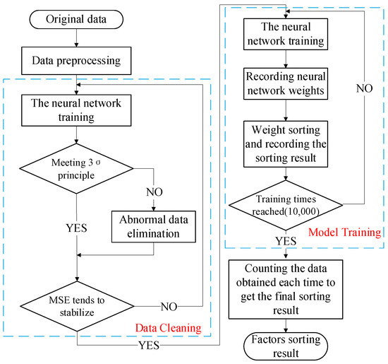
Figure 8. Overall flowchart.

4.1. Original Data Source

Local railway administrations in our country provide the operation information of the ballasted track PMPT maintenance section on the conventional speed railway every month, including the line, line type, operation start and end mileage, tamping date, measurement method, tamping mode, tamping machine model, stabilizer vibration frequency etc. Track inspection vehicles or comprehensive inspection trains are used to inspect the track geometry of the operating railway in China. Different speed grade lines have different inspection frequencies. The more important the line grade is, the higher the inspection frequency is. It is mainly divided into once a month, once every 20 days, or twice a month. Therefore, the track geometry inspection data of national railway lines were possessed. According to the maintenance information, the latest inspection data before and after tamping operation are matched from the inspection database as the MTQI_bf and MTQI_af, respectively. Part of the original data is shown in Table 3.

Table 3. Part of original data.

Measurement Method	Tamping Machine Model	Tamping Mode	Stabilized Track	Stabilizer Vibration Frequency	MTQIbf/mm	MTQIaf/mm	IR (%)
INS Trolley	DCL-32	single tamping and single tamping and stabilizing	Yes	0~25 Hz	4.9	4.7	4.1
INS Trolley	DWL-48	single pass double tamping and stabilizing	Yes	25~40 Hz	8.6	7.1	17.4
INS Trolley and GNSS	DCL-32	single tamping	No	0 Hz	3.5	2.5	28.6
INS Trolley and GNSS	DWL-48	single tamping and stabilizing	Yes	25~40 Hz	3.4	2.5	26.5
INS Trolley and CPⅢ	DCL-32	single pass double tamping and stabilizing	Yes	0~25 Hz	5.9	4.4	25.4
INS Trolley and CPⅢ	DWL-48	single tamping	No	0 Hz	6.3	5.3	15.9

4.2. Data Preprocessing

In the data preprocessing stage, each factor level number and combined data screening are performed on the original data (Table 3). The specific process is as follows:

Using the neural network for regression analysis, it identifies the variables with significant influence from multiple variables that affect a variable and uses the obtained relational expression to estimate or predict another specific variable based on the value of one variable or multiple variables. The influence of each factor on the quality of the track after tamping is studied, so the numbering method is used to number each factor and each level, and each factor is used as the input, as is shown in Table 4. The data form of MTQI or IR after tamping is the target value.

Table 4. Input factor corresponding coding example.

Code	1	2	3	4
Tamping mode	single tamping	single tamping + stabilizing	single pass double tamping and stabilizing	single tamping and single tamping and stabilizing
Measurement method	INS Trolley	INS Trolley and GNSS	INS Trolley and CPⅢ	-
Stabilizer vibration frequency	0 Hz	25~40 Hz	0~25 Hz	-
Tamping machine model	DCL-32	DWL-48	-	-
Stabilized track	No	Yes	-	-

4.3. Data Cleaning

Figure 9 shows the R, MSE, and the data that was cleaned away with the change in the number of cleanings. The total amount of known data was 30,022. A total of about 1800 pieces of data were cleaned. As the number of cleaning times increased, the correlation coefficient became bigger, and the MSE gradually became smaller and stable. The number of cleaning times was set 100. If the cleaning effect was not ideal, and, moreover, Figure 8 shows that increasing the cleaning number did not improve the cleaning effect, then the range of effective data could be accurately determined by reducing 3σ in Equation (12).

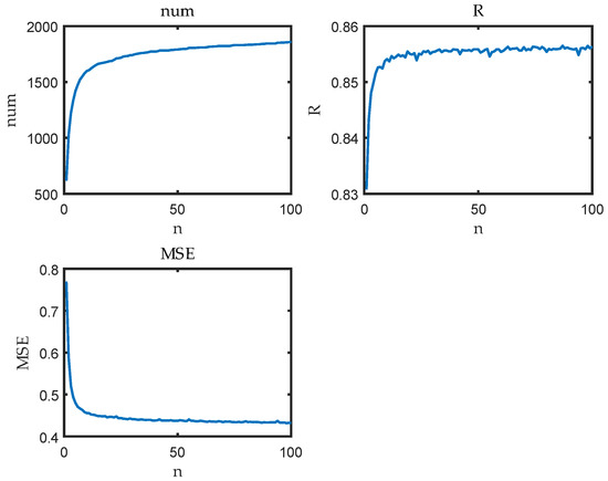
Figure 9. Data changes with the number of cleaning.

4.4. Neural Network Training

4.4.1. Splitting the Dataset

We split the dataset into a training set, validation set, and test set. Among them, the training set was used to train the neural network model; the validation set came from the subdivision of the training set, which was used for model selection and parameter adjustment; the test set was used to test the identification ability of the learner for new samples, and the test error was used as the generalization error. The approximate value of the data set was divided into 70% for the training set, 15% for the validation set, and 15% for the test set.

4.4.2. Model Training

The maximum number of iterations allowed in the model epoch was set to 100. The system stops when it reaches the training goal or reaches the maximum number of iterations. Figure 10 respectively shows the performance of the MSE metrics for the BP training, validation, and testing processes in each generation. The figure shows that the MSE decreased with the increase in the number of iteration rounds. The best verification performance was 0.44533 in the 7th round, and it tended to be stable. The training ended after 13 rounds.

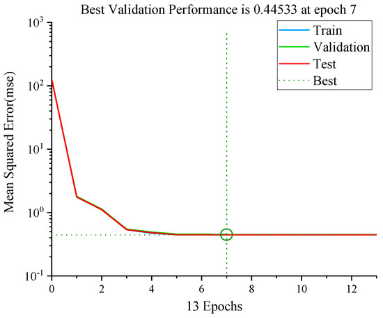
Figure 10. Performance of MSE indicators in each generation.

4.4.3. Evaluation Index

In this paper, the coefficient of determination R (Equation (5)) was adopted to evaluate the effectiveness of the model. The coefficient of determination R was close to 1, indicating that the trained network model was trained well. Meanwhile, the median absolute deviation (MAD) and mean absolute percentage error (MAPE) evaluation indicators were used to aid the evaluation of the prognosis effectiveness of the target value. The foregoing define the deviation between the predictive value and true value, thus reflecting the prognosis capacity. The lower the error value, the better the prognosis effect and the higher the accuracy of the target data. The calculation formula is:

$$\{\begin{array}{c}MAD=median\left(\left|{\upsilon }_i-{\upsilon }_m\right|\right)\\ MAPE=\frac{100\%}{n}{\displaystyle \sum _{i=1}^n\left|\frac{{\widehat{y}}_i-y_i}{y_i}\right|}\end{array}$$

(15)

where υ_i is the i th value of $\widehat{y}-y$, υ_m is the median value of υ, and n is the amount of data.

Figure 11 is the result of fitting the target value of each dataset with the estimated value of the neural network. After experimentation, the data results after cleaning were trained based on the above structural neural network model. The correlation coefficient R could reach about 0.85 when the target value was the MTQI_af. When the target value was the IR, R was only about 0.5. It shows that the neural network can fit MTQI_af well, but the processing effect of IR is not satisfactory. Therefore, the MTQI_af was selected as the only output of the neural network model. After 10,000 trainings, the mean of the MSE was 0.432, as is shown in Figure 12; the mean of the MAD was 0.64, as is shown in Figure 13; and the mean of the MAPE was 13.2%, as is shown in Figure 14. It can be seen that the deviation was small and the prediction effect was good. They met our precision needs for this study.

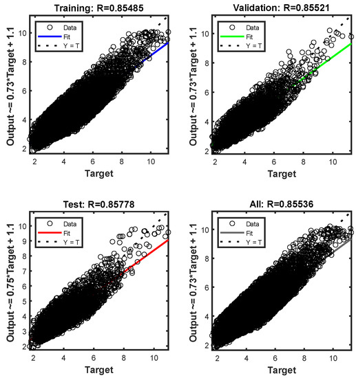
Figure 11. The fitting effect of the model training on the target value MTQI_af.

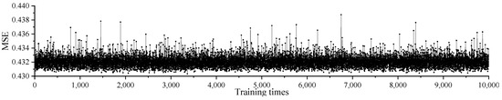
Figure 12. The MSE of MTQI_af.

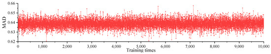
Figure 13. The MAD of MTQI_af.

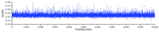
Figure 14. The MAPE of MTQI_af.

4.5. Result

Statistical methods for the research results were affected by various factors and include the follow steps:

Sort the weights of each factor obtained by each training model, record the sorting value of each training 10,000 times, find the mean of the sorting value of each factor, and finally sort the obtained sorting mean to get the final sorting result of each factor.

As is shown in Figure 15, the horizontal axis represents the ranking of weights (from small to big), and the vertical axis represents the probability of the corresponding weights of each influencing factor during 10,000 times of training. For example, the MTQI_bf was 0.0341 at weight 1 and 0.3847 at weight 6. The weighted average value of the weighted sorting value (Equation (16)) was taken as the weight of each influencing factor, which was sorted from the biggest to the smallest, as is shown in Table 5. The statistical results show that the order of factors influencing the effect of tamping was the MTQI_bf, stabilized track or not, tamping mode, stabilizer vibration frequency, measurement method, and tamping machine model.

$$AS={\displaystyle \sum _{i=1}^6{\omega }_i}{S}_i$$

(16)

where AS is the average sort of influencing factors, ω_i is the statistical probability, and S_i is the weight sorting (S_i = 1, 2, …, 6).

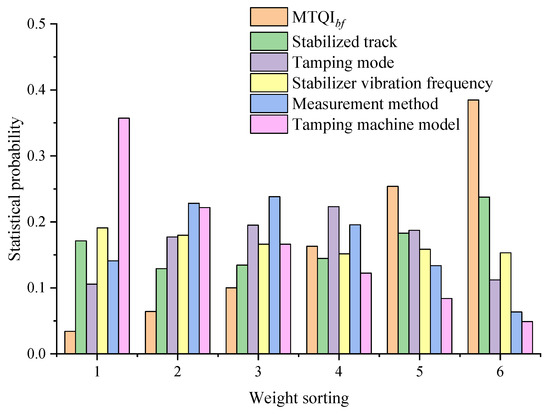
Figure 15. Distribution of weight ranking of each influencing factor.

Table 5. Influencing factor weighted statistics results.

	Factors	MTQIbf	Stabilized Track	Tamping Mode	Stabilizer Vibration Frequency	Measurement Method	Tamping Machine Model
Weight Sorting
1		0.0341	0.1713	0.1055	0.1909	0.1410	0.3572
2		0.0641	0.1291	0.1772	0.1798	0.2282	0.2216
3		0.1001	0.1345	0.1950	0.1661	0.2382	0.1661
4		0.1631	0.1446	0.2230	0.1515	0.1955	0.1223
5		0.2539	0.1829	0.1872	0.1585	0.1336	0.0839
6		0.3847	0.2376	0.1121	0.1532	0.0635	0.0489
Average sort		4.6927	3.7515	3.5455	3.3665	3.1430	2.5008
Order		1	2	3	4	5	6

5. Discussions

In this paper, the method of deep learning was used to study the main factors on the effect of the PMPT. Through the testing and training model, the BPNN could better fit the influence of various factors on the MTQI_af and obtain the weight of factors. The determination of factors is intended to solve the actual problems of field operation, so it is necessary to reconcile the field operation experience.

When the track quality before tamping is poor, tamping operation can significantly improve the track quality, but when the track quality before tamping is good, tamping operation has little effect on improving the track quality. Therefore, the initial quality of the line has an obvious impact on the tamping effect. The stabilizing operation can rearrange and compact the ballast particles under the sleeper, improve the stability, and restore the bearing capacity of the ballast bed. The different times of inserting picks in the tamping mode affect the ballast arrangement, the compactness of the ballast bed, and the track geometry. In addition, the accuracy of measurement equipment, the operating parameters of the heavy-duty machine, and the tamping machine model also affect the tamping effect. The result obtained by the model accords with the actual situation of the field.

The main factors affecting the effect of the PMPT were clarified, which can scientifically guide the field personnel to strictly control the key links of PMPT. It provides references for the selection of tamping mode, tamping machine model, measurement method, and other operation mode, as well as puts forward some practical suggestions for promoting the application of the PMPT of railway conventional speed lines. It has important practical significance and huge economic benefits to provide a basis for cost reduction and the efficient increase of heavy-duty track maintenance machinery operation.

6. Conclusions

In this paper, through the collection and processing of field data in recent two years, the database of the PMPT operation mode was structured and constructed. The selection index system of the influence of on-site PMPT effects based on big data was established. Based on many multi-source heterogeneous data and track geometry detection data, BPNN technology was used for the first time to select the number of output layers, hidden layer activation functions, and hidden layer neurons that met the characteristics of the data, and it established the main factor model that affected the PMPT operation effect. The accuracy of the neural network model was improved through abnormal data cleaning. The quantitative order of factors influencing the effect of the PMPT were the MTQI_bf, stabilized track or not, tamping mode, stabilizer vibration frequency, measurement method, and tamping machine model.

References

- Qu, J. Research on Prediction Method of Warranty Period of Track Quality Based on Tamping Modes Using Large Tamping Machine. J. China Railw. Soc. 2019, 41, 117–122. [Google Scholar] [CrossRef]
- Khouy, I.A.; Larsson-Kråik, P.-O.; Nissen, A.; Juntti, U.; Schunnesson, H. Optimisation of track geometry inspection interval. Proc. IMechE Part F 2014, 228, 546–556. [Google Scholar] [CrossRef]
- Martey, E.; Attoh-Okine, N. Modeling tamping recovery of track geometry using the copula-based approach. Proc. IMechE Part F 2018, 232, 2079–2096. [Google Scholar] [CrossRef]
- Chen, Q.; Niu, X.; Zuo, L.; Zhang, T.; Xiao, F.; Liu, Y.; Liu, J. A Railway Track Geometry Measuring Trolley System Based on Aided INS. Sensors 2018, 18, 538. [Google Scholar] [CrossRef] [PubMed]
- Sánchez, A.; Bravo, J.L.; González, A. Estimating the Accuracy of Track-Surveying Trolley Measurements for Railway Maintenance Planning. J. Surv. Eng. 2017, 143, 05016008. [Google Scholar] [CrossRef]
- Luo, Y.; Liu, C.; Yang, X.; He, Y.; Song, T. A New Method for Establishment of Plane Network of Ordinary Conventional-speed Railway Track Control Network and its Accuracy Discussion. J. Railw. Sci. Eng. 2014, 11, 55–59. [Google Scholar] [CrossRef]
- Chen, Q.; Niu, X.; Zhang, Q.; Cheng, Y. Railway Track Irregularity Measuring by GNSS/INS Integration. Navigation 2015, 62, 83–93. [Google Scholar] [CrossRef]
- Nielsen, J.C.; Berggren, E.G.; Hammar, A.; Jansson, F.; Bolmsvik, R. Degradation of railway track geometry–Correlation between track stiffness gradient and differential settlement. Proc. IMechE Part F 2020, 234, 108–119. [Google Scholar] [CrossRef]
- Zhang, M.N.; Wu, Y.B.; Ma, X.C.; Wang, P. Influence of Large Track Maintenance Machine on Sleeper Supporting Stiffness. Adv. Mat. Res. 2014, 919–921, 1115–1119. [Google Scholar] [CrossRef]
- Zhou, T.Y.; Hu, B.; Yan, B.; Peng, Y.X. Study on Motion Parameters of Tamping Operation. Adv. Mat. Res. 2013, 694–697, 154–157. [Google Scholar] [CrossRef]
- Rhayma, N.; Bressolette, P.; Breul, P.; Fogli, M.; Saussine, G. Reliability analysis of maintenance operations for railway tracks. Reliab. Eng. Syst. Saf. 2013, 114, 12–25. [Google Scholar] [CrossRef]
- Wang, X.J.; Geng, X.L. Study on the Effects of Tamping Frequency to the Compaction Degree of Trackbeds. Appl. Mech. Mater. 2012, 178–181, 1387–1391. [Google Scholar] [CrossRef]
- Zhou, T.Y.; Hu, B.; Wang, X.J.; Yan, B. Discrete Element Method Analysis of Mechanical Properties of Railway Ballast during Tamping Process under Different Amplitude. Appl. Mech. Mater. 2012, 233, 224–227. [Google Scholar] [CrossRef]
- Guo, Y.; Markine, V.; Jing, G. Review of ballast track tamping: Mechanism, challenges and solutions. Constr. Build. Mater. 2021, 300, 123940. [Google Scholar] [CrossRef]
- Jadidirendi, K.; Zakeri, J.A.; Teng, H. Field Investigation for Identifying the Effects of Dynamic Track Stabilizing Operation on Track Geometrical Indices. In Proceedings of the 2015 Joint Rail Conference, San Jose, CA, USA, 23–26 March 2015. [Google Scholar] [CrossRef]
- Selig, E.; Waters, J. Track Geotechnology and Substructure Management; Thomas Telford: London, UK, 1994; Available online: https://www.icevirtuallibrary.com/doi/book/10.1680/tgasm.20139 (accessed on 20 October 2022).
- Esveld, C. Modern Railway Track; MRT-Productions Zaltbommel: Zaltbommel, The Netherlands, 2001. [Google Scholar]
- Offenbacher, S.; Koczwara, C.; Landgraf, M.; Marschnig, S. A Methodology Linking Tamping Processes and Railway Track Behaviour. Appl. Sci. 2023, 13, 2137. [Google Scholar] [CrossRef]
- Neuhold, J. Tamping within Sustainable Track Asset Management; Verlag der Technischen Universität Graz: Graz, Austria, 2020. [Google Scholar]
- Khajehei, H.; Ahmadi, A.; Soleimanmeigouni, I.; Haddadzade, M.; Nissen, A.; Jebelli, M. Prediction of track geometry degradation using artificial neural network: A case study. Int. J. Rail. Trans. 2022, 10, 24–43. [Google Scholar] [CrossRef]
- Sadeghi, J.; Askarinejad, H. Application of neural networks in evaluation of railway track quality condition. J. Mech. Sci. Technol. 2012, 26, 113–122. [Google Scholar] [CrossRef]
- Sresakoolchai, J.; Kaewunruen, S. Track Geometry Prediction Using Three-Dimensional Recurrent Neural Network-Based Models Cross-Functionally Co-Simulated with BIM. Sensors 2023, 23, 391. [Google Scholar] [CrossRef] [PubMed]
- Shafahi, Y.; Masoudi, P.; Hakhamaneshi, R. Track Degradation Prediction Models, Using Markov Chain, Artificial Neural and Neuro-Fuzzy Network. In Proceedings of the 8th World Congress on Railway Research, Seoul, Republic of Korea, 18–22 May 2008; pp. 1–9. Available online: https://www.researchgate.net/publication/268011897 (accessed on 12 March 2023).
- LeCun, Y.; Bengio, Y.; Hinton, G. Deep learning. Nature 2015, 521, 436–444. Available online: https://www.nature.com/articles/nature14539 (accessed on 20 October 2022). [CrossRef] [PubMed]
Disclaimer/Publisher’s Note: The statements, opinions and data contained in all publications are solely those of the individual author(s) and contributor(s) and not of MDPI and/or the editor(s). MDPI and/or the editor(s) disclaim responsibility for any injury to people or property resulting from any ideas, methods, instructions or products referred to in the content. |
© 2023 by the authors. Licensee MDPI, Basel, Switzerland. This article is an open access article distributed under the terms and conditions of the Creative Commons Attribution (CC BY) license (https://creativecommons.org/licenses/by/4.0/).