Study on Beat Vibration of a High Temperature Superconducting EDS Maglev Vehicle at Low Speed

Abstract

Vertical displacement acceleration and the pitch angle record produce the phenomenon of beat vibration when testing a 200 m electro-dynamic suspension (EDS) magnetic levitation (maglev) test vehicle with high-temperature superconducting (HTS) at the CRRC Changchun Railway Vehicles Co., Ltd., where the vehicle is clamped and in planar motion. First, to examine this phenomenon, this paper establishes dynamic equations of the vehicle with three degrees of freedom (DOF), and the levitation force on each superconducting magnet (SCM) is calculated by dynamic circuit theory. Second, the theory vertical equilibrium point is obtained from the average of the levitation force for a different velocity and the magneto-motive force (MMF) of the SCM. Third, this paper decouples SCM levitation forces from each other using MATLAB/SIMULINK, and a multi-body dynamic model with six DOF is developed in SIMPACK. All vertical displacements and acceleration responses, as well as the pitch angle and acceleration response from the simulation, appear to show the phenomenon of beat vibration since there are two closing natural frequencies of approximately 2 Hz and 2.4 Hz. Finally, based on the traversing method considering the influence of the velocity, initial vertical displacement, and the MMF of the SCM, the multi-body dynamic model is frequently utilized to study the response of the mean and amplitude of vertical displacement and that of the pitch angle. The results show that increasing the MMF or velocity could decrease the vertical displacement and pitch angle; the mean vertical displacement is a little larger than the theory equilibrium point; and the amplitude of vertical displacement is small when the initial vertical displacement is near the theory equilibrium point. Both the numerical and experimental results verify the validity of the dynamic circuit model and mechanical model in this paper.

1. Introduction

A maglev (magnetic levitation) train can travel along tracks without mechanical contact with the ground; it has the advantages of high speed, low noise, low carbon emissions, and a high degree of safety to meet the requirements of future transportation systems [1,2,3,4,5,6,7,8,9,10,11,12,13,14,15,16,17,18,19]. Various maglev systems, including electro-magnetic suspension (EMS), electro-dynamic suspension (EDS), and high-temperature superconducting (HTS) pinning maglev, have been developed and tested in Germany, Japan, South Korea, and China for more than 50 years [1,2,3,4,5,6]. The EDS system was introduced by J. R. Powel and G.T. Dan [7], where null-flux figure-eight-shaped coils were built on both sides of the guideway for levitation and guidance. EDS trains have large suspension air-gaps of above 10 cm compared with EMS trains; they also have a better running safety when climbing, going downhill, or under subgrade deformation [8,9,10]. The low-temperature superconducting magnet–null-flux coil EDS system was first developed in Japan in the 1980s [8,9]. Thanks to the efforts of Japanese scientists, the JR maglev was found to be able to travel at a high speed of approximately $603\hspace{0.33em}\mathrm{kmph}$ in 2015. A large amount of research has been carried out to study the dynamic performance of the JR maglev system [8,9,10,11,12,13,14,15,16]. Shunsuke Ohashi [9] studied the mechanical model of the EDS system based on the dynamic circuit theory. Since the damping is too small, efforts were also carried out to improve the damping effect [10,11]. Because a guideway will always be used, experts should also consider the dynamic interaction between a vehicle and guideway [12,13,14]. At the same time, experts should also study a vehicle’s dynamic performance under accident conditions, such as with a quenched SC coil [15,16], and conduct enough running tests [17] to guarantee the vehicle’s safety. Generally, the levitation force, guiding force, and drag force, which are generated between ground coils on the ground and the SCM on board, are dependent on the velocity and position of a vehicle [18,19] and other electric parameters.

When predicting a vehicle’s dynamic performance, there are two methods which are commonly used. The first method to determine the vertical performance is based on vibration theory with one degree of freedom (DOF) [9], where the magnetic force is calculated first. However, with this method, the pitch angle of a vehicle is ignored. To overcome this shortcoming, the second method [13] considers the full dynamic coupling of magnetic forces, the current, the magnetic field, the movement of a vehicle, and even flexible bodies. However, the calculation of these forces is quite time consuming.

Recently, the CRRC Changchun Railway Vehicles Co., Ltd. (Changchun, China) developed a new 200 m straight test line with a high-temperature superconducting EDS maglev vehicle, as shown in Figure 1, unlike the Japanese low-temperature superconducting EDS maglev vehicles. There are eight HTS fixed on both sides of the vehicle. To solve any practical problems in the whole system from low velocity to high velocity step by step, a test vehicle was designed to run at a low velocity of approximately 14 mps to ensure the vehicle’s safety. When all problems are solved at a low velocity, the test line can then be upgraded to run at a higher speed to uncover the new phenomenon of the system. It is particularly difficult to make the vehicle run at a rated velocity because the experimental test is limited by the traction system, current SCM, initial vertical displacement, and so on. The vehicle is clamped by four guiding wheels and is in a planar motion. When running at 13.7 m/s (mps), both the vertical displacement acceleration and pitch angle show the phenomenon of beat vibration, as shown in Figure 2. Currently, experimental records show this unexpected phenomenon of beat vibration, which has not yet been reported in other literature despite the low velocity value. In other words, only researching vertical displacement is incorrect. This phenomenon is caused by vehicle and complex magnetic forces together, so it may also appear in some other maglev vehicles, but it is a specific problem of this test vehicle that needs to be solved. It is useful and helpful to uncover this phenomenon for future research. Therefore, this paper provides a method to simulate this unexpected phenomenon. At the same time, we use numerical results and experimental phenomenon to verify the validity of the dynamic circuit model, the mechanical model, and the method to treat the magnetic force.

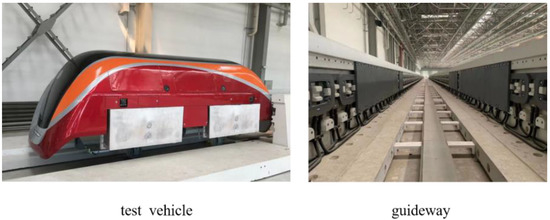
Figure 1. The 200 m straight EDS maglev test line with high-temperature superconducting (HTS) at the CRRC.

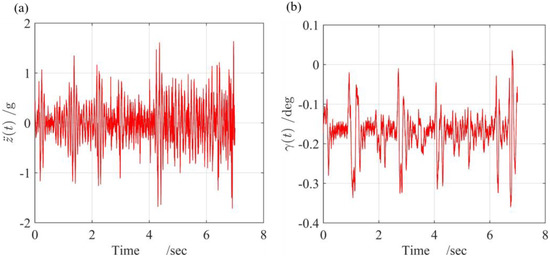
Figure 2. Experimental running results when $v=13.7\hspace{0.33em}\mathrm{mps}$: (a) vertical displacement acceleration $\ddot{z}(t)$; (b) pitch angle $\gamma (t)$.

To uncover the phenomenon of beat vibration, this paper set up governing equations of a vehicle with three DOF. First, the levitation forces were calculated by the dynamic circuit theory with the different velocity, vertical displacement, and magneto-motive force (MMF) of a superconducting magnet (SCM). The theory vertical equilibrium point was calculated as in Ref. [9]. A new multi-body dynamic model was developed in SIMPACK script, where the levitation force was exchanged in MATLAB/SIMULINK with the aid of the tool MATSIM. Finally, considering the influence of the velocity, initial vertical displacement, and the MMF of the SCM, based on the traversing method, the vertical displacement and pitch angle were examined. The main contributions of this paper are that the levitation forces on each SCM are decoupled from each other and the simulation results successfully uncover the phenomenon of beat vibration.

2. Governing Equations

2.1. Definition of Two Coordinate Systems

Two coordinate systems, the inertial reference $o-xyz$ and the body coordinate system $O-XYZ$ on the vehicle, are used to describe the motion of the vehicle, as shown in Figure 3. Generally, six variables describing the relative motion between the vehicle and the inertial reference are the longitudinal position $x(t)$, vertical position $z(t)$, lateral position $y(t)$, roll angle $\phi (t)$, yaw angle $\psi (t)$, and pitch angle $\gamma (t)$.

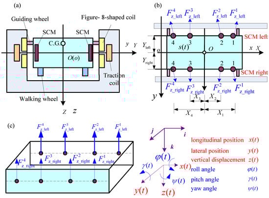
Figure 3. Sketch and force diagram of test line with SCM coils and ground coils at the CRRC: (a) cross section; (b) vertical view; (c) eight levitation forces.

With the inertial reference $o-xyz$, the origin is in the middle of the plane defined by the figure-eight-shaped coils; the $i$ direction of the longitudinal position $x$ is along the track; the $k$ direction of the vertical position $z$ is downward as the direction of gravity of the acceleration; and the $j$ direction of the lateral position $y$ is defined by $j=k\times i$. The ground figure-eight-shaped coils are equally spaced along both sides of the track with a pole pitch of $pitch=0.36\hspace{0.33em}\mathrm{m}$. The locations of the left figure-eight-shaped coils and the right figure-eight-shaped coils satisfy Equations (1) and (2):

$$y_{\mathrm{left}\_\mathrm{figure}\_8}=-y_0,\hspace{1em}{z}_{\mathrm{left}\_\mathrm{figure}\_8}=0\hspace{1em}\hspace{1em}(\mathrm{figure}-\mathrm{eight}-\mathrm{shaped} \mathrm{coils}\hspace{0.17em}\mathrm{on} \mathrm{left} \mathrm{side})$$

(1)

$$y_{\mathrm{right}\_\mathrm{figure}\_8}=y_0,\hspace{1em}{z}_{\mathrm{right}\_\mathrm{figure}\_8}=0\hspace{1em}\hspace{1em}(\mathrm{figure}-\mathrm{eight}-\mathrm{shaped} \mathrm{coils}\hspace{0.17em}\mathrm{on} \mathrm{right} \mathrm{side})$$

(2)

where $y_{\mathrm{left}\_\mathrm{figure}\_8}$ and $y_{\mathrm{right}\_\mathrm{figure}\_8}$ are the lateral positions of the left figure-eight-shaped coils and the right figure-eight-shaped coils, respectively; $z_{\mathrm{left}\_\mathrm{figure}\_8}$ and $z_{\mathrm{right}\_\mathrm{figure}\_8}$ are the vertical positions of the left and right figure-eight-shaped coils, respectively; and $y_0$ is the constant.

The body coordinate system $O-XYZ$ fixed on the vehicle is defined by the following method. First, each base vector of the body coordinate system is initially parallel with the corresponding base vector of the inertia reference. The origin of the body coordinate system is not at the center of gravity (C.G), but rather it is at the geometric center of the plane, defined by the center lines of the SCMs on both sides of the vehicle, as shown in Figure 3. The reason is that when plane $O-XY$ coincides with plane $o-sy$, there is no magnetic force when the vehicle is moving forward.

2.2. Dynamic Equations of the Vehicle

The HTS test vehicle is clamped by four guiding wheels in contact with the sidewall and it is within the planar motion. The vehicle has three independent DOFs: $x(t)$, $z(t)$ and $\gamma (t)$. The inertial parameters of the vehicle on the C.G are shown in Table 1. The vehicle is symmetric on planes $O-XZ$ and $O-YZ$, and the location of the C.G is $[0,0,Z_{\mathrm{C}.\mathrm{G}.}]$, where $Z_{\mathrm{C}.\mathrm{G}.}=-0.118\hspace{0.33em}\mathrm{m}$. The location of the C.G in the inertial reference can be described by Equations (3)–(5):

$$s_{\mathrm{C}.\mathrm{G}.}(t)=s(t)+Z_{\mathrm{C}.\mathrm{G}.}\sin \gamma (t)$$

(3)

$$y_{\mathrm{C}.\mathrm{G}.}=0$$

(4)

$$z_{\mathrm{C}.\mathrm{G}.}(t)=z(t)+Z_{\mathrm{C}.\mathrm{G}.}(1-\cos \gamma (t))$$

(5)

where $s_{\mathrm{C}.\mathrm{G}.}$, $y_{\mathrm{C}.\mathrm{G}.}$ and $z_{\mathrm{C}.\mathrm{G}.}$ are the coordinates of the C.G in the inertia reference, respectively.

Table 1. Inertial parameters of the vehicle.

Mass m/kg	Moment of Inertia ${\mathit{J}}_{\mathit{X}\mathit{X}}/\mathbf{kg} {\mathbf{m}}^2$	Moment of Inertia ${\mathit{J}}_{\mathit{Y}\mathit{Y}}/\mathbf{kg} {\mathbf{m}}^2$	Moment of Inertia ${\mathit{J}}_{\mathit{Z}\mathit{Z}}/\mathbf{kg} {\mathbf{m}}^2$
2935	2536	4581	6353

The guiding forces on the SCMs are perpendicular to the moving plane, or do not influence the dynamic performance of the vehicle. This paper assumes that the net force in the longitudinal direction is 0 N and that the vehicle moves along the tracks at a constant velocity $v_s$, or no force in the longitudinal direction would be considered. We should only consider the levitation force on each SCM. Assuming the vehicle undergoes a small rotation on the Y axis, based on the Newton–Euler formulation, the dynamic equations are:

$$m{\ddot{s}}_{\mathrm{C}.\mathrm{G}.}(t)=0$$

(6)

$$m\frac{d^2{z}_{\mathrm{C}.\mathrm{G}.}(t)}{d{t}^2}=m[\ddot{z}(t)+\frac{d^2}{d{t}^2}(Z_{\mathrm{C}.\mathrm{G}.}\gamma (t)]=mg-({\displaystyle \sum _{i=1}^4{F}_{\mathrm{z}\_\mathrm{left}}^i(t)}+{\displaystyle \sum _{i=1}^4{F}_{\mathrm{z}\_\mathrm{right}}^i(t)})$$

(7)

$$J_{YY}\ddot{\gamma }(t)=-{\displaystyle \sum X_i^{}{F}_z^i(t)}=-{\displaystyle \sum _{i=1}^4{X}_i{F}_{\mathrm{z}\_\mathrm{left}}^i(t)}-{\displaystyle \sum _{i=1}^4{X}_i{F}_{\mathrm{z}\_\mathrm{right}}^i(t)}$$

(8)

where $m$ is the mass; $g=9.81\hspace{0.33em}\mathrm{m}\cdot {\mathrm{s}}^{-2}$ is the gravitational acceleration; $F_{\mathrm{z}\_\mathrm{left}}^i$ and $F_{\mathrm{z}\_\mathrm{right}}^i$ are the levitation forces on the i-th left SCM and i-th right SCM, as shown in Figure 3, respectively; $J_{YY}$ is the moment of inertia on the Y axis at the center of mass; and $X_i$ is the $X$ coordinates of the i-th left and i-th right SCMs, as shown in Table 2.

Table 2. Location of SCMs onboard.

Scheme	$\mathit{X}$/m	$\mathit{Y}$/m	$\mathit{Z}$/m
1st left SCM	1.35	−1.033	0
2nd left SCM	0.81	−1.033	0
3rd left SCM	−0.81.	−1.033	0
4th left SCM	1.35	−1.033	0
1st right SCM	1.35	1.033	0
2nd right SCM	0.81	1.033	0
3rd right SCM	−0.81	1.033	0
4th right SCM	−1.35	1.033	0

2.3. Levitation Force Based on Dynamic Circuitry Theory

In this study, the figure-eight-shaped coils are not connected with each other, so the levitation force on the i-th left SCM is equal to the levitation force on the i-th right SCM. We only need to determine the levitation force on each SCM on the left side of the vehicle. As shown in Figure 4, assuming the vehicle moves at a constant velocity of $v$ and $z$ along the tracks with $\gamma =0$, based on the dynamic circuitry theory, the current in the j-th figure-eight-shaped coil $i_j$ satisfies Equation (9):

$$\left[\begin{array}{cccc}{R}_1& & & \\ & R_2& & \\ & & \cdots & \\ & & & R_n\end{array}\right]\left[\begin{array}{c}{i}_1\\ i_2\\ \cdots \\ i_n\end{array}\right]+\left[\begin{array}{cccc}{L}_{11}& L_{12}& \cdots & L_{1n}\\ L_{21}& L_{22}& & L_{2n}\\ \cdots & \cdots & \cdots & \cdots \\ L_{n1}& \cdots & \cdots & L_{nn}\end{array}\right]\frac{d}{dt}\left[\begin{array}{c}{i}_1\\ i_2\\ \cdots \\ i_n\end{array}\right]=-v_x\left[\begin{array}{cccc}{G}_{11}& G_{12}& \cdots & G_{1m}\\ G_{21}& G_{22}& & G_{2m}\\ \cdots & \cdots & \cdots & \cdots \\ G_{n1}& \cdots & \cdots & G_{nm}\end{array}\right]\left[\begin{array}{c}{I}_1\\ I_2\\ \cdots \\ I_m\end{array}\right]$$

(9)

where $I_j=I_{\mathrm{SCM}}$ ($j=1,\cdots ,m$; $m=4$) is the current in the SCM aboard the vehicle; $L_{ij}$($i,j=1,\cdots ,n$) is the mutual inductance between the i-th and j-th loop coils on the guideway; and $R_i$ ($i=1,\cdots ,n$) is the resistance of the i-th loop coil. Both $L$ and $R_i$ are constant if the loop coils are all identical. The term $G_{ij}$($i=1,\cdots ,n$ and $j=1,\cdots ,m$) is the derivative with respect to x of the mutual inductance $M_{ij}$ between the i-th loop coil on the guideway and the j-th superconducting coil on the vehicle, and $M_{ij}$ is a function of the space location. Based on the virtual displacement principle, the magnetic forces on the j-th SCM in the x-direction, y-direction, and z-direction are:

$$F_x^j(t)={\displaystyle \sum _{p=1}^n{i}_p{I}_j\frac{\partial M_{pj}}{\partial x}}\hspace{1em}(j=1,2,3,4)$$

(10)

$$F_y^j(t)={\displaystyle \sum _{p=1}^n{i}_p{I}_j\frac{\partial M_{pj}}{\partial y}}\hspace{1em}(j=1,2,3,4)$$

(11)

$$F_z^j(t)={\displaystyle \sum _{p=1}^n{i}_p{I}_j\frac{\partial M_{pj}}{\partial z}}\hspace{1em}(j=1,2,3,4)$$

(12)

Figure 4. Levitation force on each SCM ($F_{\mathrm{z}\_\mathrm{left}}^i(t)=F_{\mathrm{z}\_\mathrm{right}}^i(t)=F_{\mathrm{z}}^i(t)$).

The higher the MMF of the SCM, the larger the current in the SCM and the larger the levitation force. The time-dependent or space-dependent levitation forces on the i-th left SCM and i-th right SCM are the same and satisfy Equations (13) and (14):

$$F_{\mathrm{z}\_\mathrm{left}}^i(t)=F_{\mathrm{z}\_\mathrm{right}}^i(t)=F_{\mathrm{z}}^i(t)\hspace{1em}(i=1,2,3,4)$$

(13)

$$F_{\mathrm{z}}^i(x)=F_{\mathrm{z}}^i(vt)\hspace{1em}(i=1,2,3,4)$$

(14)

In this paper, the space-dependent levitation force $F_{\mathrm{z}}^i(x)\hspace{1em}x=[0,\cdots ,200]\hspace{0.33em}\mathrm{m}$ on the i-th SCM $(i=1,2,3,4)$ is calculated under the condition of $z\in [0,2,\cdots ,100]\hspace{0.33em}\mathrm{mm}$, $v\in [14,15,16]\hspace{0.33em}\mathrm{mps}$, and $MMF\in [300,310,320]\hspace{0.17em}\hspace{0.33em}\mathrm{kAt}$ when pitch $\gamma (t)=0$. When the vehicle is moving at a constant velocity, the magnetic forces are at a period of the pole pitch. Figure 5 shows in detail the x-dependent levitation force $F_{\mathrm{z}}^i(x)$ on the i-th SCM for a different $z$ when $v=13\hspace{0.33em}\mathrm{mps}$ and $MMF=300\hspace{0.33em}\mathrm{kAt}$.

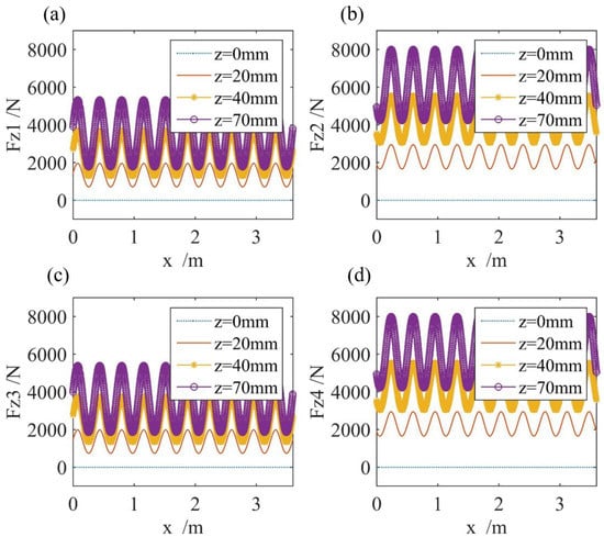
Figure 5. Levitation force on left SCMs when $v=13\hspace{0.33em}\mathrm{mps}$ and $MMF=300\hspace{0.33em}\mathrm{kAt}$: (a) levitation force $F_z^1(x)$; (b) levitation force $F_z^2(x)$; (c) levitation force $F_z^3(x)$; (d) levitation force $F_z^4(x)$.

3. Theory Vertical Equilibrium Point

Because the vehicle is running at a low speed of approximately 14 mps while the MMF is approximately 310 kAt, we sought to discover the location of the theory vertical equilibrium point. Its location is a balance point where the levitation force is equal to gravity, and is useful for designing the initial conditions in multi-body dynamics. The levitation force is decomposed into the oscillation part and average part, which is used to determine the theory vertical equilibrium point, as in Ref. [9].

The levitation force $F_z^i$ is of a periodic quality in Figure 5 and can be divided into the average part $F_{z\_\mathrm{mean}}^i(z)$ and oscillation part $F_{z\_\mathrm{osc}}^i(x,z)$, as shown in Figure 6a,b. Based on the Fourier technique, the levitation force $F_z^i(x,z)$ on the i-th SCM can be decomposed as in Equation (15):

$$F_z^i(x,z)\approx F_{\mathrm{z}\_\mathrm{mean}}^i(z)+F_{\mathrm{z}\_\mathrm{osc}}^i(z,x)\hspace{1em}(i=1,2,3,4)$$

(15)

where $F_{\mathrm{z}\_\mathrm{mean}}^i(z)$ is the average part of the levitation force, and the oscillation part of the levitation force is:

$$F_{\mathrm{z}\_\mathrm{osc}}^i(z,x)={\displaystyle \sum _{n=1}^N{A}_n^i(z)\sin (\frac{2\pi }{Pitch}nx+{\phi }_n^i(z))}$$

(16)

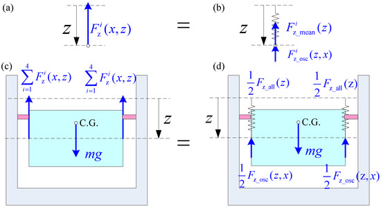
Figure 6. Decomposition of levitation force: (a) i-th levitation force $F_z^i(x,z)$; (b) decomposition of i-th levitation force; (c) force diagram of vehicle with $\gamma (t)=0$; (d) decomposition of force diagram of vehicle with $\gamma (t)=0$.

The average part of the levitation force $F_{\mathrm{z}\_\mathrm{mean}}^i(z)$ in Equation (15) is a non-linear function of $z$ and serves as a non-linear spring force, as shown in Figure 6b. The oscillation part functions as the exciting force.

To decipher the theory vertical equilibrium point, assuming $\gamma (t)=0$, which is according to the calculation of the levitation force, the force diagram of the vehicle in Figure 3c can be simplified as in Figure 6c or Figure 6d. Considering Equation (13), Equation (8) vanishes and Equation (7) should be solved. Substituting Equation (15) into Equation (7), the vertical dynamics equation becomes:

$$m\ddot{z}(t)=mg-{\displaystyle \sum _{i=1}^{4}2F_{\mathrm{z}\_\mathrm{mean}}^i(z)}-{\displaystyle \sum _{i=1}^{4}2}{F}_{\mathrm{z}\_\mathrm{osc}}^i(z,x)$$

(17)

or

$$m\ddot{z}(t)+F_{\mathrm{z}\_\mathrm{all}}^{}(z)=mg-F_{\mathrm{z}\_\mathrm{osc}}^{}(x,z)$$

(18)

where:

$$F_{\mathrm{z}\_\mathrm{all}}(z)={\displaystyle \sum _{i=1}^{4}2F_{\mathrm{z}\_\mathrm{mean}}^i(z)}$$

(19)

$$F_{\mathrm{z}\_\mathrm{osc}}^{}(x,z)=F_{\mathrm{z}\_\mathrm{osc}}^{}(vt,z)={\displaystyle \sum _{i=1}^{4}2}{\displaystyle \sum _{n=1}^N{A}_n^i(z)\sin (\frac{2\pi }{Pitch}nvt+{\phi }_n^i(z))})$$

(20)

The average part of all the levitation forces $F_{\mathrm{z}\_\mathrm{all}}(z)$ depends on z and plays the role of the non-linear spring force. $F_{\mathrm{z}\_\mathrm{osc}}^{}(x,z)$ depends on both z and $x$ functions as the exciting force. When treating the levitation force in the simulation, experts may make $N=1$ to reduce the modelling difficulties in the simulation, as in Ref. [9].

Based on the curve fitting method, $F_{\mathrm{z}\_\mathrm{all}}(z)$ can be fitted by three-order polynomial expression:

$$F_{\mathrm{z}\_\mathrm{all}}(z)=a_1{z}^3+a_2{z}^2+a_{3}z$$

(21)

where $a_1$, $\hspace{0.17em}{a}_2$, and $\hspace{0.17em}{a}_3$ are the fitting parameters. There is no constant term on the right side of Equation (21) as $F_{\mathrm{z}\_\mathrm{all}}(0)=0$.

From Equation (18), the theory vertical equilibrium point $z_0\hspace{1em}(0\hspace{0.33em}\mathrm{mm}<z_0<80\hspace{0.33em}\mathrm{mm})$ satisfies Equation (22):

$$F_{\mathrm{z}\_\mathrm{all}}(z_0)\approx a_1{z}_0^3+a_2{z}_0^2+a_3{z}_0=mg$$

(22)

$F_{\mathrm{z}\_\mathrm{all}}(z)$ nonlinearly depends on z ($z\in [0,2,4,\cdots ,100]\hspace{0.33em}\mathrm{mm}$) and the increment of z is as small as 2 mm, so we may roughly identify the equilibrium point from Figure 7a at different velocities. In fact, we carry out curve fitting through four points, which are the three local points near the equilibrium point $z_0$ and the original point (0, 0) to improve the accuracy. In other words, the fitted curve can traverse the chosen local three points near the equilibrium point and origin point exactly, but the other points are not considered, or it is unnecessary to show the quality of fitting. Figure 7a shows the curve of $F_{\mathrm{z}\_\mathrm{all}}(z)$ when $v\in [13,\hspace{0.17em}\hspace{0.17em}14,\hspace{0.17em}\hspace{0.17em}15]\hspace{0.33em}\mathrm{mps}$ and $MMF=300\hspace{0.33em}\mathrm{kAt}$, and theory vertical equilibrium point $z_0$ is approximately $[43.5,\hspace{0.17em}\hspace{0.17em}41.4,\hspace{0.17em}\hspace{0.17em}39.8]\hspace{0.33em}\mathrm{mm}$, respectively. In other words, the best initial vertical displacement $z(0)=z_0$ is approximately $[43.5,\hspace{0.17em}\hspace{0.17em}41.4,\hspace{0.17em}\hspace{0.17em}39.8]\hspace{0.33em}\mathrm{mm}$ for the small vibration amplitude and the ride stability performance by the vibration theory.

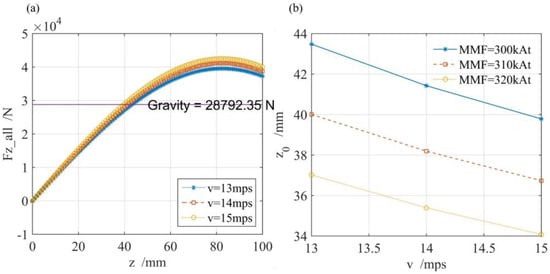
Figure 7. Theory equilibrium point: (a) $F_{\mathrm{z}\_\mathrm{all}}(z)$ when $v\in [13,\hspace{0.17em}\hspace{0.17em}14,\hspace{0.17em}\hspace{0.17em}15]\hspace{0.33em}\mathrm{mps}$ and $MMF=300\hspace{0.33em}\mathrm{kAt}$; (b) theory vertical equilibrium point $z_0$ at $MMF\in [300,310,320]\hspace{0.33em}\mathrm{kAt}$ and $v\in [13,\hspace{0.17em}\hspace{0.17em}14,\hspace{0.17em}\hspace{0.17em}15]\hspace{0.33em}\mathrm{mps}$.

Based on the traversing method, the theory vertical equilibrium point is 34–44 mm, as shown in Figure 7b when $v\in [13,\hspace{0.17em}\hspace{0.17em}14,\hspace{0.17em}\hspace{0.17em}15]\hspace{0.33em}\mathrm{mps}$ and $MMF\in [300,310,320]\hspace{0.33em}\mathrm{kAt}$. Figure 7b shows that when either the $MMF$ or $v$ become larger, the levitation force on each SCM becomes larger and the theory vertical equilibrium point becomes smaller. When testing the dynamic performance of the vehicle, we can roughly achieve $z_0\in [34,44]\hspace{0.33em}\mathrm{mm}$ when $v\in [13,14,15]\hspace{0.33em}\mathrm{mps}$ and $MMF\in [300,310,320]\hspace{0.33em}\mathrm{kAt}$.

4. Multi-Body Dynamic Model of the EDS Vehicle

From Figure 5, the average parts of the levitation forces on the third and fourth SCM are larger than that on the first and second SCM, so the vehicle would pitch. This section shows a new numerical multi-body dynamic model developed to study the vertical displacement and pitch angle in SIMPACK script. The levitation forces are handled by MATLAB/SIMULINK and the tool MATSIM is used to exchange the data.

(1)

Decoupling of Levitation forces

From Section 2.2, when calculating the levitation force, $F_z^i(x,z)$ on the i-th SCM depends on $x$ and $z$ with the constant $v$ and MMF. The levitation forces on the SCMs are coupled with each other through $z$, which is the origin of the body coordinate system $O-XYZ$. To evaluate the pitch angle, this paper decouples the levitation forces from each other. In other words, $F_z^i(x,z)$ is changed to $F_z^i(x,z_i)$, where $z_i$ is the coordinate of i-th SCM.

The levitation force $F_{\mathrm{z}}^i(x,z_i)$ is treated as the exciting force, not decomposed as the right hand of Equation (15). Practically, the levitation force $F_z^i(x,z_i)$ can be interpolated from a 2D matrix $F_z^i(x,z_i)$, where $x=[0,\cdots ,200]\hspace{0.33em}\mathrm{m}$ and $z_i=[0,2,\cdots ,100]\hspace{0.33em}\mathrm{mm}$. For $v\in [13,14,15]\hspace{0.33em}\mathrm{mps}$ and $MMF\in [300,310,320]\hspace{0.33em}\mathrm{kAt}$, a certain levitation force matrix $F_z^i(x,z_i)$ is formed by Equation (23):

$$F_z^i(x,z_i)=\left[\begin{array}{c}{F}_z^i(x)\hspace{1em}for\hspace{1em}{z}_i=0\\ F_z^i(x)\hspace{1em}for\hspace{1em}{z}_i=2\\ ⋮\\ F_z^i(x)\hspace{1em}for\hspace{1em}{z}_i=100\end{array}\right]\hspace{1em}(i=1,2,3,4)$$

(23)

(2)

Model elements in multi-body dynamic model

Figure 8 shows a multi-body dynamic model of the vehicle with six DOF in SIMPACK script. Eight sensor elements obtain the $x$ and $z_i$ values of each SCM in order to decipher the levitation force. Eight control elements (MATSIM) exchange the data between SIMPACK and MATLAB/SIMULINK, which stores the levitation force matrix $F_z^i(x,z_i)$. Eight force elements apply the levitation force value from the control elements to the vehicle. Four contact force elements are used to model the guiding wheels.

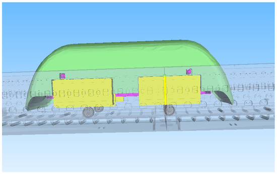
Figure 8. Multi-body co-simulation dynamic model with eight levitation force elements.

(3)

Simulation conditions

Because it is not easy to exactly control the experimental velocity, initial vertical displacement, and MMF, it is better to study the effect of these factors on the dynamic performance of the vehicle to obtain an overall impression. Of course, when all other problems, such as the control system, are solved, an experimental investigation can be carried out. The goal of this paper is to uncover the phenomenon of beat vibration by multi-body dynamics. We assume that the vehicle is running at a steady speed with different initial conditions. Three factors are considered: the initial vertical displacement $z(0)$, velocity $v$, and MMF. The levels of these factors are shown in Table 3. Using the traversing method, considering the influence of these three parameters, the multi-body dynamics model runs $21\times 3\times 3=189$ times.

Table 3. Simulation factors and levels.

Factor	Value	Description
$z(0)$	$[30,31,\cdots ,50]\hspace{0.33em}\mathrm{mm}$	Initial vertical displacement, level number is 21.
$v$	$[13,14,15]\hspace{0.33em}\mathrm{mps}$	Velocity of vehicle, level number is 3.
$MMF$	$[300,310,320]\hspace{0.33em}\mathrm{kAt}$	MMF of SCM onboard, level number is 3.

(4)

Solver setting

The simulation time is 10 s; the sampling rate is 2000 Hz; and the integration method is SODASRT 2.

5. Results and Discussion

5.1. Simulation Results

Figure 9 shows the response of $z(t)$ and $\gamma (t)$ when $v=14\hspace{0.33em}\mathrm{mps}$, $MMF=310\hspace{0.33em}\mathrm{kAt}$, and $z(0)=40\hspace{0.33em}\mathrm{mm}$. The $z(t)$ and $\gamma (t)$ show the phenomenon of beat vibration, which means there are two components with two closing frequencies. Figure 10 shows the $\ddot{z}$ and $\ddot{\gamma }$ response, where the phenomenon of beat vibration exists. The results in Figure 9 and Figure 10 illustrate that the work in this paper successfully predicted the phenomenon of beat vibration. Furthermore, the experimental records in Figure 2 also verify the validity of the dynamic circuit model and mechanical model in this paper.

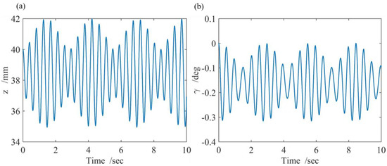
Figure 9. The (a) $z(t)$ and (b) $\gamma (t)$ of the vehicle based on multi-body dynamics when $v=14\hspace{0.33em}\mathrm{mps}$, $MMF=310\hspace{0.33em}\mathrm{kAt}$, and $z(0)=40\hspace{0.33em}\mathrm{mm}$.

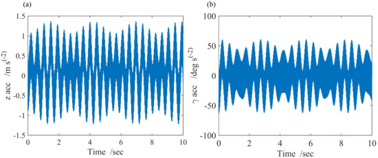
Figure 10. The (a) $\ddot{z}(t)$ and (b) $\ddot{\gamma }(t)$ response based on multi-body dynamics when $v=14\hspace{0.33em}\mathrm{mps}$, $MMF=310\hspace{0.33em}\mathrm{kAt}$, and $z(0)=40\hspace{0.33em}\mathrm{mm}$.

The harmonic exciting frequencies in Equation (16) are $\frac{nv}{Pitch}=\frac{nv}{0.36}\hspace{0.33em}\mathrm{Hz}\hspace{1em}(n=1,2,\cdots ,N)$, i.e., $38.9n\hspace{0.17em}\hspace{0.17em}\mathrm{Hz}$ when $v=14\hspace{0.33em}\mathrm{mps}$. These exciting frequencies are too high to be confirmed only with one’s sense of sight. There are two natural vibration components besides the forced vibration components from the vibration theory. The two natural frequencies of the vehicle are ${\lambda }_1$ and ${\lambda }_2$ because the vertical displacement $z$ and pitch angle $\gamma (t)$ are coupled with each other.

Figure 11 is the FFT transformation of the vertical displacement acceleration $\ddot{z}$ and pitch angle acceleration $\ddot{\gamma }$. The ${\lambda }_1=2\hspace{0.33em}\mathrm{Hz}$ and ${\lambda }_2=2.4\hspace{0.33em}\mathrm{Hz}$ are close to each other and are the two natural frequencies, where $z$ and $\gamma$ are coupled with each other. This is the reason for the phenomenon of beat vibration. The frequencies $38.9\hspace{0.33em}\mathrm{Hz}$ and $77.8\hspace{0.33em}\mathrm{Hz}$ correspond to the first order harmonic exciting frequency $\frac{v}{pitch}=\frac{14}{0.36}\hspace{0.33em}\mathrm{Hz}$ and the second order harmonic exciting frequency $\frac{2v}{pitch}=\frac{2 \times 14}{0.36}\hspace{0.33em}\mathrm{Hz}$ due to the arrangement of figure-eight- shaped coils, respectively. At approximately $38.9\hspace{0.33em}\mathrm{Hz}$ and $77.8\hspace{0.33em}\mathrm{Hz}$, there is a small frequency band where there are local peak frequencies of $[\frac{nv}{pitch}-{\lambda }_2,\frac{nv}{pitch}-{\lambda }_1,\frac{nv}{pitch},\frac{nv}{pitch}+{\lambda }_1,\frac{nv}{pitch}+{\lambda }_2]$ $(n=1,2,\cdots ,N)$. This is due to the amplitude and phase of the n-th harmonic levitation force components $A_n^i(z)$ and ${\phi }_n^i(z)$ $(n=1,2,\cdots ,N)$ depending on $z$ in Equation (16), while $z$ has the harmonic components of the eigenvalues ${\lambda }_1$ and ${\lambda }_2$. If $A_n^i(z)$ and ${\phi }_n^i(z)$ are invariant with $z$ near the equilibrium point, there must be no such small frequency bands near the n-th harmonic exciting frequency $\frac{nv}{pitch}$. The outstanding frequency order of the levitation exciting force is two, as shown in Figure 11. Therefore, it is better to set $N=2$ if experts use the right hand of Equation (15) to obtain a good approximation. This result shows that the method outlined in this paper can provide more detailed dynamic response information of the vehicle than that explored in Section 3.

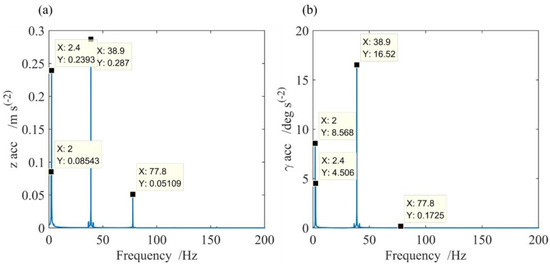
Figure 11. FFT transformation of vertical displacement acceleration and pitch angle acceleration for Figure 10: (a) FFT transformation of $\ddot{z}$; (b) FFT transformation of $\ddot{\gamma }$.

5.2. Vertical Displacement and Pitch Angle Performance under Different Conditions

Based on the traversing method, the vertical displacement $z(t)$ and pitch angle $\gamma (t)$ are calculated by multi-body dynamics 189 times. Four parameters are defined to provide an overview of the vertical movement and pitch angle performance:

(1)

The mean value of the vertical displacement $z_{\mathrm{mean}}$, which indicates that the vertical balance point is defined as:

$$z_{\mathrm{mean}}=\mathrm{mean}(z(t))$$

(24)

(2)

The amplitude of the vertical displacement $z_{\mathrm{amp}}$ is defined as:

$$z_{\mathrm{amp}}=\frac{\max (z(t))-\min (z(t))}{2}$$

(25)

(3)

The mean value of the pitch angle of the vehicle ${\gamma }_{\mathrm{mean}}$, which indicates that the mean pitch angle is defined as:

$${\gamma }_{\mathrm{mean}}=\mathrm{mean}(\gamma (t))$$

(26)

(4)

The amplitude of the pitch angle of the vehicle is defined as ${\gamma }_{\mathrm{amp}:}$

$${\gamma }_{\mathrm{amp}}=\frac{\max (\gamma (t))-\min (\gamma (t))}{2}$$

(27)

$z_{\mathrm{mean}}$, $z_{\mathrm{amp}}$, ${\gamma }_{\mathrm{mean}}$, and ${\gamma }_{\mathrm{amp}}$ for the various initial vertical displacement $z(0)$, velocity $v$, and the $MMF$ of the SCM are plotted in Figure 12, Figure 13 and Figure 14.

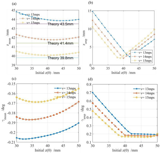
Figure 12. Simulation results when $MMF=300\hspace{0.33em}\mathrm{kAt}$: (a) $z_{\mathrm{mean}}$; (b) $z_{\mathrm{amp}}$ (c) ${\gamma }_{\mathrm{mean}}$; (d) ${\gamma }_{\mathrm{amp}}$.

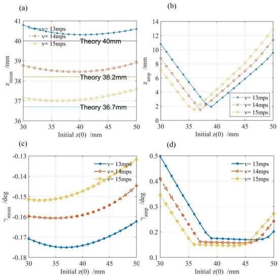
Figure 13. Simulation results when $MMF=310\hspace{0.33em}\mathrm{kAt}$: (a) $z_{\mathrm{mean}}$; (b) $z_{\mathrm{amp}}$ (c) ${\gamma }_{\mathrm{mean}}$; (d) ${\gamma }_{\mathrm{amp}}$.

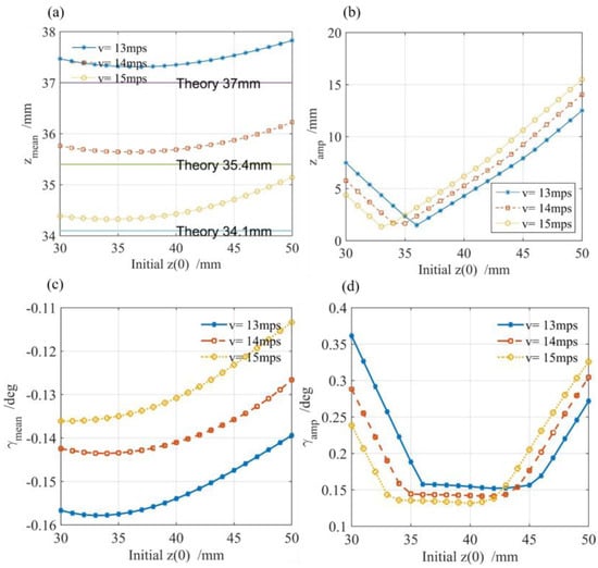
Figure 14. Simulation results when $MMF=320\hspace{0.33em}\mathrm{kAt}$: (a) $z_{\mathrm{mean}}$; (b) $z_{\mathrm{amp}}$; (c) ${\gamma }_{\mathrm{mean}}$; (d) ${\gamma }_{\mathrm{amp}}$.

Because the sum of the levitation forces on the third and fourth SCMs are larger than the sum of that on the first and second SCMs and C.G is on top of the origin of the body system, the negative pitch angle of the vehicle (Figure 12c, Figure 13c and Figure 14c) and the mean value of each $z$ displacement $z_{\mathrm{mean}}$ (Figure 12a, Figure 13a and Figure 14a) are slightly larger than the theory equilibrium point $z_0$ calculated in Section 3. This indicates a good accuracy of the theory equilibrium point.

(1)

Influence of initial vertical displacement $z(0)$

The mean value of the vertical displacement $z_{\mathrm{mean}}$ shows a trend of first decreasing and then increasing as the initial vertical displacement $z(0)$ increases, as shown in Figure 12a, Figure 13a and Figure 14a. The amplitude of the vertical displacement $z_{\mathrm{amp}}$ shows a trend of first decreasing and then increasing as the initial vertical displacement $z(0)$ increases, as shown in Figure 12b, Figure 13b and Figure 14b. Additionally, the vertical displacement becomes larger when $z(0)$ is away from the theory vertical equilibrium point.

The absolute mean value of the pitch angle $\left|{\gamma }_{\mathrm{mean}}\right|$ shows a trend of first increasing and then decreasing as the initial $z(0)$ increases, as shown in Figure 12c, Figure 13c and Figure 14c. The amplitude of the pitch angle ${\gamma }_{\mathrm{amp}}$ shows a trend of first decreasing and then increasing as the initial $z(0)$ increases, as shown in Figure 12d, Figure 13d and Figure 14d.

(2)

Influence of velocity of vehicle $v$

As the velocity $v$ increases, the mean value of the vertical displacement $z_{\mathrm{mean}}$, the amplitude value of the vertical displacement $z_{\mathrm{amp}}$, and the absolute mean value of the vertical displacement of vehicle $\left|{\gamma }_{\mathrm{mean}}\right|$ show a trend of decreasing, as shown in Figure 12a–c to Figure 14a–c.

The amplitude of the pitch angle ${\gamma }_{\mathrm{amp}}$ shows a trend of first decreasing and then increasing as the initial $z(0)$ increases in Figure 12d, Figure 13d and Figure 14d.

(3)

Influence of MMF of SCM

As the MMF of the SCM increases, a decreasing trend is depicted in Figure 12, Figure 13 and Figure 14, which mention the variables of the mean value of the vertical displacement $z_{\mathrm{mean}}$, the amplitude value of the vertical displacement $z_{\mathrm{amp}}$, the absolute mean value of the vertical displacement $\left|{\gamma }_{\mathrm{mean}}\right|$, and the amplitude of the pitch angle ${\gamma }_{\mathrm{amp}}$. This means that an increasing MMF of the SCM is good for vibration control.

6. Conclusions

This paper studied the phenomenon of beat vibration of the HTS EDS of the vehicle at the CRRC. The levitation force on each SCM was calculated based on the dynamic circuit theory with no pitch. (1) The theory vertical equilibrium point was between 34 and 44 mm from the average part of the levitation with no pitch angle when the velocity was 13–15 mps and the MMF was 300–320 kAt. (2) By decoupling the levitation forces from each other, the vertical displacement and pitch angle response from multi-body dynamics successfully showed the phenomenon of beat vibration, which was consistent with the experimental running test. The reason for this was that the two natural frequencies of approximately $2\hspace{0.33em}\mathrm{Hz}$ and $2.4\hspace{0.33em}\mathrm{Hz}$ are close to each other. (3) Considering the influence of the MMF of the SCM, velocity, and initial vertical displacement, the simulation work showed that the higher the velocity or MMF, the smaller the equilibrium point, and the closer the initial vertical displacement is to the theory vertical equilibrium point, the smaller the vibration is. (4) Whether the theory vertical equilibrium point was near the mean equilibrium point was calculated by multi-body dynamics. In this paper, both the numerical results and the experimental phenomenon verified the validity of the dynamic circuit model, the mechanical model, and the method to treat the magnetic force.

References

- Guo, Z.; Zhou, D.; Chen, Q.; Yu, P.; Li, J. Design and Analysis of a Plate Type Electrodynamic Suspension Structure for Ground High Speed Systems. Symmetry 2019, 11, 1117. [Google Scholar] [CrossRef]
- Guo, Z.; Li, J.; Zhou, D. Study of a Null-Flux Coil Electrodynamic Suspension Structure for Evacuated Tube Transportation. Symmetry 2019, 11, 1239. [Google Scholar] [CrossRef]
- Wang, J.S.; Wang, S.Y.; Zeng, Y.W.; Deng, C.Y.; Ren, Z.Y.; Wang, X.R.; Song, H.H.; Zheng, J.; Zhao, Y.; Wang, X.Z. The present status of the high temperature superconducting Maglev vehicle in China. Supercond. Sci. Technol. 2005, 18, S215–S218. [Google Scholar] [CrossRef]
- Bernstein, P.; Noudem, J. Superconducting magnetic levitation: Principle, materials, physics and models. Supercond. Sci. Technol. 2020, 33, 033001. [Google Scholar] [CrossRef]
- Wen, Y.; Xin, Y.; Hong, W.; Zhao, C.; Li, W. Comparative study between electromagnet and permanent magnet rails for HTS maglev. Supercond. Sci. Technol. 2020, 33, 035011. [Google Scholar] [CrossRef]
- Kim, M.; Jeong, J.-H.; Lim, J.; Kim, C.-H.; Won, M. Design and Control of Levitation and Guidance Systems for a Semi-High-Speed Maglev Train. J. Electr. Eng. Technol. 2017, 12, 117–125. [Google Scholar] [CrossRef]
- Powell, J.R.; Danby, G.R. High-Speed Transport by Magnetically Suspended Trains. In Proceedings of the ASME Winter Annual Meeting, 66-WA/RR-5, Railroad Division, New York, NY, USA, 14 November 1966. [Google Scholar]
- Sawada, K. Development of magnetically levitated high speed transport system in Japan. IEEE Trans. Magn. 1996, 32, 2230–2235. [Google Scholar] [CrossRef]
- Ohashi, S.; Ohsaki, H.; Masada, E. Equivalent model of the side wall electrodynamic suspension system. Electr. Eng. Jpn. 1998, 124, 63–73. [Google Scholar] [CrossRef]
- Ohashi, S.; Ohsaki, H.; Masada, E. Effect of the active damper coil system on the lateral displacement of the magnetically levitated bogie. IEEE Trans. Magn. 1999, 35, 4001–4003. [Google Scholar] [CrossRef]
- Takeuchi, T.; Shin, E.; Ohashi, S.; Okubo, T. Improvement of the Damping Factor by the Weight Reduction Damper Coil in Superconducting Magnetically Levitated Bogie. In Proceedings of the 11th International Symposium on Linear Drives for Industry Applications (LDIA), Osaka, Japan, 6–8 September 2017. [Google Scholar]
- Edilson, H.T.; Junior, J.S.; Dynamic Interactions between Maglev Vehicle and Elevated Guideway. SAE Paper 952283. 1995. Available online: https://saemobilus.sae.org/content/952283/ (accessed on 5 December 2022).
- Yan, Z.; Ma, G.; Zhang, W.; Cai, Y.; Zeng, J.; Yao, C.; Song, X.; Jiang, J.; Wang, Y. Dynamic Response of a Superconducting EDS Train with Vehicle/Guideway Coupled Dynamics. IEEE Trans. Appl. Supercond. 2020, 30, 1–5. [Google Scholar] [CrossRef]
- Yan, Z.; Zeng, J.; Zhang, W.; Feng, P.; Li, Y.; Yao, C.; Ma, G. Dynamic Simulation of Vibration Characteristics and Ride Quality of Superconducting EDS Train Considering Body with Flexibility. IEEE Trans. Appl. Supercond. 2021, 31, 1–5. [Google Scholar] [CrossRef]
- Ohashi, S.; Ueda, N. Dependence of the Quenched SC Coil Position on the Transient Motion of the Superconducting Magnetically Levitated Bogie. IEEE Trans. Appl. Supercond. 2016, 26, 1–4. [Google Scholar] [CrossRef]
- Ohashi, S.; Ohsaki, H.; Masada, E. Running Characteristics of the superconducting magnetically levitated train in the case of superconducting coil quenching. Electr. Eng. Jpn. 2000, 130, 937–946. [Google Scholar] [CrossRef]
- Seino, H.; Miyamoto, S. Long-term Durability and Special Running Tests on the Yamanashi Maglev Test Line. Q. Rep. RTRI 2006, 47, 1–5. [Google Scholar] [CrossRef]
- Chen, D.; Li, X.-F.; Wu, W.; Sheng, J.; Hong, Z.; Jin, Z.; Ma, H.; Zhao, T. A Three-dimensional Numerical Model for Evaluation of Eddy Current Effects on Electromagnetic Forces of HTS Electrodynamic Suspension System. Phys. C Supercond. Appl. 2022, 594, 1354009. [Google Scholar] [CrossRef]
- Chen, D.; Li, X.-F.; Huang, X.; Sheng, J.; Wu, W.; Hong, Z.; Jin, Z.; Ma, H.; Zhao, T. An FEM Model for Evaluation of Force Performance of High-Temperature Superconducting Null-Flux Electrodynamic Maglev System. IEEE Trans. Appl. Supercond. 2021, 31, 3603806. [Google Scholar] [CrossRef]
Disclaimer/Publisher’s Note: The statements, opinions and data contained in all publications are solely those of the individual author(s) and contributor(s) and not of MDPI and/or the editor(s). MDPI and/or the editor(s) disclaim responsibility for any injury to people or property resulting from any ideas, methods, instructions or products referred to in the content. |
© 2023 by the authors. Licensee MDPI, Basel, Switzerland. This article is an open access article distributed under the terms and conditions of the Creative Commons Attribution (CC BY) license (https://creativecommons.org/licenses/by/4.0/).