Optimization of BP Neural Network Model for Rockburst Prediction under Multiple Influence Factors

Abstract

Rockbursts are serious threats to the safe production of mining, resulting in great casualties and property losses. The accurate prediction of rockburst is an important premise that influences the safety and health of miners. As a classical machine learning algorithm, the back propagation (BP) neural network has been widely used in rockburst prediction. However, there are few reports about the influence study of different training sample sizes, optimization algorithms and index dimensionless methods on the prediction accuracy of BP neural network models. Therefore, 100 groups of typical rockburst engineering samples were collected locally and abroad, and considering the relevance, scientificity and quantifiability of the prediction indexes, the ratio of the maximum tangential stress of surrounding rock to the rock uniaxial compressive strength (σ_θ/σ_c), the ratio of the rock uniaxial compressive strength to the rock uniaxial tensile strength (σ_c/σ_t) and the elastic energy index (W_et) were chosen as the prediction indexes. When the number of samples was 40, 70 and 100, sixty improved BP models were established based on the standard gradient descent algorithm and four optimization algorithms (momentum gradient descent algorithm, quasi-Newton algorithm, conjugate gradient algorithm, Levenberg–Marquardt algorithm) and four index dimensionless methods (unified extreme value processing method, differentiated extreme value processing method, data averaging processing method, normalized processing method). The prediction performances of each improved model were compared with those of standard BP models. The comparative study results indicate that the sample size, optimization algorithm and dimensionless method have different effects on the prediction accuracy of BP models, which are described as follows: (1) The prediction accuracy value A of the BP model increases with the addition of sample size. The average value A_ave of twenty improved models under three kinds of sample sizes increases from A_ave (40) = 69.7% to A_ave (100) = 75.3%, with a maximal value A_max from A_max (40) = 85.0% to A_max (100) = 97.0%. (2) The value A and comprehensive accuracy value C of the BP model based on four optimization algorithms are generally higher than those of the standard BP model. (3) The improved BP model based on the unified extreme value processing method combined with the Levenberg–Marquardt algorithm has the highest value A_max (100) = 97.0% and value C = 194, and the prediction results of five engineering cases are completely consistent with the actual situation at the site, so this is the best BP neural network model selected in this paper.

1. Introduction

Construction activities (drilling and blasting) of large underground caverns and tunnel excavations, etc., inevitably cause internal damage and redistribution of in situ stress rock masses, which are easy to induce brittle failures, such as spalling, cracking and rockburst [1,2]. Rockburst is a phenomenon in which the elastic energy gathered in a rock mass is released suddenly and violently under external influence, resulting in rockbursting or ejection. In 1900, rockburst was first observed in the Kolar gold mine of India, which has frequently occurred in the construction of mines, hydraulic works, tunnels and other projects in many countries [3,4,5,6].

The prediction and evaluation of rockburst are important prerequisites for formulating prevention and control measures. In recent years, machine learning techniques have been applied well in the field of classification and recognition, and they have become promising methods in rockburst prediction, such as support vector machine [7,8], neural network [9,10], random forest [11,12], cloud model [13,14], extreme learning machine [15,16], Bayesian classifier [17,18], decision tree [19,20], fuzzy C-means clustering [21] and logistic regression model [22]. As a classical supervised learning algorithm, the BP (ack propagation) neural network has been widely used in rockburst prediction [23,24,25]. Most of the existing studies used a standard BP neural network, that is, using a gradient descent algorithm to train the model, which has some disadvantages, including sensitive initial weight setting, local extreme value prone to occur, slow convergence speed, difficult selection of network structure, etc. Given these deficiencies, Li et al. [26] used Levenberg–Marquardt algorithm to train a BP network and improve the efficiency of the standard model. Wang [27] optimized the network by adding linear transfer functions, momentum terms and introducing a new training method (Resilient BP). Sun [28] adjusted the weight and threshold of the algorithm structure by increasing the self-adaptability and momentum term coefficient. Zhang et al. [29] used particle swarm optimization, and Hu et al. [30] used a genetic algorithm to optimize the initial weights and thresholds of a BP network, which improved the prediction accuracy of the model. Meng et al. [31] established an improved BP neural network adopting an adaptive learning rate algorithm and an algorithm based on numerical optimization technology. Existing studies have used different optimization algorithms to improve the standard BP network model and achieved good results. However, a comparative analysis of optimization effects among multiple different algorithms has not been carried out, and the influence of different index dimensionless methods on the prediction accuracy of the BP model has not been discussed.

Therefore, based on three sample sizes of rockburst examples (40, 70 and 100), this paper selects a standard gradient descent algorithm, four typical optimization algorithms (momentum gradient descent algorithm, quasi-Newton algorithm, conjugate gradient algorithm and Levenberg–Marquardt algorithm) and four commonly used index dimensionless methods (unified extreme value processing method, differentiated extreme value processing method, data averaging processing method and normalization processing method). Additionally, it establishes sixty BP prediction models, systematically carries out comparative research on model prediction effect, optimizes the best rockburst prediction model and applies it to engineering cases.

This manuscript is an extension of the conference paper BP neural network model optimization for rockburst prediction considering sample sizes, optimization algorithms and dimensionless methods. No copyright issue is involved.

2. Principle

2.1. Dimensionless Methods

Dimensionless methods are commonly used data normalization methods. Due to the different dimensions of indexes, they are not comparable. Therefore, the indexes should be processed by the dimensionless method first and then analyzed after eliminating the dimensional influence. In this paper, we selected four dimensionless methods (unified extreme value processing method, differentiated extreme value processing method, data averaging processing method and normalized processing method) to process the original index data.

(1)

Unified extreme value processing method

The principle of the unified extreme value processing method is shown in Equation (1):

$${x_{ij}}^{\ast }=\frac{x_{ij}-\min (x_j)}{\max (x_j)-\min (x_j)}(i=1,2,\dots ,m;j=1,2,\dots ,n)$$

(1)

where x_ij is the original data of the j-th index of the i-th sample; x_ij^* is the data after processing, where the value is between 0 and 1, and the value distribution is consistent with that before processing; max(x_j) and min(x_j) are the maximum and minimum values of the original data of the j-th index, respectively.

(2)

Differentiated extreme value processing method

The unified extreme value processing method adopts a unified formula for the forward index (that is, the larger the data, the more dangerous the rockburst, such as σ_θ/σ_c and W_et) and reverse index (that is, the smaller the data, the more dangerous the rockburst, such as σ_c/σ_t). However, the indexes are processed differently by the differentiated extreme value processing method, as shown in Equation (2) for the forward index and Equation (3) for the reverse index:

$${x_{ij}}^{\ast }=\frac{x_{ij}-\min (x_j)}{\max (x_j)-\min (x_j)}$$

(2)

$${x_{ij}}^{\ast }=\frac{\max (x_j)-x_{ij}}{\max (x_j)-\min (x_j)}$$

(3)

(3)

Data averaging processing method

The principle of the data-averaging processing method is shown in Equation (4):

$${x_{ij}}^{\ast }=\frac{x_{ij}}{\overline{x}}$$

(4)

where $\overline{x}$ is the average value of the original samples data of the j-th index.

This method maintains the overall consistency of the original data well while eliminating the effects of dimension and order of magnitude, which retains the information of the original variation degree of each index.

(4)

Normalized processing method

The principle of the normalized processing method is shown in Equation (5):

$${x_{ij}}^{\ast }=\frac{x_{ij}}{{\displaystyle \sum _{i=1}^m{x}_{ij}}}$$

(5)

This method converts the actual value of the index into its proportion in the total value of the index, so it is also called the proportion method.

2.2. BP Neural Network

The BP neural network is a multilayer feed-forward network based on the BP algorithm. The network has the advantages of self-learning and self-adaptation, where the structure is simple, and the algorithm is mature. The standard BP neural network is usually composed of an input layer, hidden layer and output layer. The input layer of the BP neural network constructed in this paper has three neurons, which are the dimensionless values of σ_θ/σ_c, σ_c/σ_t and W_et. This paper set two hidden layers that, after extensive debugging, have node numbers 10 and 4, respectively. There are four neurons in the output layer, corresponding to rockburst risk levels I–IV to which the samples belong, as shown in Figure 1.

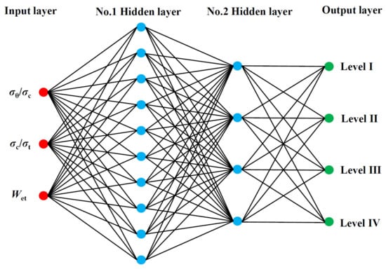
Figure 1. Structure of the BP neural network.

The standard BP neural network uses a gradient descent algorithm to train the network and adjust the error. In order to optimize the BP neural network model, four unconstrained optimization algorithms (momentum gradient descent algorithm, quasi–Newton algorithm, conjugate gradient algorithm and Levenberg–Marquardt algorithm) are used to train the network. These five algorithms can be called by the corresponding training function in the MATLAB neural network toolbox.

3. Index Selection and Data Analysis

The mechanism of rockburst is complex, and its causes are numerous. Considering the internal cause (physical and mechanical properties of the rock itself) and the external cause (e.g., stress concentration caused by excavation), this paper selected the ratio of maximum tangential stress of surrounding rock to rock uniaxial compressive strength (σ_θ/σ_c), the ratio of rock uniaxial compressive strength to rock uniaxial tensile strength (σ_c/σ_t) and the elastic energy index (W_et) [32] as prediction indexes. The reasons for selecting these indexes are as follows: σ_θ/σ_c–this index considers the adjustment and change in stress after excavation of underground space and the stress concentration phenomenon of surrounding rock, which reflects the potential influence of the stress state of surrounding rock on the surrounding rock, and reflects the stress condition background of rockburst. The σ_c/σ_t index is the strength brittleness coefficient, which refers to the dynamic process of rockburst. The rock mass undergoes brittle fracture, and the surrounding rock also produces unstable failure, so the degree of brittle failure is closely related to rock eruption. W_et is the elastic energy index that describes the conditions of rock eruption from the perspective of energy; its value reflects the energy storage characteristics of the rock mass, and the higher the rockburst, the more energy is released when a rockburst occurs. The intensity of the rockburst is graded into four levels: level I (none rockburst), level II(weak rockburst), level III (moderate rockburst) and level IV (strong rockburst).

In this paper, 100 groups of rockburst samples were extensively collected from around the world [33,34,35,36], including 19 level I samples, 27 level II samples, 36 level III samples and 18 level IV samples. The full sample data can be found in Appendix A “Sample data”. Figure 2 shows the boxplot of the rockburst prediction indexes, which shows the mean value; the upper and lower bounds of the 95% confidence interval for the mean value; the median; the variance; the standard deviation; and the maximum value for the rockburst prediction index, minimum value, range, interquartile range, skewness and kurtosis, and some characteristic values are shown in Table 1.

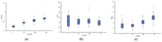
Figure 2. Box plot of prediction indexes: (a) σ_θ/σ_c; (b) σ_c/σ_t; (c) W_et.

Table 1. Statistical parameters of rockburst prediction indexes.

Level	Characteristic	σθ/σc	σc/σt	Wet
I	mean	0.20	24.49	2.99
	median	0.20	23.00	2.00
	minimum	0.10	6.70	1.40
	maximum	0.43	47.90	7.40
	standard deviation	0.20	36.00	2.30
II	mean	0.43	20.77	2.94
	median	0.42	20.40	2.90
	minimum	0.22	6.80	0.90
	maximum	0.67	34.30	5.10
	standard deviation	0.37	24.00	5.10
III	mean	0.57	24.20	4.41
	median	0.56	21.85	4.30
	minimum	0.28	9.50	2.00
	maximum	0.84	55.00	7.10
	standard deviation	0.40	14.70	7.10
IV	mean	0.72	19.08	6.18
	median	0.68	17.25	6.25
	minimum	0.42	11.20	2.00
	maximum	1.41	32.20	10.90
	standard deviation	0.58	13.20	6.30

4. Research Method

The collected rockburst samples were divided into three different sizes (40, 70 and 100), among which the proportion of samples in the training set and test set was 7:3. Four dimensionless methods were selected to process the prediction indexes, and the processed data were used as the input layer of the BP neural network for training and testing. The gradient descent algorithm and four optimization algorithms were used to construct training functions, and different BP neural network models were established. Under different sample sizes, the 1#–3# optimal models were selected initially, and then the best optimal model was finally selected from the three optimal models for engineering applications. Figure 3 shows the flow chart of model optimization.

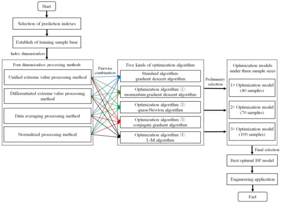
Figure 3. Flow chart of model optimization.

5. Prediction Results and Analysis

5.1. Prediction Results

This paper defines the prediction accuracy rate A to compare and analyzes the prediction effects of different models. A represents the ratio of the correctly predicted sample number to the total sample number, as shown in Equation (6). The higher the A value is, the better the predicted effect of the model.

$$A=\frac{N_{\mathrm{train}}^{\prime }+N_{test}^{\prime }}{N_{train}+N_{test}}$$

(6)

where $N_{train}$ and $N_{test}$ are the sample numbers of the training set and test set, respectively, and $N_{\mathrm{train}}^{\prime }$ and $N_{test}^{\prime }$ are the correctly predicted sample numbers of the training set and test set, respectively.

In the case of sample sizes of 40, 70 and 100, based on four index dimensionless methods and five algorithms (gradient descent algorithm and four optimization algorithms), sixty BP models are established, including the standard BP neural network model based on the gradient descent algorithm (standard BP model), BP neural network optimization model based on the momentum gradient descent algorithm (GDM–BP model), BP neural network optimization model based on the quasi–Newton algorithm (BFG–BP model), BP neural network optimization model based on the conjugate gradient algorithm (SCG–BP model) and BP neural network optimization model based on the Levenberg–Marquardt algorithm (LM–BP model) [37]. There are twenty BP models under each sample size, and their prediction accuracy rate A is shown in Table 2. Figure 4 shows the accuracy rate A of the model under different dimensionless methods.

Table 2. Prediction results of the BP model.

Prediction Model	Index Dimensionless Method	A (40)/%	A (70)/%	A (100)/%
Standard BP model	Unified extreme value processing method	70.0	60.0	75.0
	Differential extreme value processing method	77.5	48.6	59.0
	Normalized processing method	67.5	67.1	60.0
	Data averaging processing method	70.0	52.9	68.0
GDM–BP model	Unified extreme value processing method	62.5	57.1	69.0
	Differential extreme value processing method	52.5	60.0	69.0
	Normalized processing method	67.5	54.3	62.0
	Data averaging processing method	67.5	57.1	66.0
BFG–BP model	Unified extreme value processing method	72.5	70.0	89.0
	Differential extreme value processing method	65.0	70.0	81.0
	Normalized processing method	65.0	88.6	64.0
	Data averaging processing method	85.0	65.7	91.0
SCG–BP model	Unified extreme value processing method	80.0	82.9	95.0
	Differential extreme value processing method	77.5	81.4	78.0
	Normalized processing method	60.0	70.0	45.0
	Data averaging processing method	65.0	70.0	91.0
LM–BP model	Unified extreme value processing method	80.0	92.9	97.0
	Differential extreme value processing method	72.5	88.6	94.0
	Normalized processing method	70.0	84.3	58.0
	Data averaging processing method	67.5	92.9	95.0

Note: A (40), A (70) and A (100) refer to the prediction accuracy of the BP model when the sample size is 40, 70 and 100, respectively.

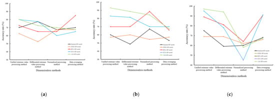
Figure 4. Model accuracy rate A under different dimensionless methods: (a) sample size 40; (b) sample size 70; (c) sample size 100.

5.2. Analysis

To better measure the prediction accuracy of the model, considering the influence of different sample sizes, the prediction results of multiple modeling with different sample numbers of the same model were integrated, and the comprehensive, accurate value C, which reflects the prediction accuracy of different models under the same conditions, was used for comparison, as shown in Equation (7).

$$C={\displaystyle \sum _{i=1}^n{C}_i}$$

(7)

where C_i is the number of accurate samples predicted by the model, i-th is the sample size and n is the number of types of sample size; in this paper, n = 3 (as 40,70 and 100).

The larger the C value is, the higher the accuracy and the better the prediction effect. Table 3 shows the comprehensive, accurate values of different models.

Table 3. Comprehensive, accurate values C of different models.

Prediction Model	Unified Extreme Value Processing Method	Differentiated Extreme Value Processing Method	Normalized Processing Method	Data Averaging Processing Method
Standard BP model	145	124	134	133
GDM–BP model	134	132	127	133
BFG–BP model	167	156	152	171
SCG–BP model	185	166	118	166
LM–BP model	194	185	145	187

Table 3 shows that the dimensionless method has different influences on the predicted effect of the BP model, and the influence degree can be directly reflected by the extreme difference in the comprehensive accuracy value C. The larger the extreme difference value is, the greater the difference in the prediction results of the model with the dimensionless method. Therefore, the extreme difference value of C can be used to measure the prediction stability of a BP neural network model. Because the smaller the range of the extreme difference value of C is, the closer the model prediction result is, different dimensionless methods have less influence on the BP neural network model. Prediction stability is the excellent performance of a model. The prediction stability of a model is good, which indicates that the data requirement of the model itself can be reduced. In other words, if the prediction stability of the model is good, it is unnecessary to use specific methods to process data. Of course, all of these are based on a small difference in forecast accuracy. Table 4 shows the extreme difference values of C for different dimensionless methods under the same model.

Table 4. Extreme difference values of C for different dimensionless methods under the same model.

Prediction Model	Extreme Difference
Standard BP model	21
GDM–BP model	7
BFG–BP model	19
SCG–BP model	67
LM–BP model	49

As seen from Table 4, dimensionless methods have the greatest impact on the SCG–BP model and the least impact on the GDM–BP model. The results show that the GDM-BP model has the minimum requirements for the dimensionless method, and the prediction accuracy differs little when different dimensionless methods are adopted and vice versa for the SCG-BP model.

Similarly, the extreme difference values of C for different prediction models under the same dimensionless method can be calculated, as shown in Table 5.

Table 5. Extreme difference values of C for different prediction models under the same dimensionless method.

Dimensionless Method	Extreme Difference
Unified extreme value processing	60
Differentiated extreme value processing	51
Normalized processing	34
Data averaging processing	54

According to Table 4 and Table 5, compared with the impact of the dimensionless method on the prediction model, the selection of BP neural network models has a more significant impact on the prediction results.

From the above analysis, it is clear that both the dimensionless method and the model training method are important factors affecting the prediction effect of the model. Therefore, the model prediction accuracy P_a and the prediction stability P_s are considered in this paper for model optimization. P_a is measured by the comprehensive, accurate value C and A_max (the prediction accuracy under the maximum sample size), where the C reflects the comprehensive prediction performance of the model under different sample sizes, the A_max reflects the prediction effect when the size of samples is the largest, and the combination of the two can ensure the prediction accuracy effectiveness. The prediction stability P_s is measured by the C’s extreme difference. For model preference, prediction accuracy P_a is considered first, and prediction stability P_s can be used as an auxiliary discriminant factor. If the model prediction accuracy varies greatly, the influence of stability can be ignored. When the difference between the two models’ C values is less than or equal to 5, the model with better prediction stability is preferred in this paper.

Based on the above analysis, the predicted effect of the LM–BP neural network based on the unified extreme value processing method is best among the sixty prediction models, and its A_max (100) = 97.0% and C = 194, both of which are maximum values. Therefore, the LM-BP model is the best optimal model in this paper.

In order to study the influence of sample size on the prediction effect of the BP neural network model, the average and maximum prediction accuracy rates of twenty BP models under different sample sizes were calculated, as shown in Figure 5. It can be seen that with the increase in sample size, the average and maximum prediction accuracy rates both increase nonlinearly. Therefore, the expansion of the sample size is one of the conditions for improving the prediction accuracy of the BP model.

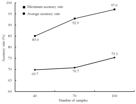
Figure 5. Model accuracy rate under different sample sizes.

5.3. Limitation

In this paper, the BP neural network model was used to study rockburst prediction, and a series of conclusions were obtained, but there are still some shortcomings. The research conclusions of this paper are only applicable to the BP neural network under the database of this paper, and similar conclusions may not be possible for other models. In addition, the sample library established in this paper is small and unbalanced, which may have a certain impact on the prediction results. As can be seen from Figure 2, there are fewer outliers in the data, but different levels of the same indicator are different, and the existing feature optimization studies are based on overall optimization [38,39]. For local optimization implementations, this may have an impact on the results.

6. Engineering Application

To verify the engineering application effect of the best optimal model, the LM–BP neural network model based on the unified extreme value processing method to process data was applied to five engineering cases, namely, the Maluping mine (case 1) [40], the −730 level of Dongguashan copper mine (case 2) [41], the 3 + 390 working face of Jinping II hydropower station (case 3) [41], the Qinling tunnel (case 4) [41] and the highway tunnel of Zhongnan mountain (case 5) [42]. Rockburst occurred in these projects, and the values of σ_θ/σ_c, σ_c/σ_t, and W_et are all worth recording. The prediction results are compared with those of the support vector machine (SVM) model and decision tree based on the same training samples.

(1)

Maluping mine

The Maluping mine area of the Kailin group is located in the northern section of the east flank of Yangshui Anticline, with a stratigraphic inclination of 110°–165° and a typical dip angle of 20°–35°. Additionally, the structure is dominated by faults, all of which are strike faults. The LM-BP neural network model is applied to predict the rockburst in the mining area with a 750 m middle section and red shale lithology. The prediction results are consistent with the SVM model, as shown in Table 6. The field records show that the roadway at this place has produced a sidewall and weak rockburst. The prediction results in this paper are consistent with the field situation [40].

Table 6. Rockburst data and prediction results of Maluping mine.

No.	Prediction Indexes			Actual Level	Prediction Results
	σθ/σc	σc/σt	Wet		LM-BP Model	Decision Tree	SVM Model
1	0.45	11.20	2.03	II	II	II	II

(2)

Dongguashan copper mine

Dongguashan copper mine is the first typical deep-buried hard rock metal mine with rockburst proneness in China. Its main ore body is located at −680 m–1000 m, most of which are located below −730 m above sea level. The maximum principal stress of the ore body is 30–38 MPa, which belongs to a high-stress region, and rockburst occur many times during the mining process. The LM-BP neural network model is used to predict the rockburst of the Dongguashan copper mine. The prediction results are consistent with the DA-DNN model (based on the dropout and the improved Adam’s deep neural network) and the cloud model, as shown in Table 7. There was a rockburst in the skarn at −790 m in this mine. After supporting by an anchor net, the anchor rod was cut off, and a 1.8 m long floor heave appeared at the boundary of the strata [41]. It can be seen that the prediction results in this paper are consistent with the field conditions and are better than the SVM model (misjudged case 2 from level III to level II).

Table 7. Rockburst data and prediction results of Dongguashan mine.

No.	Prediction Indexes			Actual Level	Prediction Results
	σθ/σc	σc/σt	Wet		LM-BP Model	Decision Tree	SVM Model	DA-DNN Model [41]	Cloud Model [41]
2	0.46	11.10	3.97	III	III	II	II	III	III

(3)

3 + 390 working face of Jinping II hydropower station

Jinping II hydropower station is located in a high-stress area of southwest China. The buried depth of a water diversion tunnel is generally 1500–2000 m, and the maximum buried depth is 2525 m. The tunnel rock mass is relatively complete, and the uniaxial compressive strength of the rock is 55–114 MPa, with the maximum major principal stress of 46 MPa measured. The rockburst phenomena have occurred several times since the tunnel construction. The LM-BP neural network model is used to predict rockburst on the 3 + 390 working face of the Jinping II hydropower station. The prediction results are consistent with the SVM model, cloud model and the actual situation, as shown in Table 8.

Table 8. Rockburst data and prediction results of Jinping II hydropower station.

No.	Prediction Indexes			Actual Level	Prediction Results
	σθ/σc	σc/σt	Wet		LM-BP Model	Decision Tree	SVM Model	Cloud Model [42]
3	0.84	19.69	2.30	III	III	III	III	III

In this paper, the rockburst prediction results of the Qinling tunnel (case 4) and the highway tunnel of Zhongnan mountain (case 5) by the LM-BP neural network model is as shown in Table 9. The prediction results are completely consistent with the actual engineering situation, while the SVM model predicts case 4 from level III to level IV.

Table 9. Prediction results of 4^# and 5^# cases.

No.	Prediction Indexes			Actual Level	Prediction Results
	σθ/σc	σc/σt	Wet		LM-BP Model	Decision Tree	SVM Model
4	0.42	13.98	7.44	III	III	IV	IV
5	0.65	28.60	6.80	IV	IV	IV	IV

Based on the prediction results of the above five engineering cases, the prediction results of the LM–BP model are completely consistent with the situation in the field. However, the SVM model misjudged case 2 from level III to II and case 4 from level III to IV, as shown in Figure 6.

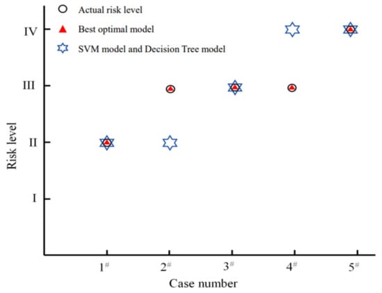
Figure 6. Comparison of prediction results.

7. Conclusions

The present paper selected the ratio of the maximum tangential stress of surrounding rock to the rock uniaxial compressive strength (σ_θ/σ_c), the ratio of the rock uniaxial compressive strength to the rock uniaxial tensile strength (σ_c/σ_t) and the elastic energy index (W_et) as prediction indexes, and extensively collected 100 groups of typical rockburst samples. Based on standard algorithms, four optimization algorithms and four index dimensionless methods, this paper established sixty BP models in total for rockburst prediction with sample sizes of 40, 70 and 100. The following conclusions can be drawn:

(1) Comparative study and engineering application results show that the LM–BP neural network based on the unified extreme processing method has the best prediction effect, which is the best optimal model.

(2) The selection of dimensionless methods has different influences on the prediction results of the BP neural network model, the SCG–BP model has the greatest influence and the GDM–BP model has the least influence. Compared with the dimensionless method, the selection of the training function of the BP neural network has a more significant influence on the prediction results.

(3) With the addition of training samples, the average and maximum prediction accuracy rates of the BP model both increase nonlinearly. Therefore, it is necessary to increase the number of typical rockburst samples and gradually improve the prediction accuracy of the BP model in the future.

References

- Zhao, J.; Jiang, Q.; Lu, J.F.; Chen, B.R.; Pei, S.F.; Wang, Z.L. Rock fracturing observation based on microseismic monitoring and borehole imaging: In situ investigation in a large underground cavern under high geo-stress. Tunn. Undergr. Space Technol. 2022, 126, 104549. [Google Scholar] [CrossRef]
- Zhao, J.; Jiang, Q.; Pei, S.; Chen, B.; Xu, D.P.; Song, L.B. Microseismicity and focal mechanism of blasting-induced block falling of intersecting chamber of large underground cavern under high geostress. J. Cent. South Univ. 2023, 30. [Google Scholar] [CrossRef]
- Du, W. Research on the law of geological disasters and prevention and control measures of tunnel excavation. D. Cent. South Univ. 2001.
- Adoko, A.; Gokceoglu, C.; Wu, L.; Zuo, Q. Knowledge-based and data-driven fuzzy modeling for rockburst prediction. Int. J. Rock Mech. Min. Sci. 2013, 61, 86–95. [Google Scholar] [CrossRef]
- Li, Y.; Wang, C.; Xu, J.; Zhou, Z.; Xu, J.; Cheng, J. Rockburst prediction based on the KPCA-APSO-SVM model and its engineering application. Shock. Vib. 2021, 2021, 7968730. [Google Scholar] [CrossRef]
- Li, X.; Eunhye, K.; Gabriel, W. A study of rock pillar behaviors in laboratory and in-situ scales using combined finite-discrete element method models. Int. J. Rock Mech. Min. Sci. 2019, 118, 21–32. [Google Scholar] [CrossRef]
- Zhou, J.; Li, X.; Shi, X. Long-term prediction model of rockburst in underground openings using heuristic algorithms and support vector machines. Saf. Sci. 2012, 50, 629–644. [Google Scholar] [CrossRef]
- Pu, Y.; Apel, D.; Xu, H. Rockburst prediction in kimberlite with unsupervised learning method and support vector classifier. Tunn. Undergr. Space Technol. 2019, 90, 12–18. [Google Scholar] [CrossRef]
- Faradonbeh, R.; Taheri, A. Long-term prediction of rockburst hazard in deep underground openings using three robust data mining techniques. Eng. Comput. 2019, 35, 659–675. [Google Scholar] [CrossRef]
- Yin, X.; Liu, Q.; Pan, Y.; Huang, X.; Wu, J.; Wang, X. Strength of stacking technique of ensemble learning in rockburst prediction with imbalanced data: Comparison of eight single and ensemble models. Nat. Resour. Res. 2021, 30, 1795–1815. [Google Scholar] [CrossRef]
- Dong, L.; Li, X.; Peng, K. Prediction of rockburst classification using random forest. Trans. Nonferrous. Met. Soc. China 2013, 23, 472–477. [Google Scholar] [CrossRef]
- Liang, W.; Sari, A.; Zhao, G.; McKinnon, D.; Wu, H. Short-term rockburst risk prediction using ensemble learning methods. Nat. Hazards 2020, 104, 1923–1946. [Google Scholar] [CrossRef]
- Liu, J.; Shi, H.; Wang, R.; Si, Y.; Wei, D.; Wang, Y. Quantitative risk assessment for deep tunnel failure based on normal cloud model: A case study at the Ashele copper mine, China. Appl. Sci. 2021, 11, 5208. [Google Scholar] [CrossRef]
- Lin, Y.; Zhou, K.; Li, J. Application of cloud model in rockburst prediction and performance comparison with three machine learning algorithms. IEEE Access 2018, 6, 2839754. [Google Scholar]
- Li, T.; Li, Y.; Yang, X. Rockburst prediction based on genetic algorithms and extreme learning machine. J. Cent. South Univ. 2017, 24, 2105–2113. [Google Scholar] [CrossRef]
- Xue, Y.; Bai, C.; Qiu, D.; Kong, F.; Li, Z. Predicting rockburst with database using particle swarm optimization and extreme learning machine. Tunn. Undergr. Space Technol. 2020, 98, 103287. [Google Scholar] [CrossRef]
- Sousa, L.; Miranda, T.; Sousa, R.; Tinoco, J. The use of data mining techniques in rockburst risk assessment. Engineering 2017, 3, 552–558. [Google Scholar] [CrossRef]
- Li, N.; Feng, X.; Jimenez, R. Predicting rockburst hazard with incomplete data using Bayesian networks. Tunn. Undergr. Space Technol. 2017, 61, 61–70. [Google Scholar] [CrossRef]
- Pu, Y.; Apel, D.; Lingga, B. Rockburst prediction in kimberlite using decision tree with incomplete data. J. Sustain. Min. 2018, 17, 158–165. [Google Scholar] [CrossRef]
- Ghasemi, E.; Gholizadeh, H.; Adoko, A. Evaluation of rockburst occurrence and intensity in underground structures using decision tree approach. Eng. Comput. 2020, 36, 213–225. [Google Scholar] [CrossRef]
- Faradonbeh, R.; Haghshenas, S.; Taheri, A.; Mikaeil, R. Application of self-organizing map and fuzzy c-mean techniques for rockburst clustering in deep underground projects. Neural Comput. Appl. 2019, 32, 8545–8559. [Google Scholar] [CrossRef]
- Afraei, S.; Shahriar, K.; Madani, H. Statistical assessment of rockburst potential and contributions of considered predictor variables in the task. Tunn. Undergr. Space Technol. 2018, 72, 250–271. [Google Scholar] [CrossRef]
- Ding, X.; Wu, J.; Li, J.; Liu, C. Artificial neural network for forecasting and classification of rockbursts. J. Hohai Univ. Nat. Sci. 2003, 31, 424–427. [Google Scholar]
- Guo, L.; Wu, A.; Ma, D. The method to predict rockbursts proneness based on RES theory. J. Cent. South Univ. Nat. Sci. 2004, 35, 304–309. [Google Scholar] [CrossRef]
- Bai, M.; Wang, L.; Xu, Z. Study on a neutral network model and its application in predicting the risk of rock blast. China Saf. Sci. J. 2002, 12, 65–69. [Google Scholar]
- Li, Y.; Yin, J.; Ai, K. Application of BP neural network in prediction of rockburst. J. Yangtze River Sci. Res. Inst. 2008, 25, 183–185+190. [Google Scholar] [CrossRef]
- Wang, B. Application of improved BP neural network in tunnel rockburst prediction. Transp. Stand 2010, 29, 86–89. [Google Scholar]
- Sun, C. A prediction model of rockburst in tunnel based on the improved MATLAB-BP neural network. J. Chongqing Jiaotong Univ. Nat. Sci. 2019, 38, 41–49. [Google Scholar]
- Zhang, Q.; Wang, W.; Liu, T. Prediction of rockbursts based on particle swarm optimization-BP neural network. J. China Three Gorges Univ. Nat. Sci. 2011, 33, 41–45+56. [Google Scholar]
- Hu, M.; Chen, J.; Lu, Y. Research on rockburst prediction based on BP neural network and GA. Min. Res. Dev. 2011, 31, 90–94. [Google Scholar]
- Meng, L.; Li, T.; Wang, Z. A model for predicting rockburst by MATLAB neural network toolbox. Chin. J. Geol. Hazard Control. 2003, 14, 81–85. [Google Scholar]
- Li, Y.; Wang, C.; Liu, Y. Classification of Coal Bursting Liability Based on Support Vector Machine and Imbalanced Sample Set. Minerals 2023, 13, 15. [Google Scholar] [CrossRef]
- Ahmad, M.; Hu, J.; Hadzima, M.; Ahmad, F.; Tang, X.; Rahman, Z.; Nawaz, A.; Abrar, M. Rockburst hazard prediction in underground projects using two intelligent classification techniques: A comparative study. Symmetry 2021, 13, 632. [Google Scholar] [CrossRef]
- Wu, S.; Wu, Z.; Zhang, C. Rockburst prediction probability model based on case analysis. Tunn. Undergr. Space Technol. 2019, 93, 103069. [Google Scholar] [CrossRef]
- Kornowski, J.; Kurzeja, J. Prediction of rockburst probability given seismic energy and factors defined by the expert method of hazard evaluation (MRG). Acta Geophys. 2012, 60, 472–486. [Google Scholar] [CrossRef]
- Wang, C.; Li, Y.; Zhang, C. Prediction model of rockburst intensity classification based on data mining analysis with large samples. J. Kunming Univ. Sci. Technol. Nat. Sci. 2020, 45, 26–31. [Google Scholar]
- Wang, C.; Li, Y.; Shao, L.; Zhang, Y.; Xu, J.; Wang, H. BP model for rockburst prediction based on nine unconstrained optimization algorithms is preferred. J. Kunming Univ. Sci. Technol. Nat. Sci. 2021, 46, 32–37. [Google Scholar]
- Liu, K.; Li, X.; Zhu, Z.; Brand, L.; Wang, H. Factor-bounded nonnegative matrix factorization. ACM Trans. Knowl. Discov. Data (TKDD) 2021, 15, 1–18. [Google Scholar] [CrossRef]
- Li, X.; Wang, H. Adaptive Principal Component Analysis. In Proceedings of the 2022 SIAM International Conference on Data Mining (SDM). Society for Industrial and Applied Mathematics, Alexandria, VA, USA, 28–30 April 2022. [Google Scholar]
- Yang, J.; Li, X.; Zhou, Z.; Lin, Y. A fuzzy assessment method of rock-burst prediction based on rough set theory. Met. Mine 2010, 39, 26–29. [Google Scholar]
- Tian, R.; Meng, H.; Chen, S.; Wang, C.; Zhang, F. Prediction of intensity classification of rockburst based on deep neural network. J. China Coal. Soc. 2020, 45, 191–201. [Google Scholar]
- Wang, Y.; Shang, Y.; Sun, H.; Yan, X. Study of prediction of rockburst intensity based on efficacy coefficient method. Rock Soil Mech. 2010, 31, 529–534. [Google Scholar]
Disclaimer/Publisher’s Note: The statements, opinions and data contained in all publications are solely those of the individual author(s) and contributor(s) and not of MDPI and/or the editor(s). MDPI and/or the editor(s) disclaim responsibility for any injury to people or property resulting from any ideas, methods, instructions or products referred to in the content. |
© 2023 by the authors. Licensee MDPI, Basel, Switzerland. This article is an open access article distributed under the terms and conditions of the Creative Commons Attribution (CC BY) license (https://creativecommons.org/licenses/by/4.0/).