Abstract
It is fairly common for a used vehicle to have a history of damage related to traffic accidents. Post-accident repair of a vehicle is associated with both technical and economic challenges. Safe operation is mentioned primarily in the technical requirements that restrict further use of the vehicle. Here, forecasting the behaviour of the restored safety elements during another traffic accident should be addressed from the theoretical perspective. During a collision, the longitudinal members lose local stability due to the compressive impact load and partially absorb the impact energy due to the plastic deformations taking place during buckling. Recent research has placed a considerable focus on the analysis of this process, and guidelines have been developed for the design of these elements. However, the accumulated data on the effect of potential operational damages and the behaviour of the damaged elements during a traffic accident are insufficient. Moreover, no theoretical models have been developed, and the experimental investigations are insufficient. Investigating changes in the properties of elements of the crumple zone by using materials of different mechanical characteristics or changing the geometry is the essential part of this paper and forms the basis for the study of key deformation properties of the elements. This study designed numerical models allowing for forecasting of the longitudinal member and other structural elements of the vehicle in case of collision with an obstacle. The methodology was designed to forecast the amount of energy absorbed by the thin-walled sections used in the vehicle safety cage and the course of deformation under impact loads that caused stability loss. The effect of potential damages, such as geometric deviations and changes in the characteristics of materials and fabricated joints, was identified on the deformation of the restored safety elements.
1. Introduction
Various external factors act on the vehicle body throughout its life. External effects may alter the mechanical and geometric characteristics of structural elements. Changes in the mechanical characteristics of metal structural elements may be caused by a variety of main and continuous factors. Most of them are random in terms of both the nature of the effect and intensity [1,2,3].
A separate group of effects are those caused by traffic accidents and elimination of its consequences during repair. According to traffic accident statistics, approximately 50% of traffic accidents involve front collisions, and considerable focus is placed on the front crumple zones during the body design process [4,5].
Vehicles are often repaired after traffic accidents and used further. Repairs involve restoration of the geometric parameters of the vehicle body. However, there are no uniform specifications that would apply to repair. Certain parts of the crumple zones or other vehicle body parts may be replaced, which involves cutting off the damaged parts and welding the replacement parts. Replacement of crumple zone elements is often associated with high costs as only official and certified companies are authorized to perform this task. As a result, crumple zone elements which have sustained less damage are repaired. The elements subjected to plastic deformation are straightened back by tensioning, bending, and hammering [6]. The parts that have been straightened back are then welded back to the vehicle body. This kind of repair work inevitably causes geometric deviations from the original shape of the element. Moreover, the mechanical properties of the material may change in the areas of the longitudinal member which have been straightened back.
The critical buckling force of a vehicle crumple zone is an important parameter determining the deceleration of the vehicle interior. Like thin-walled structural elements, longitudinal members are calculated not only for strength and rigidity but also stability due to the action of compressive loads. This type of element loses stability at a critical value of the acting load. During the analysis of transition of the system from the initial equilibrium form into the deflected one, the gain of potential energy and external work of elastic deformation are calculated. Most of the approximate solution methods of the stability task are based on the principles of energy criteria [7,8]. Euler was one of the first researchers to investigate stability tasks in the case of axial symmetric compression of the column. He found that the critical force of a compressed column is dependent on its geometric and material characteristics [9]. Timoschenko also published a series of important theoretical solution methodologies applicable to the calculations of thin-wall columns in the case of spatial deformation [10]. In their papers, Karagiozova and Jones investigated the effect of various loading factors on the buckling of thin-walled square section elements under dynamic loading [11,12]. The key characteristics of the load are the initial velocity and the body mass. Investigations of the effect of initial deformation velocity and impactor mass on the deformation of the specimen were carried out. The final specimen deformations obtained during the experiments demonstrated a substantial effect of the dynamic loading factors on the specimen deformation.
In recent years, much research work has been conducted on the buckling of thin-walled structural elements [13,14,15,16,17]. These studies investigated the effect of individual factors on the stability and buckling characteristics of thin-walled structural elements by employing previously developed and verified theories. The review of various research publications on this topic has suggested the following few issues that have recently been under greater focus: positions of the stiffening ribs in structural elements [18,19,20,21]; residual stresses in the elements [22]; the effect of holes, cracks, and other stress concentrators [23,24,25]; complex and time-dependent loads [26,27,28]; and preceding geometric deviations of surfaces [29,30]. Review of the calculation techniques for the stability of thin-walled structural elements subjected to buckling has shown that the critical buckling force obtained by analytical calculation usually exceeds the results obtained by experiments because of various factors. The critical buckling force depends on the geometric deviations and other factors which are fairly difficult to accurately account for when using analytical methods.
The classical analysis of the shells of structural elements was initially focused more on identifying the value of critical buckling force. This helped to identify the capacity of a specific structure to hold loads of a certain value. As the analytical expression of the critical force was found to significantly exceed the real values obtained by experiments, the results of the experimental database have started to be widely used in engineering calculations [31]. The dependency between the initial geometric deviations and the value of critical force still does not have a solid functional relationship. Recently, there have been attempts to assess the effect of geometric deviations on buckling by using probabilistic forecasting methods [32,33]. Ni and Song identified three types of methodologies to model vehicle behaviour during abnormal loads [34]. The first type of methodology is discrete modelling of distributed masses [35]. The aim of discrete modelling of distributed masses is to design simplified mathematical models for the investigation of the characteristics of dynamic processes during a traffic accident and the analysis of the effect thereof on humans [36,37,38]. Here, the calculation system is based on the solution of differential equations. The structure is simplified down to the systems with a few degrees of freedom by using the distributed masses interconnected with elastic elements. The discussed models of one or more distributed masses are basic, yet convenient for qualitative assessment of the dynamic process and are widely used for the modelling of various types of vehicle collisions. Models of this type have been explored fairly extensively and are widely used in the initial vehicle design phase [39,40]. The second type of methodology is the spatial modelling of vehicle structure using the Finite Element Method (FEM) [41,42]. Analysis of the process of development of crumple zones in the structures has shown a preference toward closed thin-walled sections because the course of their deformation can be predicted the most accurately. The effect of geometric characteristics, material mechanical characteristics, and production technologies on the efficiency of elements is determined during the analysis. Currently, methodologies for the calculation of this type of section using FEM have performed fairly well [43,44,45]. The third type of methodology combines both methods of analysis.
These studies have confirmed that the shell structures used in Europe failed to comply with safety specifications as the design mainly focused on the minimization of mass. This led to the design of a rigid and strong interior frame, and special elements were used that performed the additional functions of a load bearing structure. Recent research has placed a considerable focus on the analysis of this process, and guidelines have been developed on the design of these elements. However, the accumulated data on the effect of potential operational damages and the behaviour of the damaged elements during a traffic accident are insufficient. Moreover, no theoretical models have been developed, and the experimental investigations are insufficient.
The analysis of publications by other authors has suggested that quasi-static in situ experiments may be used for the determination of the initial data on the crumple zone elements, and that the effect of dynamic loads is inconclusive. Shock waves that may cause local deformations in structures consisting of multiple elements are considered to be the main cause behind the altered behaviour of the crumple zone elements. Hence, along with the analysis of individual elements, multiple-element models are used to investigate individual elements. Multiple element models enable complex assessment of the effect of properties of an element on the behaviour of the whole crumple zone.
Background analysis has shown that the effect of damages on the crumple zones, such as changes in geometry, changes in material mechanical properties, changes in spot weld characteristics, or corrosion which may occur during operation, has not yet been sufficiently studied. Furthermore, there is no research-based methodology for assessing these changes in real structures. Therefore, this article focuses on the identification of the damage that remains after the post-accident repair of crumple zones and the investigation of their effect on the crumple zone properties.
Based on the topics discussed above, the main outcomes of this paper are as follows: (1) the most hazardous potential changes of the front crumple zone characteristics of the vehicle during an accident and post-accident repair are defined; (2) the effect of the crumple zone damages during accident and repair on the crumple zone characteristics and on the course of potential subsequent traffic accidents are determined; (3) the methodology for identification of the objective criteria defining the reliability of vehicle crumple zones and other passive safety elements as well as their subsequent roadworthiness after abnormal loads is developed; (4) the effect of potential damages, such as geometric deviations and changes in material and fabricated joint characteristics, on the deformation of these elements after stability loss is determined.
2. Experiments and Their Results
2.1. Determination of Characteristics of Materials and Fabricated Welded Joints
During a traffic accident, the crumple zones of a vehicle are subject to plastic deformations (plastic deformation waves develop), and the geometry of the entire structure changes. During the post-accident repair of the vehicle, the geometry of the safety elements of its structure must be restored. The present study deals with the effects that may alter the characteristics of these elements, i.e., plastic deformations, when the elements are being straightened back by tensioning, bending, and hammering. An appropriate description of the material is required to be able to design the numerical models. For this purpose, material tension tests were performed to determine the mechanical properties of the materials of the elements investigated and the influence of process-related effects on them. Flat tensioning samples were prepared and the experiments were carried out according to the requirements of standard LST EN 10002-1:2003 [46]. Measurements of the test part of the plates used for the tests were L = 55 mm, b = 20 mm (Figure 1).
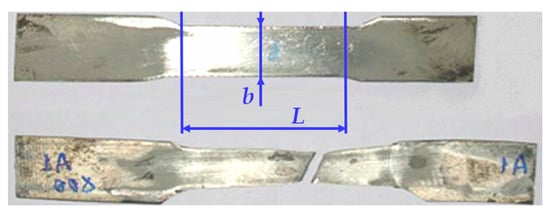
Figure 1.
Specimens used to determine the mechanical characteristics of the material.
The following samples were tested:
- Six plates produced from the original material;
- Six plates produced from the material hardened by plastic deformation;
- Six plates produced of the thermally treated (annealed) material.
The example of the M2O steel tensile diagram obtained during the experiments is presented in Figure 2.
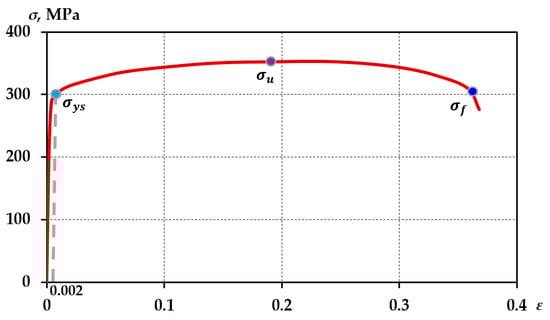
Figure 2.
Single uniaxial tensile deformation diagram of steel M2O.
During design of the numerical model of the thin-walled elements subjected to buckling in the LS-DYNA software package, the material was described by using the two most common models describing the behaviour of the material in the elastoplastic zone. Figure 3 presents tensile diagrams of material M2O (σys = 296.7 MPA, σu = 430 MPA) approximated by different laws: by approximating with tangent modulus ET = 491 MPA; approximating with exponential hardening function without accounting for the real stress at break values k = 525, n = 0.1123; and approximating with exponential hardening functions by accounting for the real stress at break value, k = 580, n = 0.184.
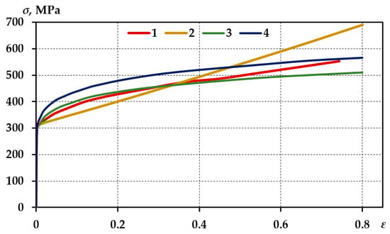
Figure 3.
Approximation of points of the tensile diagram of material M2O by various laws; (1—the actual stress and deformation curve; 2—approximated with tangent modulus; 3—approximated with exponential hardening function without accounting for the real stress at break values; 4—approximated with exponential hardening function by accounting for the real stress at break value).
The first model is based on the law of linear hardening. The linear hardening relationship (Figure 3, curve (2)) between stresses and deformations is expressed in the model as follows:
The ET module may be determined by the value of ultimate strength:
The second model is based on the exponential hardening function (Figure 3, curves (3) and (4)). In this model, the relationship between the stresses and deformations is expressed as follows:
This model provides a more accurate description of the properties of the material, but is more complicated in terms of the determination of the parameters that describe the law. The methodology of two (σy, σu, εy, εu) or three (σy, σu, σf, εy, εu, εf) characteristic points used in the LS-DYNA software package was applied to the determination of the parameters of the second model.
The approximation quality was assessed using the mean squared deviation:
The obtained results are provided in Table 1.

Table 1.
Approximation quality of different descriptions of material properties.
Exponential dependence obtained without accounting for the real burst stresses had the best correspondence to the experiment results (Figure 3, curve (3)).
During the in situ experiments it was noticed that, with the section buckling the material was noticed to not deform up to the breaking strength, and the tangent model and two-point exponential model described the initial part of plastic deformation with similar accuracy. Therefore, additional numerical experiments were conducted. Their results are provided in Figure 4. It was noticed that the results of description of material characteristics using the exponential hardening function and evaluation of the breaking stresses had the lowest correspondence to the real experiment results. Using these descriptions of the material characteristics, the results obtained were close and differed insignificantly from each other. Therefore, in subsequent calculations, the description according to the linear hardening law, which was easier to determine and sufficiently accurate, was used for the description of the material.
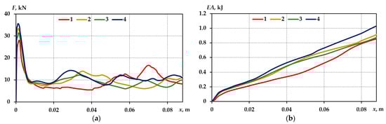
Figure 4.
Buckling force (a) and absorbed energy (b) diagrams of the T1 section element, when the material is approximated with different descriptions; (1—in situ experiment; 2—by approximation with tangent modulus; 3—by approximation with exponential hardening function without accounting for the values of true stresses at break; 4—by approximation with exponential hardening function by accounting for the value of true stresses at break).
Additional investigations were conducted to assess the process-related factors. For the design of the numerical model of the sample with a rectangular or other cross-sectional shape and with spot-welded joints and being subjected to buckling, forces required to break the spot-welded joint in axial and longitudinal (shear) direction must be available in addition to the material properties. For this purpose, the specimens (Figure 5) were produced according to the specifications of the vehicle design guide [47]. The shear and axial forces necessary to break the joint were measured for the specimens by quasi-static tensile tests using the universal 50 kN UMM-5T testing machine (Kaunas University of Technology, Kaunas, Lithuania).
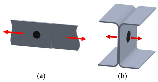
Figure 5.
Shape of the spot welded joint for determining the characteristics of the specimens: for the shear force (a); for the axial force (b).
2.2. Quasi-Static Investigation of Buckling of the Part of Crumpling Zone
The investigation aimed to identify the effect of damages of crumple zone elements damaged during a traffic accident and subjected to post-accident repair on the amount of absorbed energy of the longitudinal members under different types of load. For the investigation, a fragment of the Toyota Echo crumpling zone with initial length L = 170 mm was chosen. The specimen consisted of two parts joined by spot welding. The diameter of the spot-welded joint was 5 mm. The specimen featured eight spot-welded joints. The spot-welded joints were positioned symmetrically (Figure 6a).
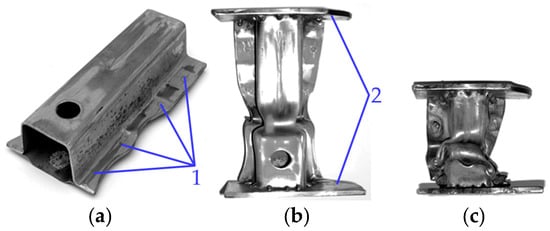
Figure 6.
P1 specimen used for the experiment: before the test (a); after the first test (b); after the second test (c); (1—positions of the spot-welded joints; 2—fixing plates).
The wall thickness of the parts was thk1 = 1.4 mm and thk2 = 0.7 mm. For accurate positioning and uniform distribution of the load of the sample during the experiment, 10 mm thick alignment plates had been welded to the ends of the specimen (Figure 6b). The experiments confirmed that the plates provided uniform and perpendicular load distribution in relation to the specimen cross-section during the experiment.
According to Figure 7, the critical buckling force Fcr,1 = 46 kN was reached during the first experiment. During repeated buckling of the sample, the critical buckling force achieved was Fcr,2 = 37 kN, that is, 20% lower than during the first experiment. Meanwhile, the amount of absorbed energy calculated after specimen deformation at a distance of 17.5 mm distance decreased by only 5% (EA1 = 390 J, EA2 = 370 J).
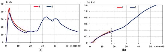
Figure 7.
Deformation forces obtained during quasi-static experiments: axial displacement diagrams (a) and absorbed energy amount-axial displacement diagrams (b); (1—original part; 2—part with the restored geometry).
The quasi-static in situ experiments performed on the crumple zone part of a Toyota Echo showed the following:
- Critical buckling force decreased by 20% during the quasi-static buckling of the specimen with the restored geometry;
- The amount of absorbed energy decreased by 5% after the specimen to the same length;
- Theoretical assumptions on the effect of minor geometric deviations on the amount of absorbed energy in case of considerable deformations were verified.
Even where the crumple zone elements are carefully and thoroughly straightened back, they could be claimed to have unevenness which may be expressed in the numerical models as 1 mm deflections directed inside.
2.3. Damage Simulation Specimens
Type T1 specimens were used for the investigation of changes taking place during the longitudinal member repair works under dynamic load. The specimens produced for this investigation consisted of two parts joined by spot welding: a U-shaped chute and a U-shaped wall that closed the contour (Figure 8).
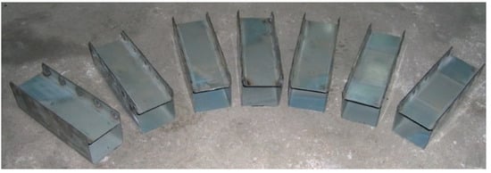
Figure 8.
T1 specimens used in the quasi-static and dynamic experiments.
The thin-walled 200 mm long element resembled the crumple zone elements used in vehicles, e.g., VW Polo, in terms of cross-section shape, structure, and assembly technique. Measurements of the specimen cross-section and layout scheme of the spot-welded joints are presented in Figure 9. A symmetrical layout of spot-welded joints was used for the specimen. The specimen had 10 spot-welded joints.
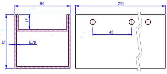
Figure 9.
Specimen T1 measurements and spot-welded joint layout sketch.
To simulate the changes in properties of the longitudinal member restored after a traffic accident, three types of specimens were used in the experiments:
- An undamaged specimen;
- A specimen cut and re-welded in the centre (Figure 10a), simulating the crumple zone part replaced during the repair;
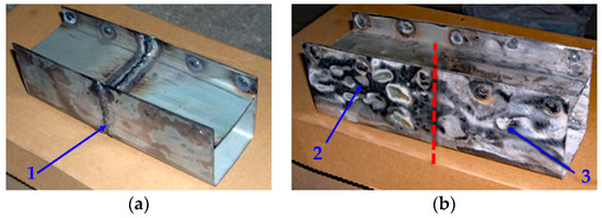 Figure 10. Specimens simulating the properties of longitudinal member restored after a traffic accident: transversely cut and welded at the centre (a); made of the material hardened by plastic deformation and annealed (b) (1—weld; 2—part of specimen made of the plastically strained material; 3—part of specimen made of annealed material).
 - specimen made of the material hardened by plastic deformation, with of the specimen span made of thermally treated material (Figure 10b). The specimen simulated the effect of minor geometric deviations and changes in the material during the repair.
To verify the applicability of the identified dependencies on elements of different cross-section shape and structures, numerical models of T2, T3, and T4 section elements were designed. They corresponded to T1 specimens by cross-sectional area, wall thickness and layout of the spot-welded joints.
2.4. Dynamic Test Methodology for Crumple Zone Elements
During the literature review, element deformations were noticed to depend on the deformation velocity and load character. To identify the dependences between quasi-static and dynamic tests, in situ experiments were performed. Dedicated test bench was made for the dynamic buckling tests (Figure A1).
The values of stress and time of the accelerometer sensors were generated and registered during the experiment. The stress values registered by the sensors during the experiment and saved on the computer were adjusted for the characteristics of the sensors used and recalculated into acceleration. The obtained acceleration—time dependences were later recalculated into force—displacement dependences. The amount of absorbed energy (area limited by the force and displacement curve) was obtained by integrating the force—displacement curve. The amount of absorbed energy was compared to the real amount of kinetic energy of the impactor mass.
After the experiments, certain specimens were noticed to be subjected to significantly greater deformations than other specimens despite the same amount of energy being absorbed. Following the visual inspection of the specimens, certain spot welds were found to have been broken in the specimens which had greater deformations. The specimens with smaller axial shortening did not have any or had significantly fewer broken welds (Figure 11).
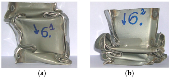
Figure 11.
Specimens after the dynamic buckling experiments: specimen without broken spot-welded joints (a); specimen with two broken spot-welded joints (b).
Axial shortening of the specimen in Figure 11a was 95 mm upon absorption of 1765 J of energy. Axial shortening of the specimen in Figure 11b was 110 mm despite the same amount of energy being absorbed (1765 J).
The conducted quasi-static and dynamic buckling experiments on the specimens showed the following:
- During buckling of the specimens using the dynamic load, the amount of energy absorbed was % greater than under quasi-static buckling;
- Irrespective of the type of specimens simulating the repair of crumple zones of various kinds, the same amount of energy was absorbed per length unit in the case of quasi-static buckling;
- In the case of dynamic loading, the specimens of different types were subjected to the same degree of deformation under the dynamic load of the same character (initial velocity and mass).
3. Methods
3.1. Dynamic Models of Distributed Masses of Crumple Zone Elements
Software developed at the Department of Transport Engineering at Kaunas University of Technology was used for verification of functionality of characteristics of the crumple zone elements and the effect of change in their properties.
Dynamic models of distributed masses are the basic models for the assessment of impact loads. They were used in this study to assess the contribution of an individual crumple zone to the overall energy absorption process during impact.
Although the three-mass dynamic model is one of the simplest, it provides a fairly accurate reflection of the key properties of the front crumple zone of a vehicle. The distribution of the model into three zones is conditional. Each part reflects a certain group of elements that includes the assemblies located in the respective zone. The generalized mass of the elements located within the zone is attributed to the respective zone. The methodology for determining the generalized mass is not strictly defined. Usually, it is considered to be the mass of key elements of the zone and the vehicle units/assemblies connected thereto. During the development of the research methodology, the guidelines provided in [48] were applied to the control of mass distribution. That is, the sum of the masses of the first and second zones was about 33% of the vehicle mass, and the mass of the third zone was about 66% of the vehicle mass. The characteristics of the zone, i.e., the rigidity and damping coefficients, were determined in view of the character of connection between the elements (series, parallel, or mixed). The three-mass dynamic model allowed the authors to identify the key weaknesses in the modelling. One of the most important weaknesses was the impossibility of describing zone deformation properties using linear elasticity elements at higher velocities. These elements would only be applicable before the emergence of plastic deformations, for example, when calculating the bumper zone of a US-type vehicle. For this purpose, the methodology for the determination of the element characteristics and the application specifications and efficiency of the four-mass models (Figure 12) had to be adjusted.
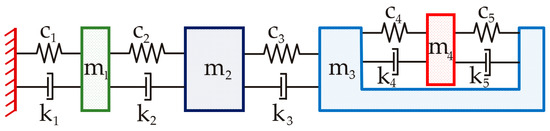
Figure 12.
Four-mass dynamic model.
A fourth mass—vehicle crew (m4)—is used in the four-mass dynamic model. The relationships in the model reflect the effect of vehicle safety systems (seats, safety belts, air bags, etc.). The relationships between the 3rd and 4th parts are reflected by parameters C4, k4, C5, k5: C4 and k4 depend on the properties of the safety belts, while C5 and k4 are determined by the properties of the seat backrest. The behaviour of the four-mass dynamic model is described by a system of differential equations:
The parameters used in these models were Ci, ki, Fcri and xlim. Zone damping coefficient ki was accepted as constant and independent from the value of deformations. There is no rationale behind description of the crumple zone properties using elastic elements only, as this would distort the rebound process that has considerable effect on the entire process. Hence, plastic elements were introduced into the models describing the crumple zones. The characteristics of plastic elements are described by Fcri. Stiffness coefficients Ci are determined by element deformation to Fcri. The stiffness value was adjusted where deceleration was greater than 100 g at the initial impact moment. During investigation of a real structure, Fcri is calculated according to the condition of loss of stability of the crumple zone element. Rebound characteristics were introduced additionally as they enabled modelling of the zone deformations under decreasing load (Figure 13).
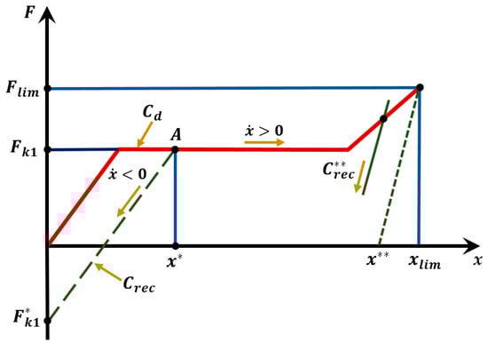
Figure 13.
Description of element deformations used in the dynamic model of distributed masses.
The adjustment of description of the crumple zone properties enabled more accurate reflection of the effect of changes in element properties on the deformation process of the entire crumple zone and on the overloading of the part of the 3rd crumple zone that was directly related to the crew. In this case, the elastic deformation model was used before plastic deformation emerged. After the plastic deformation started, the deformation progress calculation was altered depending on the process velocity: if then ; if then . During the change of the deformation velocity sign, value was registered, and the calculation was then performed using , irrespective of the sign, until the value was higher than x*. After x* had been reached, the deformation process returned to the former conditions and .
When modelling the front collision, it was noticed that there could be cases where, with the vehicle moving back from the obstacle (usually at the end of the impact process), the force acting on the first element of the zone would be negative. Hence, additional condition was introduced into the model, and for this case, the deformation force, element rigidity, and damping were assumed to be equal to zero.
In preparation for a more accurate description of deformation of the crumple zone elements, the final zone deformation by its complete squashing was taken into consideration. In this case, the zone became more rigid, and increase in rigidity of the zone was modelled under the assumption that Fcri was achieved by imposing elastic deformation on the remaining part of the crumple zone. The new rigidity C value at the plastic deformation value x** was determined as follows:
Limitation was set for C** value in order to determine recoverable elastic deformations and not exceed xlim. Additional equation correction was introduced into the calculation of the forces acting on the third element of the crumple zone. In this case, it was assumed that, with the start of deformation of the third element during the collision, front wheels would be blocked due to the vehicle body damages, and the third zone would be under the action of the friction force, the maximum value of which was:
The modulus of force was compared to force Fc23, acting between the 2nd and 3rd zones due to element elasticity. It was assumed that if Fc23 > Ffr max then Ffr > Ffr max; if Fc23 < Ffr max then Ffr = Ffr max.
The amount of the absorbed energy was obtained having estimated the area, restricted with a force—shift diagram:
The adjustment of the description of the crumple zone properties enabled more accurate reflection of the effect of changes in element properties on the deformation process of the entire crumple zone and on the overloading of the part of the 3rd crumple zone that was directly related to the crew.
3.2. Finite Element (FE) Models of Crumple Zones
In this paper, FE models were developed for the simulation of quasi-static experiments according to the geometric measurements of the specimen used in the in situ experiments with the FE software LS-Dyna V.971. Nodes located on the bottom of the specimen were fixed in all directions x, y, and z. For nodes located at another end of the specimen, the command ‘BOUNDARY_PRESCRIBED _MOTION_SET’ [49] was used to set the constant motion speed (v = 5 m/s) in the vertical direction y, and maximum possible displacement was set for the nodes. During deformation, the command ‘CONTACT_AUTOMATIC_SINGLE_SURFACE’ [49] was used for simulation of the contacting surfaces of the element. Potential displacement during straightening out of the longitudinal member was introduced as the deflection directed inside. These geometric deviations were simulated in the model by sliding the respective nodes in x and/or z directions.
For modelling the dynamic loading experiments, the nodes located on the bottom of the specimen were connected to the fixed plate referred to as S4 in the model. Moreover, plate S3 was designed to impact the investigated specimen. The load was created by attributing the required mass and initial velocity ‘INITIAL_VELOCITY‘ to plate S3 nodes. Spot-welded joints ‘CONSTRAINED_SPOTWELD_ID‘ were designed in the model. For each joint, parameters SN (force in axial direction) and SS (force in shear direction) were entered. In the model, one spot-welded joint had eight nodes, i.e., four pairs of two interconnected nodes. In this case, the value entered for SN and SS in the LS-Dyna subprogram was equal to ¼ of the value of the forces obtained during the in situ experiments.
During modelling of buckling of the thin-walled structural element, Belytschko–Tsay finite shell elements were used and calculated according to the thick-walled Mindlin–Reissner plate theory. With the deformation velocity increasing, a zero deformation energy (hourglass) effect may emerge in the model, and additional control was set for the elements to avoid this effect. To assess the effect of finite element mesh density, numerical models corresponding to the specimen simulated in Section 2 were designed for elements of different sizes. As a result of the numerical experiments, the finite element mesh density was found to not have any substantial effect on the form of specimen deformation. Figure 14 presents 30 mm, 60 mm and shapes of the specimen deformed at the maximum length. Based on the studies conducted, a 4 mm finite element was selected for development of subsequent models. The selection was based on the following criteria:
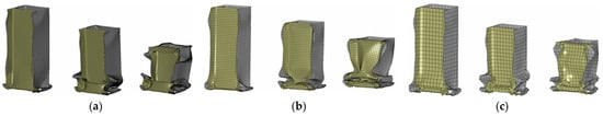
Figure 14.
30 mm, 60 mm and specimen with maximum deformations: (a)—2 mm square finite element; (b)—4 mm finite element; (c)—8 mm finite element.
- The results obtained with the models were very close to the results of the in situ experiments;
- Enabled determination of fabricated joints as accurately as possible;
- Acceptable duration of computer calculation.
4. Results
4.1. Analysis of Results Obtained with the Dynamic Models of Distributed Masses
The elements of the front crumple zone of a Toyota Yaris (year 2007) were chosen as the modelling object (Figure 15). There are many non-genuine spare parts attributable to crumple zone elements produced for this vehicle. This study aimed at verifying the rationale of the use of these elements.
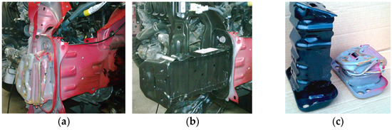
Figure 15.
Toyota Yaris crumple zones: deformed after crash (a), recovered after crash (b), crumple zone elements for energy absorption (c).
During the repair of this vehicle, the mentioned non-genuine crumple zone elements were used, while the longitudinal member was straightened back. Consequently, this kind of repair results in completely different crumple zone parameters. Hence, after the repair works, the car may have substantial hidden, or even life-threatening, changes. Calculations using the SMUG94 software developed at the Department of Transport Engineering at Kaunas University of Technology were carried out at two different velocities: 30 km/h and 64 km/h. We chose 64 km/h as it is the limit velocity at which the driver and crew would still survive in the event of a front collision with a fixed obstacle. The crumple zone parameters were determined by measuring the cross-sections of crumple zone elements. Limit loads were determined according to the loss of stability by the crumple zone. The initial calculation data are presented in Table 2.
Table 2.
Calculation data for Toyota Yaris.
After definition of the methodology of grouping the elements into crumple zones and determination of the crumple zone parameters mi, Ci, ki, Fcri, xlim, it became possible to model the process of deformation of the entire crumple zone during impact. Three calculation variants were performed: variant 1—standard parameters of all three zones; variant 2—standard parameters of the 2nd and 3rd zones, 1st zone consisting of non-genuine parts; variant 3—standard parameters of the 3rd zone, 1st zone consisting of non-genuine parts, 2nd zone rigidity lower than 30%. Variant 3 was selected because, in cases where the 1st zone needs replacement, the 2nd zone is usually also subjected to deformations.
The results obtained when modelling a traffic accident with a Toyota Yaris at initial velocity with obstacle equal to 64 km/h are presented in Figure 16.
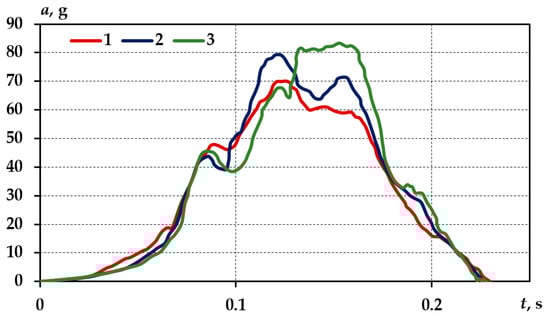
Figure 16.
Overloads acting in the 3rd crumple zone at initial collision velocity 64 km/m; (1—original parameters of all the zones; 2—1st zone consisting of non-genuine parts; 3—1st zone consisting of non-genuine parts, 2nd zone stiffness lower than 30%).
In this case, the overload values were already hazardous to the car crew. The determined head injury criteria (HIC) [50,51] values in all three cases of crumple zone configuration were: in case of standard crumple zone elements—HIC = 640, non- genuine 1st zone parts—HIC = 607, and the third variant—HIC = 700.
4.2. Investigation of the Effect of Quasi-Static Buckling and Geometric Deviation of the Damaged Crumple Zone on the Specimen Deformation
The analysis of results generated by the dynamic models has shown that the descriptions of characteristics of crumple zone elements need to be adjusted. The geometry and structure of the modelled element corresponded to the specimen P1 of the crumple zone fragment of a Toyota Yaris used during the quasi-static in situ buckling experiments. The cross-section area of the specimen was equal to 256 mm2.
The following types of numerical models for specimens P1 were designed:
- The original element model;
- A model simulating the specimen with the material strengthened in the plastic deformation wave span used during the repeated experiment, and 0.5 mm geometric deviation from the initial shape was introduced;
- A specimen model of original characteristics with 0.5 mm geometric deviation;
- A specimen model of original characteristics with 1 mm geometric deviation;
- A specimen model of original characteristics with 0.5 mm geometric deviation in the bottom part of the specimen;
- A specimen model of original characteristics with 1 mm geometric deviation in the bottom part of the specimen.
The mechanical characteristics of the materials determined under the methodology of Section 2 are presented in Table A1, and the mechanical characteristics of fabricated joints are presented in Table A2. Figure 17 suggests that the geometric deviation of 0.5 mm did not have any effect on the nature of specimen deformation (Figure 17c,e) and the first plastic deformation wave emerged at the same location as in the original geometry (Figure 17a).
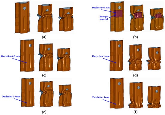
Figure 17.
Initial shapes, 20 mm and 40 mm deformed specimen deformation shapes: model of the specimen of original characteristics (a); model simulating the specimen used during the repeated buckling experiment—material M1D in the first deformation wave range and with a geometric deviation of 0.5 mm introduced (b); model of the specimen of original characteristics with 0.5 mm geometric deviation (c); model of the specimen of original characteristics with 1 mm geometric deviation (d); model of the specimen of original characteristics with 0.5 mm geometric deviation in the bottom part of the specimen (e); model of the specimen of original characteristics with 1 mm geometric deviation in the bottom part of the specimen (f).
The resulting deformation forces—axial specimen shortening diagrams—are similar in nature (Figure 18, curves (1) and (3)), and the formed first and second plastic deformation wave lengths remained unchanged.
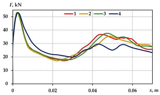
Figure 18.
Force—deformation diagrams (FEM) of different types of specimens of section P1; (1—original geometry and original material; 2—0.5 mm geometric deviation and material subjected to plastic deformation; 3—0.5 mm geometric deviation and original material; 4—1 mm geometric deviation and original material).
The amounts of absorbed energy were also virtually identical. Meanwhile, the geometric deviation of 1 mm altered the location of formation of the first plastic deformation wave in the specimen (Figure 17d,f). The geometric deviation of 1 mm influenced the location of formation of the first plastic deformation wave, thus altering the nature of the deformation force–axial specimen shortening diagram and the formed wave lengths (Figure 18, curves (1) and (4)). Whereas the cross-section shape of the specimen was similar across the length of the specimen, the amount of energy absorbed by the specimen changed very insignificantly irrespective of the location of formation of the first plastic deformation waves. In this case, at axial shortening of the specimen 80 mm, the specimen of original geometry absorbed 1.88 kJ energy, while the specimen with 1 mm geometric deviation which caused the location of formation of the first plastic deformation waves and the wave lengths absorbed 1.75 kJ energy at the same axial shortening of the specimen.
4.3. Investigation of the Effect of the Crumple Zone Element Properties Changed during the Repair on the Buckling Characteristics under the Dynamic Load
Following verification of the effectiveness of FEM in forecasting of the quasi-static test results, the possibilities of the effect of dynamic loads and the modelling thereof were investigated. Three types of specimen of the T1 section described in Section 2 were used during the numerical experiments.
The preliminary value of the average buckling force of specimen T1 was calculated analytically using two popular expressions proposed by Abramowicz and Jones [52,53]:
Ohkubo [54] proposed the following expression for calculation of the mean force of thin-walled square columns joined by spot welding:
The mean buckling force was calculated using the expressions Equations (11) and (12): Faver = 11.8 kN. According to Equation (13), the average buckling force: Faver = 21.05 kN. The mean buckling force and amount of absorbed energy per material volume unit (with specimen deformation equal to 85.37 mm) obtained during the quasi-static experiments were: Faver,st1 = 9.78 kN; EAv1 = 43.84 kJ/m3; Faver,st2 = 9.66 kN; EAv2 = 43.31 kJ/m3; Faver,st3 = 9.77 kN; EAv3 = 43.84 kJ/m3.
The following was noticed after comparing the average buckling forces generated by the expressions during the in situ experiments of quasi-static buckling to the average buckling forces generated by the expressions proposed by different authors:
- The average buckling force value obtained according to Equations (11) and (12) proposed by Abramowicz and Jones was close to the value obtained during the in situ experiments, i.e., was only 20% higher;
- The average buckling force value obtained according to Equation (13) proposed by Ohkubo was more than twice that obtained during the in situ experiments.
Based on the experimental data obtained, the effect of welded joints and straightening process, as possible changes of properties, on the buckling force value was insignificant. The dynamic loading tests were conducted under the methodology of dynamic buckling experiments described in Section 2 and by using the same three types of specimens as in the quasi-static experiments. The dynamic coefficient is often used in analytical calculations because it accounts for the effect of dynamic loading on the structure. The dynamic coefficient depends on the nature of the load, the geometric and structural characteristics of the element subjected to buckling, and on the material. The dynamic coefficient is usually obtained by dividing the average buckling force under dynamic load by the average buckling force under static load:
The average buckling forces of the specimens obtained during the numerical experiments of quasi-static and dynamic buckling are compared in Figure 19. In this case, the average buckling value obtained during quasi-static buckling of an undamaged specimen was accepted as 100%.
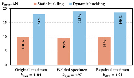
Figure 19.
Dependence of the average buckling force on the nature of the load.
Of the results presented in Figure 19 it was noticed that, when subjected to dynamic buckling and axial shortening by 0.0854 m of the specimen, each specimen absorbed approximately 90% more energy compared to quasi-static buckling: the undamaged specimen absorbed 84% more energy, the welded specimen 97%, and the damaged specimen 91%. It was also noticed that there was only a slight difference in the amount of energy absorbed by all three specimens under the same buckling conditions. The main parameters obtained during the numerical experiments of quasi-static and dynamic buckling are presented in Table 3.
Table 3.
The main parameters of specimen buckling obtained during numerical experiments and calculated under axial shortening 0.0854 m of the specimen.
The calculated dynamic coefficient could be applied to the modelling of the front crumple zones of cars by using dynamic models of distributed masses described in Section 3. With the dynamic coefficient value available, it would be sufficient to conduct quasi-static in situ experiments by determining the rigidity characteristics of a certain part of the crumple zone, and then multiply the element rigidity characteristics by this coefficient. However, it is important to note that the identified dynamic coefficients would accurately apply only in cases where they were applied to identical elements (identical by geometry, structure, and material properties) and only under the same nature of load and deformation (deformation velocity, axial shortening of the specimen).
4.4. Investigation of the Effect of Characteristics of Spot-Welded Joints on the Crumple Zone Buckling
The results provided by the numerical experiments showed that, in order to assess the effect of damages occurring during the repair, it is necessary to design the methodology to assess the effect of the characteristics of welded joints on the process of the elements of the deformation of crumple zone using the numerical methods.
The in situ experiments were conducted to determine the mechanical characteristics of material M1O of the specimen used during the quasi-static and dynamic in situ experiments M1O (Table A1) and original spot weld Spw1O and manual spot weld Spw1M joints (0.78 mm thick metal sheets joined by spot welding) (Table A2). The FEM numerical model was designed according to the geometric measurements of the specimen used in the in situ experiments of quasi-static and dynamic buckling and the methodology in Section 2. In the first case of modelling, as during the in situ experiments, an initial velocity of 7.67 m/s and a mass of 60 kg were set for the loading plate. Then, the effect of the weakened spot-welded joints on the deformation of the specimen was modelled under the dynamic loading of the same nature. The positions and numbering of the spot-welded joints in the model are presented in Figure 20.
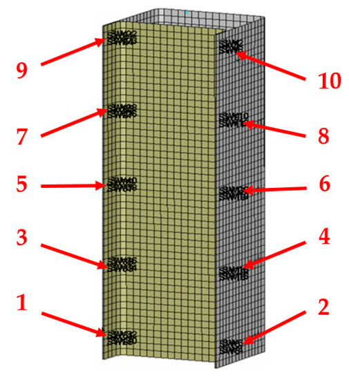
Figure 20.
Positions and labelling (Table A3) of the spot-welded joints in the FE model.
The model was calculated by amending certain weld parameters. The key buckling parameters under various layout variants of spot-welded joints of different characteristics are presented in Table A3. In the analysis of the results, the changed characteristics of the spot-welded joints located in the zone of formation of plastic deformation waves have a considerable effect on the nature of the deformation of specimen and the amount of the energy absorbed per unit of length (Figure 21).
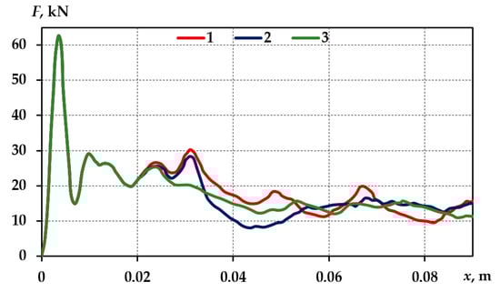
The deformation force—axial shortening is reported for the specimen of original characteristics, the specimen with the 3rd and 4th spot weld positions 50% axially weakened, and the specimen with the 5th and 6th spot welds not welded. Figure 21 suggests that the weakened spot-welded joints or absence thereof led to the altered nature of the buckling diagram during formation of the second buckling wave. This suggests that the wave length and amount of absorbed energy per length unit were changing (mean buckling force). Figure 22 shows the dependencies of the absorbed energy amount on the axial shortening for the three types of specimens.
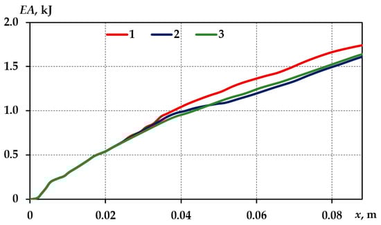
Figure 22.
Absorbed energy–axial displacement diagrams of different types of section T1 specimens; (1—original characteristics of all spot-welded joints; 2—manual welding in the 2nd, 3rd and 4th positions; 3—no joints in 3rd–5th and 6th positions).
Figure 22 suggests that in the case of weakened spot-welded joints in the 3rd and 4th positions, the axial shortening of the sample where the amount of energy absorbed was increased to 0.104 m. Meanwhile, the axial shortening of the specimen with all the spot-welded joints having original characteristics with the same amount of energy absorbed (1765 J) was 0.0962 m. The specimen with manual welded joints in the 3rd and 4th positions, following deformation of 0.0962 m, absorbed 1620 J, i.e., 8% less energy. The dependences of the mean buckling force of these types of specimens on the initial load velocity and at constant deformation velocity, generated by the FEM model, are presented in Figure 23.
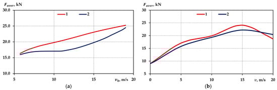
Figure 23.
Dependence of the mean buckling force on the nature of the deformation load: dependences on the initial load velocity during the impact 60 kg (a); dependences on the constant deformation velocity (b); (1—specimen with all spot-welded joints having original characteristics; 2—specimen with manual welded joints in the 3rd and 4th positions (Figure 20).
Doubling of the initial impact velocity of dynamic loading to 15.34 m/s while maintaining the same amount of energy led to reduction in the axial shortening of the specimen of original characteristics down to 0.076 m, i.e., the absorbed energy amount per length unit increased by 25%. An increase in the initial impact velocity led to an even more evident effect of the weakened spot-welded joints on the amount of energy absorbed by the sample. Under the same dynamic load, the specimen with weakened spot-welded joints in the 3rd and 4th positions 50%, with the same amount of energy absorbed, was deformed at the distance of 0.088 m, i.e., 16% more than in the case of the specimen of original characteristics.
4.5. The Effect of Damaged Crumple Zone Part on the Vehicle Dynamic Processes
In this section, an investigation of the effect of damaged crumple zone on vehicle safety was conducted. For this investigation, an application developed on the basis of a four-mass dynamic model was used. In the application, a smaller distribution of force-deformation dependences was used for the description of the crumple zone rigidity characteristics. The stiffness characteristics of the part of crumple zone were described by its buckling force-displacement diagram approximated by an eight-point linear dependence. This method for describing the rigidity characteristics of the crumple zone enabled a more appropriate use of the buckling force dependences obtained during the in situ experiments or by using the numerical models.
The modelling was performed using the chosen characteristics of the buckling forces. The model simulated the collision of the investigated vehicle with a fixed barrier at full frontal width, which corresponded to the National Highway Traffic Safety Administration (NHTSA) methodology. This kind of collision was chosen as, in this case, the longitudinal side-members were subject to the largest share of the absorbed energy, and the longitudinal member loading conditions caused their axially symmetric deformation. The buckling force–displacement diagrams used in the model were obtained under exactly the same load nature. Accelerations of the 3rd zone with the 2nd part having original characteristics and characteristics with post-repair damage are presented in Figure 24.
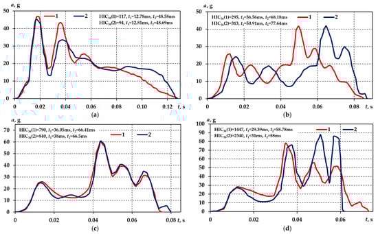
Figure 24.
Accelerations of the 3rd zone at different collision velocities: 40 km/h (a), 50 km/h (b), 64 km/h (c), 75 km/h (d); (1—2nd zone of original characteristics; 2—damaged 2nd zone).
Following the calculation of the HIC36 parameter [50,51] based on the acceleration diagrams in Figure 24, at 40 km/h collision velocity and 2nd zone of original characteristics: HIC 117; at the damaged 2nd zone: HIC 94, at 50 km/h—295 and 313, at 64 km/h—790 and 840, at 75 km/h—1447 and 2340.
Figure 25 shows time-dependent distribution of the amount of energy absorbed by individual crumple zone parts with different characteristics of the 2nd zone.
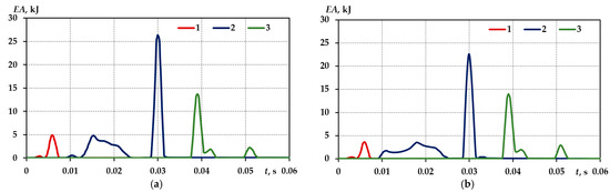
Figure 25.
Time-dependent distribution of the energy amount absorbed by the zones: with the 2nd zone of original characteristics (a); with the damaged 2nd zone (b); (1—1st zone; 2—2nd zone; 3—3rd zone).
Changes in the characteristics of the crumple zone elements were clearly recorded with the change of the initial impact velocity. The results obtained by using the distributed mass elements were partially repeated. At lower velocities, the weaker 1st and 2nd crumple zone parts absorbed the energy more uniformly. As velocity increased, the effect was reduced. As soon as the 64 km/h velocity was exceeded, the energy was absorbed by the more rigid 3rd zone, and the overloads acting on the crew increased.
The investigations found the following:
- The obtained acceleration–time dependences were closer to the in situ experiment results where adjusted crumple zone element characteristics were used; (Figure 25);
- The adjusted model enabled more accurate forecasting of the effect of individual elements on the course of deformation of the crumple zone;
- The weakening of the parts of the 1st and 2nd crumple zones had a negative effect on the car safety of the vehicle at collision speeds of 50 km/h and higher. With increasing collision velocity, the negative effect became more evident.
5. Conclusions
Based on these results, the following observations have been made.
A dynamic model that assesses the effect of individual regions of crumple zones on the overall deformation process was run. The course of deformation of the regions and the amount of energy absorbed were found to be affected by the adjacent regions. Therefore, damages in one zone may influence the overall deformation process. To assess the effectiveness of the crumple zone, it is necessary to analyse the collision velocities of different ranges: up to 50 km/h and above 50 km/h.
The quasi-static and dynamic in situ experiments of part of crumple zone have demonstrated that damages alter the element’s characteristics. During the quasi-static buckling of the specimen of restored geometry, the critical buckling force was reduced by 20% and the amount of absorbed energy was reduced by 5% with the specimen deformed to the same length. The experiments conducted on specimen buckling have demonstrated that, with the specimen subjected to buckling under dynamic load, the amount of energy absorbed by them is 90% higher than under quasi-static buckling.
The effect of geometric deviations on the course of element deformation was found to be inconclusive. The effect of a single 0.5 mm geometric deviation was insignificant. Meanwhile, a 1.0 mm single deviation altered the location of formation of the first plastic deformation wave, but did not have any significant effect on the absorbed energy amount per length unit.
The results obtained by numerical models corresponded to the results of the in situ experiments. To describe the damage of crumple zone elements, it is sufficient to adjust the descriptions of the materials and fabricated joints.
During the modelling, the altered characteristics of the spot-welded joints, irrespective of their positions, were found to have the capacity to considerably influence the nature of the specimen deformation and amount of energy absorbed. The amount of energy absorbed decreased by 8% after the spot-welded joints were weakened by 50% in the middle zone of the specimen used during the experiment and deformation of the specimen to 1/2 length. With the element absorbing 1.77 kJ of energy, the axial shortening of the specimen subjected to buckling increased by 9% compared to the specimen with all original spot-welded joints. The axial weakening of the spot-welded joints located in the zone of formation of the first plastic deformation waves by 50% was equivalent to the absence thereof.
Non-standard parts of the crumple zone used during the repair had a considerable effect on the vehicle safety. The HIC parameter almost doubled where non-standard parts were used and the crumple zone was repaired.
The effect of changes in the characteristics of individual crumple zone regions on their functionality was determined:
- An increase in stiffness of the 1st and 2nd crumple zone elements had a negative effect on car safety throughout the interval of investigated velocities. When the collision velocity increased, the negative effect decreased, but still remained considerable.
- The reduction in stiffness of the 1st and 2nd crumple zone elements had a positive effect on the car safety at collision velocities up to 67 km/h. At higher velocities, weakening of the crumple zone elements had a negative effect on the car safety, and the effect continued increasing with the increasing collision velocity.
Author Contributions
Conceptualization, D.J. and V.L.; methodology, D.J. and V.L.; software, V.L.; validation, D.J., V.L. and A.K.; formal analysis, D.J., V.L. and A.K.; investigation, D.J., V.L, A.K. and R.M.; resources, R.M.; data curation, D.J., V.L, A.K. and R.M.; writing—original draft preparation, D.J., V.L. and A.K.; writing—review and editing, D.J., V.L. and A.K.; visualization, V.L.; supervision, D.J., V.L., A.K. and R.M.; project administration, R.M. All authors have read and agreed to the published version of the manuscript.
Funding
This research received no external funding.
Institutional Review Board Statement
Not applicable.
Informed Consent Statement
Not applicable.
Data Availability Statement
Not applicable.
Conflicts of Interest
The authors declare no conflict of interest.
Nomenclature
| Latin symbols | |
| acceleration (g); | |
| specimen test part width (mm); | |
| crumple zone stiffness (kN/m); | |
| crumple zone stiffness variation (kN/m); | |
| element stiffness during progression of deformation (may be negative) (kN/m); | |
| stiffness during rebound (elastic deformation) is set at the beginning of calculation for each part of the force-deformation dependence (kN/m); | |
| coefficient of variation; | |
| dispersion; | |
| elastic modulus (MPa); | |
| absorbed energy (kJ); | |
| the amount of energy absorbed per unit volume of material (kJ/m3); | |
| tangent modulus (MPa); | |
| force (kN); | |
| average buckling force (kN); | |
| average buckling force under dynamic load (kN); | |
| average buckling force under dynamic load (kN); | |
| critical buckling force (kN); | |
| the force acting between 2nd and 3rd crumple zones (kN); | |
| critical force that causes plastic deformation of the crumple zone element upon its application (kN); | |
| critical force correction due to the altered elastic characteristics (kN); | |
| crumple zone critical force values (kN); | |
| the force corresponding to a point A (kN); | |
| limit value of the critical force (kN); | |
| friction force and maximum value of friction force, respectively (kN); | |
| specimen test part height (mm) [52]; | |
| hardening coefficient; | |
| dynamic coefficient; | |
| crumple zone damping coefficients (kN*s/m); | |
| bending energy correction factor [52]. The calculation assumes ; | |
| decreasing wavelength [52]. The calculation assumes ; | |
| specimen test part length (mm); | |
| crumple zone masses (kg); | |
| plastic moment (N*m); | |
| M1O, M2O | original material specimens; |
| M1D | plastically strained specimens; |
| M1A | annealed specimens; |
| work hardening exponent or strain hardening exponent; | |
| the total number of samples; | |
| P1 | specimens for buckling simulation; |
| radius of rounding of profile corners [52]. The calculation assumes r ; | |
| standard deviation; | |
| Spw1O | original spot weld; |
| Spw1M | manual spot weld; |
| distance between spot welding joints (mm) [52]; | |
| time (s); | |
| wall thickness of the specimen (mm); | |
| T1,T2,T3,T4 | specimens for damage simulation; |
| displacement (m); | |
| width of the joining flange (mm) [52]; | |
| sample mean; | |
| plastic deformation at the calculation time moment (%); | |
| the derivative of the crumple zone displacement, velocity (m/s); | |
| crumple zone stiffness variation (kN/m); | |
| limit value of plastic deformation of the crumple zone element; when the limit value is reached, only elastic deformations of the crumple zone are possible; | |
| residual displacement at point A; | |
| Greek symbols | |
| coefficient accounting for the increase in rigidity of the crumple zone; | |
| strain (%); | |
| strain at fracture(%); | |
| tensile yield strain (%); | |
| 0.2% plastic strain (%); | |
| ultimate true strain (%); | |
| friction coefficient; | |
| stress (MPa); | |
| experimental stress value (MPa); | |
| fracture strength (MPa); | |
| elastic limit or yield strength, the stress at which 0.2% plastic strain occurs (MPa); | |
| tensile yield stress (MPa); | |
| ultimate tensile stress (MPa); | |
| theoretical stress value (MPa); | |
| ultimate true stress (MPa); | |
Appendix A
The impact test bench (Figure A1) consisted of the base (1), a 12 mm diameter guiding rod (2), an impactor of 60 kg (3). Under the action, the force of its own weight develops, the impactor mass develops a certain speed, and impacts the specimen. The highest acting force of aerodynamic drag at velocity v = 7.67 m/s, equal to 2.88 N. This accounts for only 0.5% of the impactor body weight force, and the effect of air drag force on the velocity of impactor body velocity was not evaluated. The specimen was impacted by a falling metal block that had the mass of 60 kg.

Figure A1.
General view of the test bench for dynamic buckling experiments; (1—test bench base; 2—guiding rod; 3—impactor body; 4—Wilcoxon 784A accelerometer sensors; 5—upper attachment point of the guiding rod; 6—alignment plate; 7—specimen; 8—rubber gasket; 9—PicoScope signal converter—3424; 10—sensors power supply device; 11—power supply device).
The acceleration–time dependences of the impactor body were registered during the experiments. The guiding rod is designed to prevent the impactor mass from deviating from its course and to ensure that it accurately hits the geometric centre of the specimen. The guide rod was screwed to the base (1) at the bottom and to the upper attachment point (5) at the top. Following the experiment and as specimen (8) was being replaced, the plant was disassembled. For accurate setup of the specimen, two alignment plates (6) were manufactured and placed at the top and bottom of the specimen. Rubber gaskets 1 mm thick were used on the top and bottom of the specimen with the alignment plates to avoid the effect of acoustic waves. This solution was chosen because, during the first tests, it was noticed that the vibrations caused by the noise waves caused fairly strong distortions of the indications registered by the sensors. The required velocity of impactor mass was set by adjusting the height from which it would be dropped accordingly. WILCOXON—784A accelerometer sensors (Wilcoxon Sensing Technologies, Frederick, MD, USA) (4) were mounted on the impactor mass. The sensor characteristics are specified in [55]. The data were registered real-time on a PC, recorded, and processed using PICOSCOPE 5.13.7 (Pico Technology, St Neots, UK) software [56].
Appendix B
Table A1.
Mechanical characteristics of materials, M1O, M1D, and M1A.
Table A1.
Mechanical characteristics of materials, M1O, M1D, and M1A.
| No | Original M1O | Plastically Strained M1D | Annealed M1A | |||||||||
|---|---|---|---|---|---|---|---|---|---|---|---|---|
| 1 | 312 | 500 | 0.182 | 610 | 352 | 510 | 0.159 | 450 | 298 | 485 | 0.192 | 590 |
| 2 | 304 | 490 | 0.169 | 660 | 351 | 500 | 0.157 | 400 | 296 | 490 | 0.191 | 640 |
| 3 | 316 | 495 | 0.172 | 590 | 354 | 510 | 0.154 | 450 | 296 | 480 | 0.186 | 600 |
| 4 | 304 | 510 | 0.176 | 750 | 348 | 490 | 0.145 | 380 | 292 | 485 | 0.187 | 650 |
| 5 | 310 | 496 | 0.176 | 620 | 344 | 495 | 0.148 | 440 | 284 | 490 | 0.179 | 760 |
| 6 | 314 | 505 | 0.169 | 680 | 348 | 500 | 0.159 | 410 | 288 | 478 | 0.181 | 660 |
| 310 | 499 | 0.174 | 650 | 349 | 501 | 0.154 | 420 | 292 | 485 | 0.186 | 650 | |
| 4.62 | 6.63 | 0.00 | 53.39 | 3.29 | 7.31 | 0.01 | 26.77 | 4.97 | 4.55 | 0.00 | 55.38 | |
| 5.06 | 7.27 | 0.01 | 58.48 | 3.61 | 8.01 | 0.01 | 29.33 | 5.44 | 4.98 | 0.01 | 60.66 | |
| 1.63 | 1.46 | 2.88 | 8.99 | 1.03 | 1.59 | 3.85 | 6.98 | 1.86 | 1.02 | 2.80 | 9.33 | |
Table A2.
Characteristics of the Spw1O and Spw1M spot-welded joints.
Table A2.
Characteristics of the Spw1O and Spw1M spot-welded joints.
| No | Original Spot Weld Spw1O * | Manual Spot Weld Spw1M ** | ||
|---|---|---|---|---|
| 1 | 9.8 | 5.6 | 9.6 | 2.1 |
| 2 | 10.2 | 6.2 | 9.4 | 1.2 |
| 3 | 9.6 | 6.5 | 9.5 | 1.8 |
| 4 | 9.8 | 4.8 | 9.6 | 0.8 |
| 5 | 10 | 5.4 | 8.6 | 2.2 |
| 6 | 9.6 | 3.9 | 9.1 | 1.6 |
| 9.8 | 5.4 | 9.3 | 1.62 | |
| 0.22 | 0.87 | 0.36 | 0.49 | |
| 0.24 | 0.95 | 0.39 | 0.54 | |
| 2.38 | 17.56 | 4.19 | 33.29 | |
* and metal sheets joined by original welding. ** and thick metal sheets joined by manual welding.
Table A3.
Variants of the original and manual spot-welded joint layout in the FE model.
Table A3.
Variants of the original and manual spot-welded joint layout in the FE model.
| No | Spot Weld | Axial Shortening | Absorbed Energy * | ||||
|---|---|---|---|---|---|---|---|
| Original | Manual | ||||||
| 1 | 1–10 | - | 0.0962 | 100 | 1.765 | 100 | 18.35 |
| 2 | 1, 2, 5–10 | 3, 4 | 0.1040 | 108 | 1.620 | 91 | 16.83 |
| 3 | 1, 3, 5–10 | 2, 4 | 0.1035 | 107 | 1.640 | 93 | 17.04 |
| 4 | 1–4, 7–10 | 5, 6 | 0.1018 | 106 | 1.685 | 95 | 17.51 |
| 5 | 1–4, 9, 10 | 5–8 | 0.1005 | 104 | 1.710 | 97 | 17.77 |
| 6 | 1, 2, 7–10 | 36 | 0.0998 | 103 | 1.720 | 97 | 17.88 |
| 7 | 1–6 | 7–10 | 0.1005 | 104 | 1.695 | 96 | 17.62 |
| 8 | 1, 2 | 3–10 | 0.1008 | 105 | 1.700 | 96 | 17.67 |
| 9 | - | 1–10 | 0.1220 | 127 | 1.580 | 89 | 16.42 |
| 10 | 1, 2, 4–10 | 3 ** | 0.0989 | 103 | 1.735 | 98 | 18.03 |
| 11 | 1, 2, 5–10 | 3,4 ** | 0.1065 | 111 | 1.595 | 90 | 16.58 |
| 12 | 1–4, 7–10 | 5,6 ** | 0.1120 | 116 | 1.610 | 90 | 16.73 |
| 13 | 1, 2, 4, 6–10 | 3,5 ** | 0.1098 | 114 | 1.640 | 93 | 17.05 |
| 14 | 1, 2, 7–10 | 3–6 ** | 0.1008 | 105 | 1.675 | 95 | 17.41 |
| 15 | 1–4, 9–10 | 5–8 ** | 0.1016 | 106 | 1.665 | 94 | 17.31 |
| 16 | 1–6, 9, 10 | 7–8 ** | 0.1020 | 106 | 1.680 | 95 | 17.46 |
*—parameter calculated at 0.0962 m axial shortening of the specimen. **—no spot-welded joints.
References
- Speckert, M.; Johannesson, P. Guide to Load Analysis for Durability in Vehicle Engineering; John Wiley & Sons Ltd.: Chichester, UK, 2013; pp. 3–29. [Google Scholar]
- Li, B.; Nie, P.; Cheng, M. Investigating the influence of connecting constraint properties and modeling parameters on vehicle dynamic responses. Proc. Inst. Mech. Eng. Part D J. Automob. Eng. 2022, 236, 299–309. [Google Scholar] [CrossRef]
- Kloska, T.; Fang, X. Lightweight Chassis Components—The Development of a Hybrid Automotive Control Arm from Design to Manufacture. Int. J. Automot. Technol. 2021, 22, 1245–1255. [Google Scholar] [CrossRef]
- Kongwat, S.; Homsnit, T.; Padungtree, C.; Tonitiwong, N.; Jongpradist, P.; Jongpradist, P. Safety Assessment and Crash Compatibility of Heavy Quadricycle under Frontal Impact Collisions. Sustainability 2022, 14, 13458. [Google Scholar] [CrossRef]
- Bhutada, S.; Goel, M.D. Crashworthiness parameters and their improvement using tubes as an energy absorbing structure: An overview. Int. J. Crashworthiness 2021, 27, 1569–1600. [Google Scholar] [CrossRef]
- Duffy, J.E. Auto Body Repair Technology, 6th ed.; Cengage Learning: Boston, MA, USA, 2016. [Google Scholar]
- Shabani, M.J.; Moghadam, A.S.; Aziminejad, A.; Razzaghi, M.S. Energy-based criteria for assessment of box-section steel columns against progressive collapse. Structures 2021, 34, 2580–2591. [Google Scholar] [CrossRef]
- Evkin, A.; Lykhachova, O. Energy barrier method for estimation of design buckling load of axially compressed elasto-plastic cylindrical shells. Thin-Walled Struct. 2021, 161, 107454. [Google Scholar] [CrossRef]
- Mott, R.M.; Untener, J.A. Applied Strength of Materials, 6th ed.; CRC Press: Boca Raton, FL, USA, 2018. [Google Scholar]
- Timoshenko, S. Buckling of Flat Curved Bars and Slightly Curved Plates. ASME J. Appl. Mech. 1935, 2, A17–A20. [Google Scholar] [CrossRef]
- Karagiozova, D. Dynamic buckling of elastic–plastic square tubes under axial impact—I: Stress wave propagation phenomenon. Int. J. Impact Eng. 2004, 30, 143–166. [Google Scholar] [CrossRef]
- Karagiozova, D.; Jones, N. Dynamic buckling of elastic–plastic square tubes under axial impact—II: Structural response. Int. J. Impact Eng. 2004, 30, 167–192. [Google Scholar] [CrossRef]
- Couto, C.; Real, P.V. Numerical investigation on the influence of imperfections in the local buckling of thin-walled I-shaped sections. Thin-Walled Struct. 2019, 135, 89–108. [Google Scholar] [CrossRef]
- Bin Kamarudin, M.N.; Mohamed Ali, J.S.; Aabid, A.; Ibrahim, Y.E. Buckling Analysis of a Thin-Walled Structure Using Finite Element Method and Design of Experiments. Aerospace 2022, 9, 541. [Google Scholar] [CrossRef]
- Szklarek, K.; Gajewski, J. Optimisation of the Thin-Walled Composite Structures in Terms of Critical Buckling Force. Materials 2020, 13, 3881. [Google Scholar] [CrossRef] [PubMed]
- Kubiak, T. Static and Dynamic Buckling of Thin-Walled Plate Structures; Springer: Cham, Switzerland, 2013. [Google Scholar] [CrossRef]
- Kostka, J.; Bocko, J.; Frankovský, P.; Delyová, I.; Kula, T.; Varga, P. Stability Loss Analysis for Thin-Walled Shells with Elliptical Cross-Sectional Area. Materials 2021, 14, 5636. [Google Scholar] [CrossRef]
- Yang, Z.; Xu, C. Research on Compression Behavior of Square Thin-Walled CFST Columns with Steel-Bar Stiffeners. Appl. Sci. 2018, 8, 1602. [Google Scholar] [CrossRef]
- Gurupatham, B.G.A.; Roy, K.; Raftery, G.M.; Lim, J.B.P. Influence of Intermediate Stiffeners on Axial Capacity of Thin-Walled Built-Up Open and Closed Channel Section Columns. Buildings 2022, 12, 1071. [Google Scholar] [CrossRef]
- Wang, S.; Wang, Z.; Ping, C.; Wang, X.; Wu, H.; Feng, J.; Cai, J. Structural Performance of Thin-Walled Twisted Box-Section Structure. Buildings 2022, 12, 12. [Google Scholar] [CrossRef]
- Kubit, A.; Trzepiecinski, T.; Święch, Ł.; Faes, K.; Slota, J. Experimental and Numerical Investigations of Thin-Walled Stringer-Stiffened Panels Welded with RFSSW Technology under Uniaxial Compression. Materials 2019, 12, 1785. [Google Scholar] [CrossRef]
- Tekgoz, M.; Garbatov, Y. Collapse Strength of Intact Ship Structures. J. Mar. Sci. Eng. 2021, 9, 1079. [Google Scholar] [CrossRef]
- Russo, A.; Sellitto, A.; Saputo, S.; Acanfora, V.; Riccio, A. A Numerical–Analytical Approach for the Preliminary Design of Thin-Walled Cylindrical Shell Structures with Elliptical Cut-Outs. Aerospace 2019, 6, 52. [Google Scholar] [CrossRef]
- Men, X.; Pan, Y.; Jiang, Z.; Zhang, T.; Zhao, H.; Fu, X. Study on Linear and Nonlinear Thermal Buckling Mode and Instability Characteristics for Engine Rotating Thin-Walled Blade. Appl. Sci. 2022, 12, 2437. [Google Scholar] [CrossRef]
- Ferdynus, M.; Rozylo, P.; Rogala, M. Energy Absorption Capability of Thin-Walled Prismatic Aluminum Tubes with Spherical Indentations. Materials 2020, 13, 4304. [Google Scholar] [CrossRef] [PubMed]
- Khelil, A. Buckling of steel shells subjected to non-uniform axial and pressure loading. Thin-Walled Struct. 2002, 40, 955–970. [Google Scholar] [CrossRef]
- Li, K.; Feng, Y.; Gao, Y.; Zheng, H.; Qiu, H. Crashworthiness Optimization Design of Aluminum Alloy Thin-Walled Triangle Column Based on Bioinspired Strategy. Materials 2020, 13, 666. [Google Scholar] [CrossRef]
- Cakiroglu, C.; Bekdaş, G.; Kim, S.; Geem, Z.W. Optimisation of Shear and Lateral–Torsional Buckling of Steel Plate Girders Using Meta-Heuristic Algorithms. Appl. Sci. 2020, 10, 3639. [Google Scholar] [CrossRef]
- Żmuda-Trzebiatowski, Ł.; Iwicki, P. Impact of Geometrical Imperfections on Estimation of Buckling and Limit Loads in a Silo Segment Using the Vibration Correlation Technique. Materials 2021, 14, 567. [Google Scholar] [CrossRef]
- Magisano, D.; Garcea, D. Sensitivity analysis to geometrical imperfections in shell buckling via a mixed generalized path following method. Thin-Walled Struct. 2022, 170, 108643. [Google Scholar] [CrossRef]
- Zhu, E.; Mandal, P.; Calladine, C.R. Buckling of thin cylindrical shells: An attempt to resolve a paradox. Int. J. Mech. Sci. 2002, 44, 1583–1601. [Google Scholar] [CrossRef]
- Seyedi, M.R.; Khalkhali, A. A Study of Multi-Objective Crashworthiness Optimization of the Thin-Walled Composite Tube under Axial Load. Vehicles 2020, 2, 438–452. [Google Scholar] [CrossRef]
- Gopalan, V.; Suthenthiraveerappa, V.; David, J.S.; Subramanian, J.; Annamalai, A.R.; Jen, C.-P. Experimental and Numerical Analyses on the Buckling Characteristics of Woven Flax/Epoxy Laminated Composite Plate under Axial Compression. Polymers 2021, 13, 995. [Google Scholar] [CrossRef]
- Ni, C.M.; Song, J.O. Computer-aided design analysis methods for vehicle structural crashworthiness. In Proceedings of the Symposium on Vehicle Crashworthiness Including Impact Biomechanics AMD, Anaheim, CA, USA, 7–12 December 1986; ASME: Anaheim, CA, USA, 1986; Volume 79. [Google Scholar]
- Huang, M. Vehicle Crash Mechanics; CRC Press: Boca Raton, FL, USA, 2002. [Google Scholar] [CrossRef]
- Pahlavanim, M.; Marzbanrad, M. Crashworthiness study of a full vehicle-lumped model using parameters optimization. Int. J. Crashworthiness 2015, 20, 573–591. [Google Scholar] [CrossRef]
- Munyazikwiye, B.B.; Vysochinskiy, D.; Khadyko, M.; Robbersmyr, K.G. Prediction of Vehicle Crashworthiness Parameters Using Piecewise Lumped Parameters and Finite Element Models. Designs 2018, 2, 43. [Google Scholar] [CrossRef]
- Du Bois, P.; Chou, C.C.; Fileta, B.B.; Khalil, T.B.; King, A.I.; Mahmood, H.F.; Mertz, H.J.; Wismans, J. Vehicle Crashworthiness and Occupant Protection; American Iron and Steel Institute: Southfield, MI, USA, 2004. [Google Scholar]
- Khalil, T.B.; Sheh, M.Y. Vehicle Crashworthiness and Occupant Protection in Frontal Impact by FE Analysis—An Integrated Approach. In Crashworthiness of Transportation Systems: Structural Impact and Occupant Protection; NATO ASI Series; Ambrósio, J.A.C., Pereira, M.F.O.S., da Silva, F.P., Eds.; Springer: Dordrecht, The Netherlands, 1997; Volume 332. [Google Scholar] [CrossRef]
- Vangi, D. Vehicle Collision Dynamics: Analysis and Reconstruction, 1st ed.; Butterworth-Heinemann Ltd.: Oxford, UK, 2020; Available online: https://scholar.google.com/scholar?hl=lt&as_sdt=0%2C5&q=Vehicle+Collision+Dynamics%3A+Analysis+and+Reconstruction&btnG= (accessed on 20 August 2022).
- Rabiee, A.; Ghasemnejad, H. Finite Element Modelling Approach for Progressive Crushing of Composite Tubular Absorbers in LS-DYNA: Review and Findings. J. Compos. Sci. 2022, 6, 11. [Google Scholar] [CrossRef]
- Cao, Y.; Ye, X.; Han, G. A Method for Calculating the Velocity of Corner-to-Corner Rear-End Collisions of Vehicles Based on Collision Deformation Analysis. Appl. Sci. 2021, 11, 10964. [Google Scholar] [CrossRef]
- Ferdynus, M.; Kotełko, M.; Urbaniak, M. Crashworthiness performance of thin-walled prismatic tubes with corner dents under axial impact—Numerical and experimental study. Thin-Walled Struct. 2019, 144, 106239. [Google Scholar] [CrossRef]
- Szklarek, K.; Kotełko, M.; Ferdynus, M. Crashworthiness performance of thin-walled hollow and foam-filled prismatic frusta—FEM parametric studies—Part 1. Thin-Walled Struct. 2022, 181, 110046. [Google Scholar] [CrossRef]
- Czapski, P.; Kubiak, T. Influence of residual stresses on the buckling behaviour of thin-walled, composite tubes with closed cross-section—Numerical and experimental investigations. Compos. Struct. 2019, 229, 111407. [Google Scholar] [CrossRef]
- LST EN 10002-1:2003; Metallic Materials—Tensile Testing—Part 1: Method of Test at Ambient Temperature. Lithuanian Standards Board: Vilnius, Lithuania, 2003.
- Cowie, G. The AISI Automotive Steel Design Manual. In SAE Technical Paper 870462; SAE International: Warrendale, PA, USA, 1987. [Google Scholar] [CrossRef]
- Gustaitis, R.; Sapragonas, J. Models of automobile frontal deformation zone. Mechanics 2001, 3, 55–62. [Google Scholar]
- Hallquist, J.O. LS-DYNA Keyword User’s Manual Volume I; Livermore Software Technology Corporation: Livermore, CA, USA, 2013. [Google Scholar]
- Directive 96/79/EC of the European Parliament and of the Council of 16 December 1996 on the protection of occupants of motor vehicles in the event of a frontal impact and amending Directive 70/156/EEC. Available online: https://eur-lex.europa.eu/legal-content/EN/ALL/?uri=CELEX:31996L0079 (accessed on 20 January 2023).
- Chou, C.; Nyquist, G. Analytical Studies of the Head Injury Criterion (HIC). In SAE Technical Paper 740082; SAE International: Warrendale, PA, USA, 1974. [Google Scholar] [CrossRef]
- Wierzbicki, T.; Abramowicz, W. On the Crushing Mechanics of Thin-Walled Structures. ASME J. Appl. Mech. 1983, 50, 727–734. [Google Scholar] [CrossRef]
- Abramowicz, W.; Jones, N. Dynamic progressive buckling of circular and square tubes. Int. J. Impact Eng. 1986, 4, 243–270. [Google Scholar] [CrossRef]
- Ohkubo, Y.; Akamatsu, T.; Shirasawa, K. Mean Crushing Strength of Closed-Hat Section Members. In SAE Technical Paper 740040; SAE International: Warrendale, PA, USA, 1974. [Google Scholar] [CrossRef]
- Wilcoxon Low Frequency Accelerometers. Available online: http://www.wilcoxon.com (accessed on 15 July 2022).
- PicoScope 3000 Series High–Performance Oscilloscopes. Available online: http://www.picotech.com/picoscope3000.html (accessed on 20 August 2022).
Disclaimer/Publisher’s Note: The statements, opinions and data contained in all publications are solely those of the individual author(s) and contributor(s) and not of MDPI and/or the editor(s). MDPI and/or the editor(s) disclaim responsibility for any injury to people or property resulting from any ideas, methods, instructions or products referred to in the content. |
© 2023 by the authors. Licensee MDPI, Basel, Switzerland. This article is an open access article distributed under the terms and conditions of the Creative Commons Attribution (CC BY) license (https://creativecommons.org/licenses/by/4.0/).