Single Image Reflection Removal Based on Residual Attention Mechanism

Abstract

Affected by shooting angle and light intensity, shooting through transparent media may cause light reflections in an image and influence picture quality, which has a negative effect on the research of computer vision tasks. In this paper, we propose a Residual Attention Based Reflection Removal Network (RABRRN) to tackle the issue of single image reflection removal. We hold that reflection removal is essentially an image separation problem sensitive to both spatial and channel features. Therefore, we integrate spatial attention and channel attention into the model to enhance spatial and channel feature representation. For a more feasible solution to solve the problem of gradient disappearance in the iterative training of deep neural networks, the attention module is combined with a residual network to design a residual attention module so that the performance of reflection removal can be ameliorated. In addition, we establish a reflection image dataset named the SCAU Reflection Image Dataset (SCAU-RID), providing sufficient real training data. The experimental results show that the proposed method achieves a PSNR of 23.787 dB and an SSIM value of 0.885 from four benchmark datasets. Compared with the other most advanced methods, our method has only 18.524M parameters, but it obtains the best results from test datasets.

1. Introduction

Images captured through glass have a noticeable layer of reflection due to the shooting angle and light intensity. Image reflection can reduce the image quality and adversely affect the results of computer vision tasks, such as image classification and object detection. Accordingly, reflection layers are expected to be removed to obtain clear images.

In this study, the research objective of image reflection removal is to predict the transmission layer T from a given reflection image I. According to [1], let I be the reflection image, T the transmission layer and R the reflection layer, then the reflection image can be approximately modeled as a combination of T and R. It can be seen that to any I, both the transmission layer T and the reflection layer R are unknown. As there are no additional constraints or priors, the equation has infinite feasible solutions.

To solve this problem, it is imperative for researchers to impose constraints and artificial priors on the solution space, thus a separation of the reflection image closer to an ideal target solution can be obtained. As for the ill-posed problem, [2] proposed the concept of relative smoothness for reflection image separation. That is, the reflection layer is considered to be smoother relative to the transmission layer, so a smooth gradient is applied to the objective function of the reflection layer, and a sparse gradient is applied to the objective function of the transmission layer. There are other solutions proposed. For example, [3] introduced the use of ghosting cues that exploit the asymmetry between layers, thus helping to reduce the discomfort of eliminating reflections in images taken through thick glass. The authors of [4] proposed a simple yet effective reflection-free cue to remove reflection with robustness from a pair of flash and ambient (no-flash) images. However, if the camera is placed far from the subject which cannot be reached by the flashlight, the flash-only image obtained at this time may be a black image. As can be seen above, the physical model-based approach consists of developing a mathematical model for reflection removal and using the model to estimate the reflection parameters. These methods usually require a lot of manual intervention to tune the model parameters and may not be able to handle complex reflection scenarios. In addition, these a priori designs have high requirements and limited application in reflection removal.

As machine learning research develops and computer hardware devices improve in performance, more and more methods use machine learning techniques (e.g., neural networks) to solve reflection removal problems by applying the learned models to new images. These methods are often more flexible than physical model-based methods in handling more complex reflection scenarios. However, most of the existing methods for deep learning methods have more complex network structures with a large number of parameters, thus requiring a long training time. Furthermore, these methods fail to make good use of the spatial intensity inhomogeneity of the reflection and transmission layers. Driven by the above reasons, we would like to develop a new image reflection removal method.

We consider reflection removal as a typical image separation problem. Therefore, it can be assumed that the transmission and reflection layers correspond to specific channels, which implies the need to enhance the model for channel feature representation. However, as for the reflection removal task, it is not sufficient to rely only on channel concerns. Moreover, the reflection layer can be viewed as a translucent soft mask over the transmission layer, and the spatial intensity of both layers is inhomogeneous, depending on the camera angle and light intensity. To better focus on the inhomogeneity of the spatial intensity distribution, we integrated a residual attention module into the encoder used in our method to combine channel attention with spatial attention. Both channel attention and spatial attention can be used to improve the performance of the neural network by allowing it to focus on the most important parts of the input data. In addition, thanks to the introduction of the residual network and ConvLSTM [5], this module partially deepens the network depth while accelerating the convergence rate, without causing network degradation.

In this paper, RABRRN consists of an encoder with a residual attention mechanism to extract semantic features and two decoders as two branches to separately predict the transmission and reflection layers. Our network has a simpler structure and can be trained more efficiently than a cascaded network that requires two encoder-decoders. The encoder with a residual attention mechanism can focus on the background information to be recovered and avoid problems such as color distortion. The iterative training network uses the output of the previous network as the input for the next training to improve the quality of the predicted transmission layer images through continuous iterations. However, due to the multiple iterations of training, the model convergence training becomes difficult with the occurrence of the gradient vanishing problem. Therefore, to avoid the vanishing gradients in iterative training, we introduced two convolutional LSTM (convolutional LSTM) modules. One is used in the transmission layer prediction branch and the other in the reflection layer prediction branch, which preserves the information from the previous iterations and allows the gradient to remain constant. The related design is described in detail in Section 3.

The contributions of this paper include:

(1) We propose the RABRRN, an iterative deep neural network based on a residual attention mechanism. Compared with state-of-the-art studies on the same problem, our method is composed of fewer parameters, which can improve the training efficiency while ensuring the reflection removal effect.

(2) We add a residual attention mechanism to the encoder, which enables the network to enhance the channel and spatial representation, focus on the key information of the background that needs to be recovered, and prevent problems such as color distortion and deformation of the main area.

(3) We have established a dataset, named SCAU-RID, of image pairs with reflection kept or removed for further research on reflection removal.

2. Related Work

Research on image reflection removal dates back decades. Previous studies in this research field can be classified into multi-view reflection removal and video-based reflection removal [6,7,8,9,10,11], and single image reflection removal (SIRR) [12,13,14,15,16,17,18,19,20,21,22,23,24,25,26,27,28].

Single image reflection removal is a professionally demanding problem with a single reflected image as the input. In 1990, Wolff [15] proposed a simple Fresnel reflection model where a polarizer is placed in front of the camera sensor and images are taken from different directions to determine the polarization state of the reflected light. The polarization state of the reflected light received at the pixel can be obtained by observing the polarization state of the reflected light transmitted through the polarizer which is a function of the polarizer direction. It enables the separation of the reflected light from the transmitted light via a polarizing material before image acquisition. In 2002, Levin [16] proposed the solution of superimposing two natural images and then separating them, which was then applied to the image reflection removal task, but the reflection removal results achieved were not satisfactory. Then, in 2004, Levin and Weiss [17] proposed an algorithm that performs the decomposition using an extremely simple form of prior knowledge. That is, when the input is a single image, the algorithm decomposes it into two images by minimizing the total number of edges and corners, which, however, did not separate the reflective layers well. Subsequently, in 2007, Levin [18] further refined the algorithm using a gradient sparsity prior and a superconducting filter. He optimized this sparsity prior using an iterative reweighted least squares (IRLS) method, in addition to a manual labeling aid employed to mark which pixel domains belong to the transmission or reflection layers. Nevertheless, it increased the workload on labeling. In 2016, Wan [19] proposed a visual depth-guided reflection removal method based on Kullback–Leibler scattering to compute multi-scale scenes to efficiently classify edge pixels. Additionally, based on the edge map results of edge classification, the reflection and transmission layers are then separated using Li and Brown’s method. Then, in 2017, Arvanitopoulos [20] proposed a new method for suppressing reflections based on the Laplace data fidelity term and the L₀ gradient sparsity term which are imposed on the output. This method does not try to separate the transmission and reflection layers as in previous work, but it suppresses the reflections from the input image as much as possible. However, as mass iteration training is required, efficiency needs to be improved. These traditional methods based on optimization have achieved some good results, but the image acquisition process is often affected by factors such as lighting, surrounding scenery, and framing angle, making real reflection scenes diverse and complex, which brings problems in using these methods. Meanwhile, relying on specific a priori methods has limitations.

The rapid development of deep learning technology enables researchers to use deep neural networks to address SIRR-related problems. For example, in 2017, Fan [21] was the first to explore the use of deep neural network models to solve the reflection removal problem. He used edge maps as auxiliary cues to guide the separation of the reflective and transmission layers, as well as a linear approach to synthesizing reflective images for the model training. However, the method is rather problematic because it ignores the high-dimensional semantic information of the image that helps to remove reflections. Meanwhile, low-dimensional semantic information cannot be used to guide the separation of reflection images with blurred colors. In 2018, Zhang [1] proposed a deep neural network with perceptual loss and exclusion loss to perform single image reflection separation. Limited by the linear image synthesis paradigm, the method cannot be extended to other real scenes. In 2018, Chi [22] proposed a new deep convolutional encoder-decoder method to remove reflections from images by learning mappings between reflective and non-reflective image pairs. The neural network was trained to model the physical formation of reflections in images. In addition, a large number of photo-realistic reflection-contaminated images were synthesized from reflection-free images collected on the network. In the same year, Wan et al. [23] argued that the reflective layer information existed in the surface layer and the transmission layer information in deeper layers, so they designed a two-stage network CRRN, where the first stage infers the gradient of the transmission layer and the second stage uses the output of the first stage to predict the final transmission layer. In this way, the CRRN integrates the surface layer information and the gradient information of multiple degrees to guide the reflection separation. The following year, Wan [24] proposed a network, CoRRN, with features sharing the strategy based on CRRN to tackle this problem, combining image contextual information with multi-scale gradient information. Wen [25] proposed a synthetic network, in which they used one decoder and three encoders as a three-streamline reflection removal network to predict the transmission layers, generating reflection images from them with the predicted alpha mixing mask in a beyond-linear manner. Li et al. proposed the IBLCN [26], a recursive LSTM-based network for the successive refinement of the reflection and transmission layers. In IBLCN, two pairs of decoder-encoder structures are used to predict the transmission and reflection layers, respectively. Dong [27] proposed a position-aware reflection removal network, which has a reflection detection module that accepts multi-scale Laplace features as input, then outputs a reflection confidence map. The confidence map indicates the region dominated by the reflection layer, and the input image is reorganized to input into the separation network. The ERRNet proposed by Wei [28] introduces a multi-scale channel attention mechanism in the decoder of the network so that it can reorganize and enhance the different channel features. The above learning-based approaches have achieved significant improvements in individual image reflection removal compared to the traditional optimization-based approaches.

To sum up, although methods based on convolutional neural networks have outperformed traditional polarization-based methods, only ERRNet [28] exploits the channel attention mechanism, which values the importance of different features. However, ERRNet does not harness spatial attention, nor does it pay attention to which spatial regions of the feature map are more important. In this paper, we try to construct a residual attention module using a Convolutional Block Attention Module (CBAM) [29] and residual networks that combine spatial attention and channel attention to design an iterative dual streamline network. The reflection removal problem is solved by continuously refining the reflection-related information in the generative and discriminative networks in each iteration.

3. Proposed Method

3.1. Network Architecture

The RABRRN proposed by us is an iterative network based on ConvLSTM, whose architecture is shown in Figure 1. It is a dual-stream network consisting of one encoder and two decoders as two branches. Additionally, there are skip connections between some layers of the encoder and the corresponding layers of the two decoders to avoid ambiguous results. Furthermore, a ConvLSTM is added between the decoder and the two branches. One branch is used to predict the transmission layer T, while another branch is utilized to predict the reflection layer R. As shown in Figure 1, for the encoder, there are 11 convolutional layers, and a ResCbamBlock is added after the first, the third, and the sixth layers, respectively. There are 8 convolutional layers in each decoder and the two decoders share the same structure. Both the encoder and the decoders use a ReLU activation function behind each layer. A Sigmoid activation function and a Tanh activation function are used in the ConvLSTM. The discriminator in our model has a 6-layer network, which will be described in detail below. The role of the discriminator is to receive the generated images and identify the authenticity of the images.

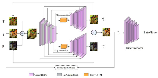
Figure 1. The framework of RABRRN. Where the symbol ⊕ denotes the feature stitching of the image. ⨂ denotes the combination of the transmitting and reflecting layers. For the encoder, the first Conv + ReLU block denotes layer 1 convolution, the second Conv + ReLU block denotes layers 2–3, the third Conv + ReLU block denotes layers 4–6, and the last Conv + ReLU block denotes the remaining convolution layers.

It is well known that attention exerts a remarkable impact in human perception. One of the most fundamental characteristics of the human visual system is that there is no need to process an entire scene at once. Instead, humans deliberately focus on some important sections of the image through a series of partial glimpses to better capture the visual structure. Therefore, we argue that reflection removal is an issue of spatial variational occlusion removal sensitive to both spatial and channel factors, rather than just a problem of basic picture layer separation.

CBAM is a type of attention mechanism that adaptively refines features in channel and space, which are two separated dimensions. Before the residual network [30] was proposed, the problem of vanishing gradient occurred as a result of increased depth in deep neural networks. The training set loss gradually lowers as the amount of network layers grows, and then the loss tends to become saturated. If the network depth increases continuously, the training loss will decline step by step. With the residual block (ResBlock) introduced, which is the fundamental block of the residual network, the neural network can reach a much greater depth, and the performance will also be better.

In this paper, we combined CBAM and ResNet into a residual attention network module (ResCbamBlock), which increases the depth of the network and enhances the channel and spatial representation, thus improving the feature extraction ability of the network. The structure of the ResCbamBlock is illustrated in Figure 2. The input of the ResCbamBlock is feature map x. Additionally, after two convolutions, the refined feature map x″ can be acquired from x. Then, in the channel attention block, two pooling operations (max-pooling and average-pooling) are added to x″ to extract two vectors. These two vectors are input into the shared network (SN), then merged with the output feature vectors using element-wise summation to obtain the channel attention map (Mc(x″)). The SN consists of a multi-layer perceptron (MLP) and a hidden layer. The feature map x′″ with enhanced channel features is obtained by multiplying Mc(x″) and x″ in an element-wise manner. Subsequently, in the spatial attention block, two pooling operations are used to generate two 2D maps representing the mean-pooling and max-pooling features of the entire channel, respectively. The two maps are connected with each other, and then, through a standard convolutional layer, a two-dimensional spatial attention map Ms(x″’) is generated. The element-wise multiplication of Ms(x″’) and x″’ is performed to obtain a feature map f with enhanced spatial features, and the final output of ResCbamBlock is f + x.

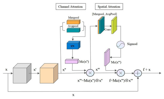
Figure 2. Structure of ResCbamBlock: a building block where the symbol ⊕ denotes the element-wise summation. ⨂ denotes the element-wise multiplication.

For discriminator networks, previous studies have experimentally demonstrated that discriminator networks of typical generative adversarial networks (GAN) [31] are, in many cases, not suitable for the domain of high-resolution, high-detail image recovery. Hence, we designed PatchGAN discriminators for the reflection removal recovery task. Differing from general networks in the discriminator, PatchGAN employs a Markov discriminator that effectively builds the image as a random Markov field to divide a pair of images into image blocks, assuming that the independence between pixels is greater than the size of the image blocks, as shown in Figure 3. In contrast to the discriminators in a typical GAN, the PatchGAN discriminator outputs a two-dimensional matrix instead of individual values. In simple terms, the output of a typical GAN discriminator is a single value of 0 or 1. This means that the discriminator looks at the entire image and determines whether the image is real or false. If the image is real, it should equal 1. If the image is fake, it should give 0. Typical GAN discriminators focus on the whole image and, therefore, may ignore the local texture details of the image. Each element of this matrix output by PatchGAN is between 0 and 1. Finally, a matrix corresponding to the discriminant result of the image block is output, and the discriminant result of the whole image is taken as the average of the discriminant results of all image blocks. It is worth noting that each element represents a local region in the input image, and the discriminator needs to view multiple local image blocks to determine the authenticity of each image block. By doing so, the local texture details of the generated image can be enhanced, further improving the visual quality of the generated image.

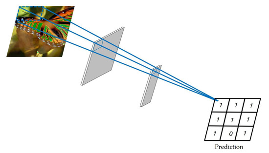
Figure 3. Our discriminator: the output is a two-dimensional matrix in which each element represents a local region of the input image, and the value of the matrix element is 1 if the local region is real and 0 otherwise.

Our discriminator network has six convolutional layers, and the first five convolutional layers use a strided convolution with a convolutional kernel size of 3 × 3 and a step size of 2. The first convolutional layer extracts 64 channels of features from the generated image, except for the fifth stride convolutional layer, where the dimensionality of the feature map is multiplied, while the other stride convolutional layers are down sampled. The last layer is a 1 × 1 convolution operation, which compresses all the feature dimension information into one channel dimension. After five stride convolution layers, the size of the feature map is 1/32 of the original input, so the whole process essentially outputs the original input image of a 256 × 256 size as an 8 × 8 matrix, and the final evaluation result of the whole image is taken as the average of the discriminant results of all image blocks.

In general, we avoided using traditional convolutional networks as sub-networks during the iterative training process, for those networks will make the training of the entire model difficult. In the RABRRN, we use two convolutional LSTM blocks, one for each decoder branch. ConvLSTM is from FC-LSTM [32], which uses the output of a fully connected neural network as the input of LSTM to achieve a better performance. If the time series data is an image, adding a convolution operation to LSTM can improve the capacity to capture the spatial characteristics of the image, which will be more effective than using LSTM only. As shown in Figure 4, the ConvLSTM module has four gates, including input gate i, forgetting gate f, output gate o, and unit state c. Input gate i controls how much information from the current computation is added to the cell state. Forgetting gate f determines how much of the information passed over from the previous iteration will be forgotten. Output gate o controls how much information from the current state will be passed to the next iteration. Unit state c controls the state after passing through the input gate and the forgetting gate, which determines the current state of a unit. In each iteration, the information from the previous step is saved and provided to the next step in the ConvLSTM, which can be used to solve the gradient elimination problem in recursive convolutional neural networks. The key equation of ConvLSTM is shown in Equation (1), where ∗ denotes the convolution operation, ∘ denotes the Hadamard product, and b represents the activation value of the cell.

$$\begin{gathered} i_t=\sigma \left(W_{xi}\ast x_t+W_{hi}\ast h_{t-1}+W_{ci}\circ c_{t-1}+b_i\right) \\ {f}_t=\sigma \left(W_{xf}\ast x_t+W_{hf}\ast h_{t-1}+W_{cf}\circ c_{t-1}+b_f\right) \\ {c}_t=f_t\circ c_{t-1}+i_t\circ tanh\left(W_{xc}\ast x_t+W_{hc}\ast h_{t-1}+b_c\right) \\ {o}_t=\sigma \left(W_{xo}\ast x_t+W_{ho}\ast h_{t-1}+W_{co}\circ c_t+b_o\right) \\ {h}_t=o_t\circ tanh\left(c_t\right) \end{gathered}$$

(1)

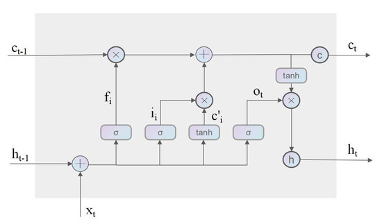
Figure 4. ConvLSTM structure.

As shown in Figure 1, the reflection removal network progressively refines the prediction results for the transmission and reflection layers through iterations. At the beginning of training, the I and T are initialized as the original reflection image I, and R is set to be a tensor of the same size as I, and the value of each pixel is set to 0.1 for the three RGB channels. In addition, the input to the network is a cascade of T, I, and R. The predicted values of the new transmission and reflection layers, $\underset{ }{\overset{^}{\mathrm{T}}}$ and $\underset{ }{\overset{^}{\mathrm{R}}}$, are then obtained by convolving two sub-networks of the LSTM utilized as inputs for the following time step, while information is memorized in the LSTM network for the prediction of the next time step. The predicted values of the transmission and reflection are reconstructed by the hybrid image formation model for the hybrid image $\underset{ }{\overset{^}{\mathrm{I}}}$. The reconstructed hybrid image is used to compare with the real input hybrid image to guide the output of the network; there are corresponding loss functions between the predicted transmission layer image and the real transmission layer image as well as between the predicted reflection image and the real reflection image. Finally, the result of the prediction network for the transmission layer at the final step n is the transmission layer’s final prediction result.

3.2. Loss Function

In this section, we present the loss functions utilized in the RABRRN network training. Let T and R be the ground truth of the transmission layer and reflection layer, respectively, and the predicted transmission layer and reflection layer at iteration t are denoted as ${\underset{ }{\overset{^}{\mathrm{T}}}}_{\mathrm{t}}$ and ${\underset{ }{\overset{^}{\mathrm{R}}}}_{\mathrm{t}}$, respectively.

Pixel Loss and Structural Similarity Loss: Pixel loss is used to penalize pixel-level differences between T and ${\underset{ }{\overset{^}{\mathrm{T}}}}_{\mathrm{t}}$. The objective is to reduce the error between the generated transmission layer and the ground truth. Since the L₁ loss has a stable gradient for whatever input value does not lead to the gradient explosion problem, we utilize the L₁ loss function to calculate the pixel loss as a more robust solution. Summing up the reasons, our pixel loss is summarized as:

$${ℒ}_{pixel}={\displaystyle \sum }_{\mathcal{T}\in \mathcal{D}}{\displaystyle \sum }_{t=1}^N{\mathsf{\theta }}^{\mathrm{N}-\mathrm{t}}{ℒ}_1\left({\mathrm{T}}_{,}{\underset{ }{\overset{^}{\mathrm{T}}}}_{\mathrm{t}}\right)$$

(2)

in which θ is defined at 0.85.

Zhao [33] proposed that in image restoration, the combination of SSIM (Structural Similarity Index Measure) [34] loss and L₁ loss is better than L₂ loss. Because of the computational simplicity, most of the previous research used only pixel loss, but it may lead to the generation of blurred images because it is different from the human visual perception of natural images. Therefore, to provide more natural visual results, we took the human visual perception of natural images into consideration when designing the loss function. In our reflection removal task, the SSIM is used to calculate the degree of similarity between the estimated T and ${\underset{ }{\overset{^}{\mathrm{T}}}}_{\mathrm{t}}$ and their associated ground truth. The SSIM is described as:

$$\mathrm{SSIM}(\mathrm{T},{\underset{ }{\overset{^}{\mathrm{T}}}}_{\mathrm{t}})=\frac{(2{\mathsf{\mu }}_{\mathrm{T}}{\mathsf{\mu }}_{{\underset{ }{\overset{^}{\mathrm{T}}}}_{\mathrm{t}}}+{\mathrm{C}}_1)(2{\mathsf{\sigma }}_{{\mathrm{T}\underset{ }{\overset{^}{\mathrm{T}}}}_{\mathrm{t}}}+{\mathrm{C}}_2)}{({\mathsf{\mu }}_{\mathrm{T}}^2+{\mathsf{\mu }}_{{\underset{ }{\overset{^}{\mathrm{T}}}}_{\mathrm{t}}}^2+{\mathrm{C}}_1)({\mathsf{\sigma }}_{\mathrm{T}}^2+{\mathsf{\sigma }}_{{\underset{ }{\overset{^}{\mathrm{T}}}}_{\mathrm{t}}}^2+{\mathrm{C}}_2)}$$

(3)

where ${\mathsf{\mu }}_{\mathrm{T}}$ and ${\mathsf{\mu }}_{{\underset{ }{\overset{^}{\mathrm{T}}}}_{\mathrm{t}}}$ are the means of $\mathrm{T}$ and ${\underset{ }{\overset{^}{\mathrm{T}}}}_{\mathrm{t}}$, ${\sigma }_{\mathrm{T}}$ and ${\sigma }_{{\underset{ }{\overset{^}{\mathrm{T}}}}_{\mathrm{t}}}$ are the variances in $\mathrm{T}$ and ${\underset{ }{\overset{^}{\mathrm{T}}}}_{\mathrm{t}}$, and ${\mathsf{\sigma }}_{{\mathrm{T}\underset{ }{\overset{^}{\mathrm{T}}}}_{\mathrm{t}}}$ is their corresponding covariances. SSIM measures the similarity between the real and generated images in three dimensions: contrast, luminance, and structure.

Therefore, similar to [27], which also adopts ${ℒ}_{\mathrm{t}}^{\mathrm{SSIM}}=1-\mathrm{SSIM}({\mathrm{T}}_{, }{\underset{ }{\overset{^}{\mathrm{T}}}}_{\mathrm{t}})$ as the loss term in each iteration t, the ${ℒ}_{\mathrm{SSIM}}$ used in this paper is formulated as:

$${ℒ}_{SSIM}={\displaystyle \sum }_{\mathcal{T}\in \mathcal{D}}{\displaystyle \sum }_{t=1}^N{\mathsf{\theta }}^{\mathrm{N}-\mathrm{t}}{ℒ}_{\mathrm{t}}^{\mathrm{SSIM}}$$

(4)

in which θ is defined at the same value as ${ℒ}_{pixel}$. The mixture of pixel loss and SSIM loss is defined as follows:

$${ℒ}_{mix}=\beta {ℒ}_{\mathrm{SSIM}}+\left(1-\beta \right){ℒ}_{pixel}$$

(5)

in which the β set value is 0.84 according to [33].

Adversarial Loss: Noticeably, MSE loss networks based on simple convolutional neural networks tend to produce images with unnatural and blurred backgrounds because the image generated with this loss function is the average of several natural solutions. In order to avoid this problem, Goodfellow proposed adversarial loss [31]. Adversarial loss is used to encourage the generative network to output images that match natural image distribution. The occurrence of color bias and blurred images is a common problem in reflection removal tasks. Therefore, in our approach, applying adversarial loss can better guide the generation of more natural images. The adversarial loss in our reflection removal task is defined as:

$${ℒ}_{adv}={\displaystyle \sum }_{\mathcal{T}\in \mathcal{D}}-\log D\left(\mathrm{T},\underset{ }{\overset{^}{\mathrm{T}}}\right)$$

(6)

Reconstruction Loss: For the predicted transmission and reflection layers, we generate reflection images using an image synthesis operation. Then, the reconstructed loss function is constructed from the composed picture and the original reflection image. The experimental results show that the reconstructed loss works well. The experimental results demonstrate that the rebuilt loss is effective. One possible explanation is that the two branch networks share the same network topology and have complementary goals. With the same network structure, they could be simultaneously either under-trained or over-trained, so the error of the reconstruction loss will be doubled if both sub-networks are in an under-trained or over-trained state. Therefore, the use of reconstruction loss in our task minimizes the error in both branch networks to ensure that the predicted reflection image (recombination of the transmission and reflection layers) is similar to the original input. We use the mean least squared error (MSE) to calculate the reconstruction loss, and the perceptual distance between the reconstructed image and the input image is defined as:

$${ℒ}_{res}={\displaystyle \sum }_{\mathcal{T}\in \mathcal{D}}{\displaystyle \sum }_{t=1}^N{ℒ}_{\mathrm{MSE}}\left(\mathrm{I},{\underset{ }{\overset{^}{\mathrm{I}}}}_{\mathrm{t}}\right)$$

(7)

Multi-scale Perceptual Loss: To extract features for perceptual loss, we utilize a pre-trained VGG-19 network [35]. The multi-scale perceptual loss collects features from multiple decoder levels and inputs them into convolution layers to generate outputs of various resolutions, and then the distance between the generated image and real image is calculated. We can gain additional contextual information from multiple layers of input by employing this loss in training. The loss function is defined as:

$${ℒ}_{MP}={\displaystyle \sum }_{{\mathcal{T}}^j\in \mathcal{D}}{\displaystyle \sum }_{j=1,3,5}^N{\mathsf{\gamma }}^{\mathrm{j}}{ℒ}_{VGG}\left(\mathrm{T},{\underset{ }{\overset{^}{\mathrm{T}}}}_{\mathrm{j}}\right)$$

(8)

where ${ℒ}_{\mathrm{VGG}}$ represents the loss between VGG features, ${\underset{ }{\overset{^}{\mathrm{T}}}}_{\mathrm{j}}$ represents the output of the last j layer at time step N, and ${\mathrm{T}}_{\mathrm{j}}$ represents the ground truth value at the same scale as ${\underset{ }{\overset{^}{\mathrm{T}}}}_{\mathrm{j}}$. We set γ¹=1, γ³=0.8, and γ⁵=0.6, respectively. In the VGG-19 network, we compare the features of the conv1_2 and conv2_2 layers.

Total Loss: In general, the total loss function for our network training is defined as:

$$ℒ={\mathsf{\lambda }}_1{ℒ}_{\mathrm{mix}}+{ \mathsf{\lambda }}_2{ℒ}_{\mathrm{adv}}+{ \mathsf{\lambda }}_3{ℒ}_{\mathrm{res}}+{ \mathsf{\lambda }}_4{ℒ}_{\mathrm{MP}}$$

(9)

Experimental results showed that mixture loss objective functions play a key role in obtaining high quality results. Therefore, the weights are set to 2. Reconstruction loss is beneficial in guiding the two sub-networks to work together, allowing the generation of visually better transmission images, so the weight parameter of the reconstruction loss function is also set to 2. In addition, the experimentally verified adversarial loss and perceptual loss are set to 0.25 and 0.1, respectively. Therefore, the weights of each loss in the experiment are set as follows: λ₁ = 2, λ₂ = 0.25, λ₃ = 2, and λ₄ = 0.01.

4. Experiments

In the experiments, we used the 64-bit Ubuntu16.04 operating system and the deep learning framework PyTorch1.2.0. The GPU-accelerated training was performed on a GeForce GTX 1080Ti with a graphics card memory of 32G, and the CUDA version was 10.2. To minimize the training loss, we employed the ADAM optimizer [36] to train our model for 90 epochs, where β₁ and β₂ in ADAM were both set to 0.5, the batch size was set to 2, and the learning rate for the whole network training was set to 0.0002. Too many training epochs do not provide better experimental results, and we chose to train 90 epochs based on our experiments.

Deep neural network training needs a significant amount of data; however, the available reflection datasets are limited. Therefore, we also collected more real reflection images. We utilized a stand to hold the camera and a piece of movable glass in front of the camera for taking photos. Images with reflections were obtained by setting the glass between the camera and the objects to be photographed. Images without reflections were also obtained by quickly removing the glass. In Figure 5, the device for taking pictures and two pictures with and without reflection are illustrated. We published the dataset we collected in the Data Availability Statement section of our paper.

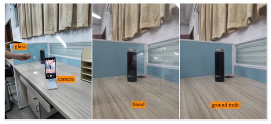
Figure 5. The method of SCAU-RID dataset collection and a pair of sample images.

As for the real data, we used 460 pairs of real images, which consisted of 250 pairs of real data from ERRNet [28], 110 pairs of real data from Zhang [1], and 100 pairs from the SCAU-RID dataset we collected. As for the synthetic data, we used the pictures dataset from [25] for the synthetic data, with 8000 pairs of synthetic images available for comparison (size: 512 × 512).

4.1. Quantitative Evaluation

To evaluate the performance of our method, we compared the model with RmNet [25], Zhang [1], ERRNet [28], and IBLCN [26] in terms of both quality and quantity. As reference standards, we also used the comparison of the hybrid image and the ground truth. We used the code and pre-trained model supplied by the authors in their team for a fair comparison and set the parameters as specified in their original publication. Meanwhile, we used PSNR (Peak Signal to Noise Ratio) [37], SSIM, and LMSE [38] as evaluation metrics. Only PSNR has units (dB) among these three evaluation metrics. PSNR is the most widely used image quality evaluation index, and it is based on the difference in error between corresponding pixels and error-sensitive image quality evaluation. The higher the value, the better the predicted image’s visual perception. Real natural images are highly structured, i.e., there are strong correlations between the pixels of the image, and these correlations carry information about the structure of the object. SSIM senses the distortion information of an image by detecting whether the structural information has changed, and measures the similarity of two images in terms of brightness, contrast, and structure. Regarding SSIM, the higher the SSIM value is, the better the overall image quality can be predicted too, and the overall image performance is closer to the ground truth. Meanwhile, LMSE represents the minimum mean square error of the output image and the real image, and a smaller value of LMSE implies a better result.

The findings of the competing approaches on the four real datasets are summarized in Table 1. The first row of the dataset is from the Nature test dataset of Li [26], and the remaining three rows are from the SIR² constructed by [39]; SIR² includes three sub-datasets: Object, Postcard and Wild. On the Nature and Wild datasets, our technique is clearly the best, second on the combined dataset of objects, and third on Postcard. In addition, to make the comparison of quantitative data acquired using different methods more intuitive, we visualized the data of PSNR and SSIM, as shown in Figure 6. This has validated that our method can achieve superior performance in various real-world scenarios.

Table 1. A quantitative comparison of three real-world benchmark datasets and three alternative techniques. The top result are highlighted in red, while the second best results are highlighted in blue.

Dataset	Index	Methods
		RmNet [25]	Zhang [1]	ERRNet [28]	IBLCN [26]	Ours
Nature [28]	PSNR	20.525	22.221	21.351	23.422	24.284
	SSIM	0.785	0.812	0.881	0.893	0.897
	LMSE	0.032	0.025	0.023	0.014	0.021
Object [39]	PSNR	21.347	22.032	23.565	23.375	23.622
	SSIM	0.772	0.802	0.874	0.868	0.859
	LMSE	0.031	0.030	0.023	0.019	0.021
Postcard [39]	PSNR	22.125	21.415	23.637	23.601	23.521
	SSIM	0.847	0.797	0.862	0.876	0.871
	LMSE	0.027	0.024	0.017	0.014	0.019
Wild [39]	PSNR	21.576	21.051	23.153	23.675	23.721
	SSIM	0.794	0.820	0.862	0.869	0.883
	LMSE	0.029	0.027	0.025	0.018	0.016

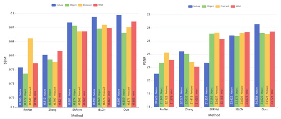
Figure 6. Data visualization of evaluation metrics PSNR and SSIM for qualitative comparisons, where the x-axis displays various methods and the y-axis reflects the values, and the different colored bars in the same method represent the results on different datasets.

4.2. Qualitative Evaluation

To further compare different algorithms through visual evaluation, we present some test results in Figure 7 and Figure 8, where each column represents the input of the image, the result of the method comparison, and the ground truth, respectively. The first and second rows in Figure 7 are from the Nature dataset, the third to fifth rows are from ERRNet-50, and the last two rows are in our collected SCAU-RID dataset. The seven types of pictures are toys, indoor potted plants, tripods, houses, pavilions, trees, and outdoor potted plants. The three rows in Figure 8 are from three sub-datasets of the SIR² dataset using pictures of bridges, stationery, and toys. To make the evaluation more intuitive, some local patches with strong reflection signals are marked with yellow rectangles in the input image.

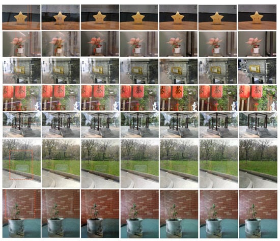
Figure 7. Qualitative comparison between the proposed method and four state-of-the-art techniques. The images are obtained from ‘Nature’ (Rows 1–2), ‘ERRNet-50’ (Rows 3–5), and our SCAU-RID (Rows 6–7). In particular, the first column represents the input image, the last column represents the ground truth image without reflections, and the other columns represent the output corresponding to the comparison method. Column 2 from RmNet [25], column 3 from Zhang [1], column 4 from ERRNet [28], column 5 from IBLCN [26] and column 6 from ours work.

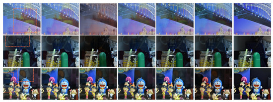
Figure 8. Qualitative comparison between the proposed method and four state-of-the-art techniques. The images are obtained from ‘SIR²’ (Rows 1–3). In particular, the first column represents the input image, the last column represents the ground truth image without reflections, and the other columns represent the out-put corresponding to the comparison method. Column 2 from RmNet [25], column 3 from Zhang [1], column 4 from ERRNet [28], column 5 from IBLCN [26] and column 6 from ours work.

From the first 2 rows in Figure 7, it can be seen that our method had a good performance in an indoor environment, and the reflection created by incandescent lamps in indoor potted plants was well removed. RmNet performed poorly, even worse than the input results. Zhang’s method darkened the restored background as a whole. As seen in the third and fifth rows, none of the methods for comparison can completely remove large-area reflections and strong reflections. IBCLN performed the best on the third row but suffered from color distortion and significant reflection artifacts. By contrast, our method was effective, although it enlarged the original black spots. The reflection of houses in the fourth row was not very strong, and both our method and IBLCN obtained a near-perfect removal effect. For large-area reflections from pavilions, only ERRNet could achieve desirable outcomes. At the same time, in the last two rows in Figure 7, we also listed the test results on our SCAU-RID dataset. It can be observed that our method could remove reflections more effectively while recovering clearer high-frequency details of the background image, although there were also some reflection artifacts.

As can be seen in Figure 8, the structure of the reflected church in the first row of the bridge image is clear, indicating that our method has a good visual effect, with the majority of the reflective layers properly removed while avoiding color distortion. In addition, it is obvious that Zhang’s method caused serious chromatic aberrations. However, for the stationery in the second row, as the high and low-frequency information was not obvious, the reflection was mistaken for the background information in all methods, resulting in a poor performance in reflection removal. In the third row, ERRNet and our method performed better despite a few residual reflections in the image of toys. By contrast, RmNet and Zhang are ineffective.

To better evaluate the performance of the proposed method comprehensively, we show in Figure A1 in the Appendix A the experimental results of our method on a larger number of samples.

4.3. Ablation Study

We ran an ablation study by altering the model components, removing or replacing the loss function, and retraining the network to better assess our network design and evaluate the loss function. In particular, we used the full Equation (9) for the ablation analysis of the network structure. We analyzed the loss function using the complete network structure as in Figure 1. We conducted three comparative experiments, respectively, deleting ResCbamBlock, using CBAM to replace ResCbamBlock, and replacing the mixed loss with pixel loss and the same network structure. PSNR and SSIM were obtained by evaluating the retrained models in these experiments, and the experimental results of the ablation study are shown in Table 2. Compared with using CBAM alone, using ResCbamBlock improved the PSNR score by 1.406 dB and the SSIM score by 0.052. Removing ResCbamBlock reduced PSNR by 2.930 dB and SSIM by 0.087. Compared with using pixel loss alone, the hybrid function of pixel loss and structural similarity loss improved PSNR by 0.587 dB and SSIM by 0.064 without changing the network structure.

Table 2. A quantitative comparison of various network architectures and loss function approaches was performed. The best outcomes are highlighted in red, while the second best results are highlighted in blue.

Method	PSNR	SSIM	LSME
Del ResCbamBlock	21.578	0.816	0.032
ResCbamBlock → CBAM	23.102	0.852	0.027
$ℒ$mix → $ℒ$pixel	23.493	0.839	0.24
Complete	24.284	0.897	0.021

In addition, we analyzed the parameters of different models, as shown in Table 3. The RABRRN achieved better removal results with parameters of only 18.524M, which was one third of the RmNet parameters.

Table 3. The comparison of parameter quantity between our method, RmNet [25], and IBLCN [26], indicating that our method has fewer parameters. The best outcomes are highlighted in red, while the second best results are highlighted in blue.

Method	Parameter	PSNR	SSIM
RmNet [25]	65.443M	21.393	0.779
IBLCN [26]	21.608M	23.518	0.876
Ours	18.524M	23.787	0.885

5. Conclusions

In this study, we proposed an RABRRN based on a residual attention mechanism for single image reflection removal. It is a dual-streamline architecture composed of one encoder and two decoders with identical structures, with two branches used to predict the transmission layer and the reflection layer, respectively. To improve the quality of predictions, we introduced a residual attention module in the encoder, which brings a superior removal effect as shown from experimental data. For the network model training, we combined pixel loss and structural similarity loss in order to produce results consistent with human perception. Furthermore, we established a reflection image dataset named SCAU-RID to study image reflection removal. By comparing our method with the state-of-art, the quantitative and qualitative results revealed that the single image reflection removal method proposed in this paper significantly improved the quality of restored images while reducing the number of parameters.

There is a lack of a general framework in the field of image restoration, and the existing models are developed and designed for specific tasks. In the near future, we aim to apply the improved network to other image processing tasks such as rain removal, haze removal, and shadow removal. Although we have achieved desirable results in our experiment, it seems that we could not achieve good results for strong reflections over large areas, and we will carry out more research on eliminating large and strong reflections afterwards.

References

- Zhang, X.; Ng, R.; Chen, Q. Single image reflection separation with perceptual losses. In Proceedings of the IEEE Conference on Computer Vision and Pattern Recognition, Salt Lake City, UT, USA, 18–23 June 2018; pp. 4786–4794. [Google Scholar]
- Li, Y.; Brown, M.S. Single image layer separation using relative smoothness. In Proceedings of the IEEE Conference on Computer Vision and Pattern Recognition, Columbus, OH, USA, 23–28 June 2014; pp. 2752–2759. [Google Scholar]
- Shih, Y.C.; Krishnan, D.; Durand, F.; Freeman, W.T. Reflection removal using ghosting cues. In Proceedings of the IEEE Conference on Computer Vision and Pattern Recognition, Boston, MA, USA, 7–12 June 2015; pp. 3193–3201. [Google Scholar]
- Lei, C.; Chen, Q. Robust reflection removal with reflection-free flash-only cues. In Proceedings of the IEEE/CVF Conference on Computer Vision and Pattern Recognition, Nashville, TN, USA, 20–25 June 2021; pp. 14811–14820. [Google Scholar]
- Xingjian, S.H.I.; Chen, Z.; Wang, H.; Yeung, D.Y.; Wong, W.K.; Woo, W.C. Convolutional LSTM network: A machine learning approach for precipitation nowcasting. In Advances in Neural Information Processing Systems; MIT Press: Cambridge, MA, USA, 2015; pp. 802–810. [Google Scholar]
- Sun, C.; Liu, S.; Yang, T.; Zeng, B.; Wang, Z.; Liu, G. Automatic reflection removal using gradient intensity and motion cues. In Proceedings of the 24th ACM International Conference on Multimedia, Amsterdam, The Netherlands, 15–19 October 2016; pp. 466–470. [Google Scholar]
- Szeliski, R.; Avidan, S.; Anandan, P. Layer extraction from multiple images containing reflections and transparency. In Proceedings of the IEEE Conference on Computer Vision and Pattern Recognition, CVPR 2000 (Cat. No. PR00662). Hilton Head, SC, USA, 15 June 2000; Volume 1, pp. 246–253. [Google Scholar]
- Gai, K.; Shi, Z.; Zhang, C. Blind separation of superimposed moving images using image statistics. IEEE Trans. Pattern Anal. Mach. Intell. 2011, 34, 19–32. [Google Scholar]
- Guo, X.; Cao, X.; Ma, Y. Robust separation of reflection from multiple images. In Proceedings of the IEEE Conference on Computer Vision and Pattern Recognition, Columbus, OH, USA, 23–28 June 2014; pp. 2187–2194. [Google Scholar]
- Nandoriya, A.; Elgharib, M.; Kim, C.; Hefeeda, M.; Matusik, W. Video reflection removal through spatio-temporal optimization. In Proceedings of the IEEE International Conference on Computer Vision, Venice, Italy, 22–29 October 2017; pp. 2411–2419. [Google Scholar]
- Sinha, S.N.; Kopf, J.; Goesele, M.; Scharstein, D.; Szeliski, R. Image-based rendering for scenes with reflections. ACM Trans. Graph. (TOG) 2012, 31, 1–10. [Google Scholar] [CrossRef]
- Lei, C.; Huang, X.; Zhang, M.; Yan, Q.; Sun, W.; Chen, Q. Polarized reflection removal with perfect alignment in the wild. In Proceedings of the IEEE/CVF Conference on Computer Vision and Pattern Recognition, Seattle, WA, USA, 13–19 June 2020; pp. 1750–1758. [Google Scholar]
- Simon, C.; Kyu Park, I. Reflection removal for in-vehicle black box videos. In Proceedings of the IEEE Conference on Computer Vision and Pattern Recognition, Boston, MA, USA, 7–12 June 2015; pp. 4231–4239. [Google Scholar]
- Kong, N.; Tai, Y.W.; Shin, J.S. A physically-based approach to reflection separation: From physical modeling to constrained optimization. IEEE Trans. Pattern Anal. Mach. Intell. 2013, 36, 209–221. [Google Scholar] [CrossRef] [PubMed]
- Wolff, L.B. Polarization-based material classification from specular reflection. IEEE Trans. Pattern Anal. Mach. Intell. 1990, 12, 1059–1071. [Google Scholar] [CrossRef]
- Levin, A.; Zomet, A.; Weiss, Y. Learning to perceive transparency from the statistics of natural scenes. In Advances in Neural Information Processing Systems; MIT Press: Cambridge, MA, USA, 2002; Volume 15. [Google Scholar]
- Levin, A.; Zomet, A.; Weiss, Y. Separating reflections from a single image using local features. In Proceedings of the 2004 IEEE Computer Society Conference on Computer Vision and Pattern Recognition, CVPR 2004, Washington, DC, USA, 27 June–2 July 2004; Volume 1. [Google Scholar]
- Levin, A.; Weiss, Y. User assisted separation of reflections from a single image using a sparsityprior. IEEE Trans. Pattern Anal. Mach. Intell. 2007, 29, 1647–1654. [Google Scholar] [CrossRef] [PubMed]
- Wan, R.; Shi, B.; Hwee, T.A.; Kot, A.C. Depth of field guided reflection removal. In Proceedings of the 2016 IEEE International Conference on Image Processing (ICIP), IEEE, Phoenix, AZ, USA, 25–28 September 2016; pp. 21–25. [Google Scholar]
- Arvanitopoulos, N.; Achanta, R.; Susstrunk, S. Single image reflection suppression. In Proceedings of the IEEE Conference on Computer Vision and Pattern Recognition, Honolulu, HI, USA, 21–26 July 2017; pp. 4498–4506. [Google Scholar]
- Fan, Q.; Yang, J.; Hua, G.; Chen, B.; Wipf, D. A generic deep architecture for single image reflection removal and image smoothing. In Proceedings of the IEEE International Conference on Computer Vision, Venice, Italy, 22–29 October 2017; pp. 3238–3247. [Google Scholar]
- Chi, Z.; Wu, X.; Shu, X.; Gu, J. Single image reflection removal using deep encoder-decoder network. arXiv preprint 2018, arXiv:1802.00094. [Google Scholar]
- Wan, R.; Shi, B.; Duan, L.Y.; Tan, A.-H.; Kot, A.C. Crrn: Multi-scale guided concurrent reflection removal network. In Proceedings of the IEEE Conference on Computer Vision and Pattern Recognition, Salt Lake City, UT, USA, 18–23 June 2018; pp. 4777–4785. [Google Scholar]
- Wan, R.; Shi, B.; Li, H.; Duan, L.-Y.; Tan, A.-H.; Kot, A.C. CoRRN: Cooperative reflection removal network. IEEE Trans. Pattern Anal. Mach. Intell. 2019, 42, 2969–2982. [Google Scholar] [CrossRef] [PubMed]
- Wen, Q.; Tan, Y.; Qin, J.; Liu, W.; Han, G.; He, S. Single image reflection removal beyond linearity. In Proceedings of the IEEE/CVF Conference on Computer Vision and Pattern Recognition, Long Beach, CA, USA, 15–20 June 2019; pp. 3771–3779. [Google Scholar]
- Li, C.; Yang, Y.; He, K.; Lin, S.; Hopcroft, J.E. Single image reflection removal through cascaded refinement. In Proceedings of the IEEE/CVF Conference on Computer Vision and Pattern Recognition, Seattle, WA, USA, 13–19 June 2020; pp. 3565–3574. [Google Scholar]
- Dong, Z.; Xu, K.; Yang, Y.; Xu, W.; Lau, R.W. Location-aware single image reflection removal. In Proceedings of the IEEE/CVF International Conference on Computer Vision, Montreal, QC, Canada, 10–17 October 2021; pp. 5017–5026. [Google Scholar]
- Wei, K.; Yang, J.; Fu, Y.; Wipf, D.; Huang, H. Single image reflection removal exploiting misaligned training data and network enhancements. In Proceedings of the IEEE/CVF Conference on Computer Vision and Pattern Recognition, Long Beach, CA, USA, 15–20 June 2019; pp. 8178–8187. [Google Scholar]
- Woo, S.; Park, J.; Lee, J.Y.; Kweon, I.S. Cbam: Convolutional block attention module. In Proceedings of the European conference on computer vision (ECCV), Munich, Germany, 8–14 September 2018; pp. 3–19. [Google Scholar]
- He, K.; Zhang, X.; Ren, S.; Sun, J. Deep residual learning for image recognition. In Proceedings of the IEEE conference on computer vision and pattern recognition, Las Vegas, NV, USA, 27–30 June 2016; pp. 770–778. [Google Scholar]
- Goodfellow, I.; Pouget-Abadie, J.; Mirza, M.; Xu, B.; Warde-Farley, D.; Ozair, C.; Courville, A.; Bengio, Y. Generative adversarial networks. Commun. ACM 2020, 63, 139–144. [Google Scholar] [CrossRef]
- Srivastava, N.; Mansimov, E.; Salakhudinov, R. Unsupervised learning of video representations using lstms. In Proceedings of the International Conference on Machine Learning, PMLR, Lille, France, 6–11 July 2015; pp. 843–852. [Google Scholar]
- Zhao, H.; Gallo, O.; Frosio, I.; Kautz, J. Loss functions for neural networks for image processing. arXiv preprint 2015, arXiv:1511.08861. [Google Scholar]
- Wang, Z.; Bovik, A.C.; Sheikh, H.R.; Simoncelli, E.P. Image quality assessment: From error visibility to structural similarity. IEEE Trans. Image Process. 2004, 13, 600–612. [Google Scholar] [CrossRef] [PubMed]
- Simonyan, K.; Zisserman, A. Very deep convolutional networks for large-scale image recognition. arXiv preprint 2014, arXiv:1409.1556. [Google Scholar]
- Kingma, D.P.; Ba, J. Adam: A method for stochastic optimization. arXiv preprint 2014, arXiv:1412.6980. [Google Scholar]
- Avcibas, I.; Sankur, B.; Sayood, K. Statistical evaluation of image quality measures. J. Electron. Imaging 2002, 11, 206–223. [Google Scholar]
- Grosse, R.; Johnson, M.K.; Adelson, E.H.; Freeman, W.T. Ground truth dataset and baseline evaluations for intrinsic image algorithms. In Proceedings of the 2009 IEEE 12th International Conference on Computer Vision, IEEE, Kyoto, Japan, 29 October–2 November 2009; pp. 2335–2342. [Google Scholar]
- Wan, R.; Shi, B.; Duan, L.Y.; Tan, A.-H.; Kot, A.C. Benchmarking single-image reflection removal algorithms. In Proceedings of the IEEE International Conference on Computer Vision, Venice, Italy, 22–29 October 2017; pp. 3922–3930. [Google Scholar]
Disclaimer/Publisher’s Note: The statements, opinions and data contained in all publications are solely those of the individual author(s) and contributor(s) and not of MDPI and/or the editor(s). MDPI and/or the editor(s) disclaim responsibility for any injury to people or property resulting from any ideas, methods, instructions or products referred to in the content. |
© 2023 by the authors. Licensee MDPI, Basel, Switzerland. This article is an open access article distributed under the terms and conditions of the Creative Commons Attribution (CC BY) license (https://creativecommons.org/licenses/by/4.0/).