Fault Detection Algorithm Based on Dynamic Global–Local Preserving Projection

Abstract

Industrial system operations usually have dynamic characteristics. If these characteristics are ignored, the performance of fault detection degrades. Herein, the fault-detection algorithm of dynamic global–local preserving projection (DGLPP) is employed to solve the problem mentioned. First, time-delay data are added to the sample to form an augmentation matrix and characterize the system dynamics. Second, the dimensionality of the augmented matrix is reduced using global–local preserving projection. The dimensionality-reduction method can preserve the data’s global and local structures. Then, a DGLPP model is built using the dimensionality-reduced data. Moreover, Hotelling’s T² and squared prediction error (SPE) statistics are used for fault detection. Finally, this method is used to detect the fault in the Tennessee Eastman (TE) process. The experimental results show that the DGLPP method has an enhanced fault detection rate. Moreover, the fault-detection effects of the DGLPP method are better than those of the principal component analysis (PCA), local preserving projection (LPP), and global–local preserving projection (GLPP) methods.

1. Introduction

The rapid development of big data, artificial intelligence, and other technologies and the integration of informatization and automation have made industrial processes increasingly complex and highly integrated. All links of a complex system are closely connected. Even a minor failure may cause a major security accident. Therefore, fault-detection technology is crucial in modern industrial processes. In recent years, deep-learning methods have achieved great success in fault diagnosis. However, their practical applications still have some challenges. Deep-learning methods typically require large amounts of labeled data for training. However, large-scale labeled data may be difficult to obtain in the field of fault diagnosis. In addition, deep-learning models are barely explanatory; thus, explaining why a particular fault diagnosis result is produced can be difficult. The artificial neural network has also made some progress in the field of fault diagnosis. However, the artificial neural network also has some limitations and shortcomings in fault diagnosis. The construction of the neural network model consumes a lot of time and cost. Secondly, the network model requires high-quality sample data, while the acquisition and processing of sample data may be limited in the actual situation. In addition, the complexity and size of the network model increases with the increase in the sample data and may not be suitable for large systems. The data-driven fault-detection method can analyze and mine the feature relationship between data to build a monitoring model. This method is often used for system fault detection because of its data-driven nature. Many industrial-process data can be collected and preserved by extensively applying distributed control systems. This scenario creates conditions for data-driven, fault-diagnosis methods [1,2,3,4,5]. Classic data-driven methods include PCA [6,7,8,9], fisher discriminant analysis (FDA) [10], partial least squares [11,12,13], and independent PCA [14,15,16]. These methods have been widely used in process monitoring and fault detection for industrial systems. However, these algorithms maintain only the data’s global structure while ignoring the local features of the data. Stream-learning methods represented by LPP [17,18,19] and neighborhood preserving embedding (NPE) [20,21,22] have been developed and widely used in recent years. These methods can extract hidden intrinsic properties from high-dimensional data and maintain their local structural features. They preserve the data’s local structure by constructing the neighborhood connection graph. However, these methods ignore the data’s global structure. They can project the data only into a very narrow area; in particular, they cannot project the data with a non-neighbor relationship to a very long distance. Therefore, these methods have certain limitations.

Neither PCA nor LPP can consider data’s global and local structures. Therefore, the important features of the data cannot be fully represented in the low-dimensional space using these methods. In response to this problem, Zhang M. et al. proposed a fault-detection method for global–local structure analysis by constructing a double-objective function, combining the characteristics of PCA and LPP [23]. On the basis of similar ideas, Yu et al. proposed local and global PCA [24]. In this method, a double-objective function based on LPP and PCA was constructed using the ratio for the simultaneous extraction of global and local features. Luo L. et al. proposed an algorithm called GLPP [25]. This method successfully unifies global and local structures in the same framework. Luo L.J. et al. proposed a nonlocal and local structure-preserving projection algorithm for fault detection [26]. Nonlocal and local similarity weight coefficients are utilized in this method to control the distance between the projected data points. Thus, the data’s nonlocal and local structures are preserved. Ma designed a local and nonlocal embedding algorithm based on NPE [27]. In this algorithm, the original spatial data structure is extracted by minimizing the nearest neighbor sample distance and maximizing the nonlocal sample distance. Tang combined FDA with GLPP to minimize intraclass scattering and maximize interclass scattering [28]. This method preserves the global and local structures of the data. It also ensures the discriminability of the shadow-casting space and improves fault detection performance. The above methods have achieved satisfactory results in process monitoring. However, they still have limitations for systems with dynamic characteristics.

Moreover, data in industrial processes are dynamic. It is closely related to a number of factors such as time, operational control, external conditions, and production materials and processes. And, it is updated and changed using these factors. The dynamic nature of this data is essential for the monitoring, control, and optimization of the production process. Therefore, the dynamic process modeling and monitoring method of mining temporal features has been given considerable attention. Aiming at the system’s dynamic characteristics, Ku W. et al. proposed a dynamic PCA (DPCA) method [29]. The delayed measurement values are introduced to form an augmented matrix, which is then modeled via PCA. Zhang C. et al. proposed a fault detection and diagnosis method based on DPCA residual heterogeneity by combining DPCA and mutual heterogeneity methods [30]. This method can reduce the adverse influence of dynamic characteristics on fault detection. Xu J. et al. used a sliding window approach to expand the original matrix into a dynamic matrix [31]. This dynamic matrix can effectively characterize the autocorrelation property of time series. Miao A M. et al. used a time series extended-NPE algorithm to establish an information-extraction strategy based on a space and time structure [32]. The dynamic correlation of data with time is obtained by learning the characteristics of time-series data. Li Y. et al. proposed a method termed time–space nearest neighborhood standardization [33]. The dynamic characteristics of the data are eliminated by locating and standardizing the samples’ local neighbors in time and space.

A fault-detection algorithm based on DGLPP is proposed in this study to solve the low efficiency of system fault detection using dynamic characteristics. The system’s dynamic characteristics are extracted by adding time-delay data to an augmented matrix. The global–local holding projection is used to reduce the dimension and preserve the data’s global–local structure. Then, the DGLPP model is constructed, and the corresponding T² and SPE statistics are established for fault detection. Finally, the proposed algorithm is applied to the fault detection of the TE process to evaluate its effectiveness. Experimental results show that this algorithm has a higher fault-detection rate than PCA, LPP, and GLPP algorithms. This algorithm effectively captures the dynamic characteristics of the system and preserves the data’s relevant structural features. It also improves fault-detection performance and contributes to the dynamic system fault-detection research.

This article is organized as follows. In Section 1, the background and research status of the topic are described. Then, the algorithms related to fault diagnosis are introduced in Section 2. In Section 3, the algorithms used in this study are described in detail. The main idea of this study is discussed in Section 4. The proposed algorithm is applied to the TE process for fault detection, and the results are analyzed. Section 5 presents the conclusions of this study.

2. Background Techniques

2.1. PCA Algorithm

The basic idea of PCA involves retaining most of the maximum variance information via orthogonal transformations to ensure that the data loses the least information after dimensionality reduction [34,35,36]. The aim is to include as much information as possible about most changes in the original dataset with minimal combined data. In particular, a set of mapping matrices $P=(p_1,p_2\cdots p_l)$ is found for a given dataset $X=(x_1,x_2\cdots x_n)\in R^{n\times m}$ and projected onto a low-dimensional space to obtain a mapping matrix $Y=(y_1,y_2\cdots y_n)$. Its objective function is as follows:

$$\begin{array}{l}{J}_{Global}=\underset{p}{\max }{{\displaystyle \sum _{i=1}^n(y_i-\overline{y})}}^2\\ subjectto:p^{T}p=1\end{array}$$

(1)

where $\overline{y}=\frac{1}{n}{\displaystyle \sum _{i=1}^n{y}_i}$. The dataset $X\in R^{n\times m}$ ($m$ is the number of variables in the sample and $n$ is the number of samples) is decomposed by PCA into the following:

$$X=X_p+E=T{P}^T+E$$

(2)

where $X_p$ is the projection of the sample vector $X$ in the principal element subspace, $T$ is the score matrix, $P$ is the load matrix, and $E$ is the residual subspace.

2.2. LPP Algorithm

The LPP method is a linear approximation of the Laplacian feature map for extracting features from the data while preserving the local manifold information of the data [37,38]. For the initial dataset $X$, a transformation matrix $W$ is calculated and projected into a low-dimensional space to obtain the dataset $Y$ after dimensionality reduction. The objective function is as follows:

$$\begin{array}{l}{J}_{LPP}={\underset{a}{\min }}^2{{\displaystyle \sum _{ij}(y_i-y_j)}}^2{W}_{ij}\\ subjectto:a^{T}XD{X}^{T}a=1\end{array}$$

(3)

where the diagonal matrix $D(d_{ii}={\displaystyle \sum _j{w}_{ij})}$ represents the distance between sample points. The larger the value of $d_{ii}$ is, the more important the corresponding point $y_i$ is. The weight matrix $W$ represents the distance relationship between the sample points in the dataset. Its size can be calculated using the kernel function, as shown in Equation (4).

$${\mathrm{W}}_{ij}=\left\{\begin{array}{ll}{e}^{-\frac{‖x_i-x_j‖}{t}}& if{x}_j\in {\Psi }_k(x_i)or{x}_i\in {\Psi }_k(x_j)\\ 0& otherwise\end{array}\right.$$

(4)

where $t$ is the parameter of the heat kernel function. Its value range is $5m{\sigma }^2\le t\le 10m{\sigma }^2$($m$ is the number of sample variables and $\sigma$ is the sample variance). The appropriate values from this range are derived based on manual experience. ${\Psi }_k(x_i)$ is the set of the first $k$-nearest neighbors of the sample.

3. Fault Detection Based on DGLPP

3.1. Dynamic Characterization

The data in industrial processes are dynamic, and a time series autocorrelation exists between process variables. The autocorrelation between sample points can be characterized well by extending the original matrix into a dynamic matrix. Therefore, the first l-time delay samples can be introduced to construct the augmentation vector of the samples at the current time.

$$X_k(l)=\left[X(k) X(k-1) \cdots X(k-l)\right]$$

(5)

where $X(k-l)$ is the $m$ dimensional variable at time $k-l$ and $l$ is the delay length.

3.2. DGLPP Algorithm

After establishing the augmented matrix to obtain the dynamic information of the system, the GLPP method is used to reduce the dimension of the data and the DGLPP model is established for fault detection.

The idea of GLPP involves combining the local structure preserving objective function and the global variance maximum objective function to construct the local and global preserving objective function. As a result, the dimensionality-reduced data retain the global structure and local nearest neighbor structure of their original feature space. In particular, the original high-dimensional dataset $X$ is mapped to the low-dimensional space by transforming matrix $A$ to obtain the reduced-dimension dataset $Y$ and ensure that the generated dataset $Y$ can fully retain the global and local structures of the original dataset $X$. The objective function for constructing GLPP is shown as follows:

$$\underset{a}{\min }\{J_{Lobal}(a),J_{Glocal}(a)\}$$

(6)

where $a$ is the transformation vector. Moreover, the subfunction $J_{Local}(a)=\frac{1}{2}{\displaystyle {\sum }_{ij}{(y_i-y_j)}^2{W}_{ij}}$ stores the local structure of the data, and the subfunction $J_{Glocal}(a)=-\frac{1}{2}{\displaystyle {\sum }_{ij}{(y_i-y_j)}^2}\stackrel{\Lambda }{W_{ij}}$ stores the global structure of the data. $W_{ij}$ is the adjacency weight matrix, representing the adjacency of $x_i$ and $x_j$. Any pair of adjacent points $x_i$ and $x_j$ in space has a corresponding nonzero $W_{ij}$. The calculation formula of $W_{ij}$ is shown as follows:

$${\mathrm{W}}_{ij}=\left\{\begin{array}{ll}{e}^{-\frac{‖x_i-x_j‖}{\sigma }}& if{x}_j\in {\Omega }_k(x_i)or{x}_i\in {\Omega }_k(x_j)\\ 0& otherwise\end{array}\right.$$

(7)

where $\sigma$ is the empirical constant and ${\Omega }_k(x_i)$ is the first $k$-nearest neighbor set of the $x_i$ sample. Unlike $W_{ij}$, $\stackrel{\wedge }{W_{ij}}$ is a non-neighborhood weight matrix. $\stackrel{\wedge }{W_{ij}}$ represents the non-neighborhood of $x_i$ and $x_j$. Any pair of non-neighboring points $x_i$ and $x_j$ in space has a corresponding nonzero $\stackrel{\wedge }{W_{ij}}$. The formula for $\stackrel{\wedge }{W_{ij}}$ is as follows:

$$\stackrel{\wedge }{W_{ij}}=\left\{\begin{array}{ll}{e}^{\frac{{}^{-‖x_i-x_j‖}}{\sigma }}& if{x}_j\notin {\Omega }_k(x_i)and{x}_i\notin {\Omega }_k(x_j)\\ 0& otherwise\end{array}\right.$$

(8)

The subobjective function $J_{Local}(a)=\frac{1}{2}{\displaystyle {\sum }_{ij}{(y_i-y_j)}^2{W}_{ij}}$ is further transformed into the following:

$$\begin{array}{ll}\hfill J_{Local}(a)& =\frac{1}{2}{\displaystyle \sum _{ij}{(y_i-y_j)}^2{W}_{ij}}\hfill \\ & ={\displaystyle \sum _{ij}{y}_i{D}_{ii}{y}_i{}^T}-{\displaystyle \sum _{ij}{y}_i{W}_{ij}{y}_j{}^T}\hfill \\ & ={\displaystyle \sum _{ij}{a}^T{x}_i{D}_{ii}{x}_i^{T}a}-{\displaystyle \sum _{ij}{a}^T{x}_i{W}_{ij}{x}_j^{T}a}\hfill \\ & =a^{T}X(D-W)X^{T}a\hfill \\ & =a^{T}XL{X}^{T}a\hfill \end{array}$$

(9)

where $L=D-W$ is the Laplace matrix, $D$ is the diagonal matrix, and the diagonal element $D_{ii}={\displaystyle {\sum }_j{W}_{ij}}$ is the sum of the elements of the corresponding rows or columns of the nearest neighbor weight matrix $W$. Similarly, the subobjective function $J_{Glocal}(a)=-\frac{1}{2}{\displaystyle {\sum }_{ij}{(y_i-y_j)}^2}\stackrel{\Lambda }{W_{ij}}$ can be rewritten as follows:

$$\begin{array}{ll}\hfill J_{Glocal}(a)& =-\frac{1}{2}{\displaystyle \sum _{ij}{(y_i-y_j)}^2}\stackrel{\Lambda }{W_{ij}}\hfill \\ & =-{\displaystyle \sum _{ij}{y}_i{\stackrel{\Lambda }{D}}_{ii}{y}_i{}^T}-{\displaystyle \sum _{ij}{y}_i\stackrel{\Lambda }{W_{ij}}{y}_j{}^T}\hfill \\ & =-{\displaystyle \sum _{ij}{a}^T{x}_i{\stackrel{\Lambda }{D}}_{ii}{x}_i^{T}a}-{\displaystyle \sum _{ij}{a}^T{x}_i\stackrel{\Lambda }{W_{ij}}{x}_j^{T}a}\hfill \\ & =-a^{T}X(\stackrel{\Lambda }{D}-\stackrel{\Lambda }{W})X^{T}a\hfill \\ & =-a^{T}X\stackrel{\Lambda }{L}{X}^{T}a\hfill \end{array}$$

(10)

where $\stackrel{\Lambda }{L}=\stackrel{\Lambda }{D}-\stackrel{\Lambda }{W}$ is the Laplace matrix, $\stackrel{\Lambda }{D}$ is the diagonal matrix, and ${\stackrel{\Lambda }{D}}_{ii}={\displaystyle {\sum }_j{\stackrel{\Lambda }{W}}_{ij}}$.

GLPP introduces a weighting coefficient $\eta$ to optimize the global and local features’ subobjective functions simultaneously. The bio-objective optimization can be transformed into the following single-objective optimization problem by using this weighting coefficient:

$$\begin{array}{ll}\hfill J_{GLPP}(a)& =\underset{a}{\min \frac{1}{2}}\{\eta J_{Lobal}(a)+(1-\eta )J_{Glocal}(a)\}\hfill \\ & =\underset{a}{\min }\frac{1}{2}\{\eta {\displaystyle {\sum }_{ij}{(y_i-y_j)}^2{W}_{ij}}-(1-\eta ){\displaystyle {\sum }_{ij}{(y_i-y_j)}^2\stackrel{\wedge }{W_{ij}}}\}\hfill \\ & =\underset{a}{\min }\frac{1}{2}{\displaystyle {\sum }_{ij}{(y_i-y_j)}^2{R}_{ij}}\hfill \end{array}$$

(11)

where $\eta \in [0,1]$ is determined using the spectral radius $\rho (L)$ and $\rho (\stackrel{\wedge }{L})$ of the matrices $L$ and $\stackrel{\wedge }{L}$ corresponding to the global and local manifold structure, as follows:

$$\eta =\frac{\rho (\stackrel{\wedge }{L})}{\rho (L)+\rho (\stackrel{\wedge }{L})}.$$

(12)

Different tradeoff parameters $\eta$ correspond to different degrees of preservation and extraction of local and global manifold structure information. After the weight coefficient $\eta$ is determined, the $R_{ij}$ in Equation (11) is also obtained. Equation (13) can be further simplified using algebraic transformation as follows:

$$\begin{array}{ll}\hfill J_{GLPP}(a)& =\underset{a}{\min }\frac{1}{2}{\displaystyle {\sum }_{ij}{(y_i-y_j)}^2{R}_{ij}}\hfill \\ & =\underset{a}{\min }\{{\displaystyle \sum _i{y}_i}{H}_{ii}{y}_i^T-{\displaystyle {\sum }_{ij}{y}_i{R}_{ij}{y}_i^T}\}\hfill \\ & =\underset{a}{\min }\{{\displaystyle \sum _i{a}^T{x}_i}{H}_{ii}{x}_i^{T}a-{\displaystyle {\sum }_{ij}{a}^T{x}_i{R}_{ij}{x}_i^{T}a}\}\hfill \\ & =\underset{a}{\min }{a}^{T}X(H-R)X^{T}a\hfill \\ & =\min a^{T}XM{X}^{T}a\hfill \end{array}$$

(13)

where $M=H-R$ is the Laplace matrix, $H$ is the diagonal matrix, and $H_{ii}={\displaystyle {\sum }_i{R}_{ii}}$.

The objective function of GLPP is constrained as follows:

$$a^T(\eta XH{X}^T+(1-\eta )I)a^T=a^{T}Na=1$$

(14)

GLPP solves the following transformation problems to find the optimal transformation vector:

$$\begin{array}{l}\underset{\overrightarrow{a}}{\min }{a}^{T}XM{X}^{T}a\\ s.t.a^{T}Na=1\end{array}$$

(15)

where $N=\eta XH{X}^T+(1-\eta )I$,$H=\eta D-(1-\eta )\stackrel{\wedge }{D}$ and $I$ is the identity matrix. Therefore, the optimal transformation vector $A$ can be obtained by solving the problem of generalized eigenvectors $a$:

$$XM{X}^{T}a=\lambda Na.$$

(16)

The eigenvalues obtained from the solution are sorted from smallest to largest ${\lambda }_1<{\lambda }_2\cdots {\lambda }_l$. Their corresponding eigenvectors are the obtained projection matrix $A$ that can maintain the global and local structures of the data, which can be constructed as:

$$x_i\to y_i=A^T{x}_i=[a_1,a_2\cdots a_l].$$

(17)

3.3. Indicators for Monitoring Statistics

DGLPP utilizes Hotelling’s T² and SPE statistics as the detection indicators of the model. The system operates normally when the $T^2$ statistic is lower than the control limit $T_{\alpha }$; otherwise, a failure occurs:

$$T_i^2=y^T{S}^{-1}y<T_{\alpha }$$

(18)

where $S$ is the covariance matrix of matrix y after the dimensionality reduction of the training set sample $S=\frac{1}{n-1}{Y}^{T}Y$.

$T_{\alpha }$ is calculated using the following formula:

$$T_{\alpha }=\frac{\alpha (n+1)(n-1)}{n(n-\alpha )}{F}_{\alpha }(\alpha ,n-\alpha )$$

(19)

where $\alpha$ is the test level and $F_a\left(a,n-a\right)$ is the $F$ distribution with $\alpha$ as the first degree of freedom and $n-\alpha$ as the second degree of freedom.

The system operates normally when the $SPE$ statistic is below the control limit $Q_{\alpha }$; otherwise, a failure occurs:

$$SPE={‖x-Ay‖}^2<Q_{\alpha }.$$

(20)

$Q_{\alpha }$ is calculated as follows:

$$Q_{\alpha }={\theta }_1{(\frac{c_{\alpha }{h}_0\sqrt{2{\theta }_2}}{{\theta }_1}+1+\frac{{\theta }_2{h}_0(h_0-1)}{{\theta }_1^2})}^{1/h_0}$$

(21)

where ${\theta }_i={\displaystyle \sum _{j=k+1}^m{\lambda }_j^i}(i=1,2,3)$, $h_0=1-2{\theta }_1{\theta }_3/3{\theta }_1^2$, and $c_a$ is the confidence limit of the standard normal distribution.

In addition, to ensure the reliability of T² and SPE, we need to regularly update $T_{\alpha }$ and $Q_{\alpha }$. This enables adaptation to changes in data distribution, variable correlation, fault modes, timely detect, and correct model drift. It also ensures the accuracy and reliability of the fault detection model.

3.4. DGLPP Fault Detection Process

The flowchart of using DGLPP for fault detection is shown in Figure 1. The process is mainly divided into two steps: offline modeling and online diagnosis. The specific steps are as follows.

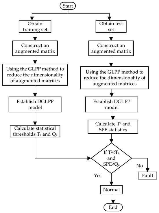
Figure 1. Fault detection flow char.

Offline modeling:

• Collect the system’s historical data under normal working conditions as the training set samples.
• Construct an augmentation matrix for each sample in the training set.
• Use the GLPP algorithm to reduce the augmented matrix’s dimensionality and establish the DGLPP model.
• Calculate the statistical threshold $T_{\alpha }$ and $Q_{\alpha }$ for the DGLPP model.

Online diagnosis:

• Obtain system online data as test set samples.
• Construct an augmentation matrix for each sample in the test set.
• Use the GLPP algorithm to reduce the augmented matrix’s dimensionality and establish the DGLPP model.
• Calculate the T² and the SPE statistics for each sample in the test set.
• Determine whether the sample’s T² and the SPE statistics exceed their statistical thresholds. If so, the system fails; otherwise, the system operates normally.

4. TE Process Fault Detection

TE process is a simulation process based on a complex chemical reaction process simulation. Figure 2 shows a flow sheet of the TE process. TE processes are now used in many fields, such as control, optimization, and process monitoring. The TE process has become the most widely used benchmark test platform for monitoring performance evaluation in the field of process monitoring [39,40]. The process comprises five main units: reactor, compressor, condenser, gas–liquid separator, and product-refining tower. The TE process data used in this experiment include training datasets and 21 test datasets. The training dataset is sampled under normal conditions. It is also used for offline modeling of the monitoring method. The test set samples with faults are obtained during 48 h of running simulation and faults are introduced at 8 h. A total of 960 observation values are collected, with the first 160 observation values being normal data and the last 800 samples being fault data. The 21 types of faults are classified into six types. Table 1 describes the fault data types. Each dataset has 52 variables, consisting of 11 control variables and 41 measurement variables. The measurement variable comprises the process measurement variable and component measurement variable. Table 2 provides detailed descriptions of control variables and process measurement variables.

Figure 2. TE process flowchart.

Table 1. TE process fault description.

No.	Fault Description	Type
1	A/C feed ratio, component B unchanged (stream 4)	Step
2	Component B, A/C feed ratio unchanged (stream 4)	Step
3	Material D temperature (stream 2)	Step
4	Reactor cooling water inlet temperature	Step
5	Condenser cooling inlet temperature	Step
6	Material A feed loss	Step
7	Material C pressure loss	Step
8	A, B, C composition	Random variable
9	Material D feed temperature	Random variable
10	Material C temperature	Random variable
11	Reactor cooling water inlet temperature	Random variable
12	Condenser cooling water inlet temperature	Random variable
13	Reaction kinetics parameters	Slow drift
14	Reactor cooling water valve	Sticky
15	Condenser cooling valve	Sticky
16	Unknown	Unknown
17	Unknown	Unknown
18	Unknown	Unknown
19	Unknown	Unknown
20	Unknown	Unknown
21	Logistics 4 valve position	Constant position

Table 2. Variables of the TE process.

No.	Variable Description	No.	Variable Description
1	Material D feed amount	22	Separator grade
2	Material E feed amount	23	Separator pressure
3	Material A feed amount	24	Separator bottom flow (Flow 10)
4	Material A and C feed amount	25	Stripper grade
5	Compressor recirculation valve	26	Stripper pressure
6	Discharge valve	27	Stripper bottom flow (Flow 11)
7	Liquid flow of separator tank	28	Separator temperature
8	Stripper liquid product flow	29	Separator grade
9	Stripper flow valve	30	Changes in Material C temperature
10	Reactor cooling water valve	31	Stripper temperature
11	Condenser cooling water flow	32	Stripper flow rate
12	Material A feed (Flow 1)	33	Compressor power
13	Material D feed (Flow 2)	34	Reactor cooling water outlet temperature
14	Material E feed (Flow 3)	35	Separator cooling water outlet temperature
15	Total feed (Flow 4)	36	Stripper temperature
16	Recirculation flow (Flow 8)	37	Stripper flow rate
17	Reactor feed rate (Flow 6)	38	Compressor power
18	Reactor pressure	39	Reactor cooling water outlet temperature
19	Reactor class	40	Separator cooling water outlet temperature
20	Reactor temperature	41	Separator cooling water outlet temperature
21	Discharge rate (Stream 9)

PCA, LPP, GLPP, and DGLPP methods are used for fault detection to verify the proposed method’s effectiveness. The confidence level is 99%, the cumulative contribution rate is 85%, the delay is 1, and the number of neighbors is 5. The fault detection rates of 21 faults using the above methods are shown in Table 3. As shown in Table 3, the fault detection performance of the DGLPP method is superior to the fault detection performances of the other methods. Thus, the effectiveness of the proposed algorithm is verified. The DGLPP algorithm can detect all faults except faults 3, 9, and 15, indicating that the algorithm has a high fault coverage.

Table 3. Test set fault detection rate (%).

No.	PCA		LPP		GLPP		DGLPP
	T2	SPE	T2	SPE	T2	SPE	T2	SPE
1	98.75	99.12	99.88	98.88	99.75	98.75	99.88	98.62
2	98.0	98.5	98.88	98.25	98.88	97.50	99.12	97
3	0.63	7.25	8.62	0	10.37	0	18.62	0
4	0.37	29.13	99.88	0	100	0	100	0
5	22.13	30.38	100	21.12	100	18.25	100	13.38
6	98.25	100	100	100	100	100	100	100
7	33.75	100	100	61.25	100	32.37	100	27.25
8	92.13	96.75	98.25	94.87	98.25	92.25	98.38	73.88
9	1.0	6.12	7.62	0.13	8.13	0	14.87	0
10	18.62	36.75	91.13	16.38	91.25	2.13	93.5	0
11	3	34.63	76.12	0.63	80.13	0.13	87.75	0
12	90.25	93.63	99.88	90.75	99.88	76.5	100	51
13	92.25	92.5	95.63	91.63	95.63	89.12	96.37	85.25
14	0.13	71.88	100	10.50	100	0.25	100	0
15	1.75	9.0	17.87	0.25	19	0	28.75	0
16	8.13	34.88	93.75	6.25	94.5	0.37	96.63	0
17	4.62	40.25	95.63	11	96.63	3.87	97.88	0
18	87.88	88.5	90.87	87.75	91.37	87.5	92.13	85.12
19	0.13	7.25	87.75	0	93.13	0	99.12	0
20	4.62	40.25	90.75	13.75	91.13	4.5	91.75	0
21	12.63	40.62	61.12	15.62	64.88	4.75	59.5	0
MFDR	36.62	55.11	81.60	39	82.52	33.73	84.49	30.07

MFDR: mean fault detection rate.

Fault 15 is viscous, and the process variable is described as condensate cooling water valve failure. Figure 3 shows the process monitoring diagrams for all methods of Fault 15. As the figure shows, PCA and LPP algorithms can hardly detect faults in this case, and the detection effect of the GLPP algorithm is not ideal. This scenario occurs because this fault is weak, and the measured variables are slightly affected. The changes in the mean, variance, or peak time are difficult to observe. The DGLPP algorithm is sensitive to faults and can detect faults continuously. The DGLPP algorithm can detect faults earlier and relatively higher detection rate than the other algorithms.

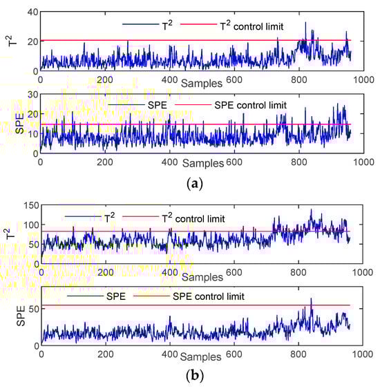
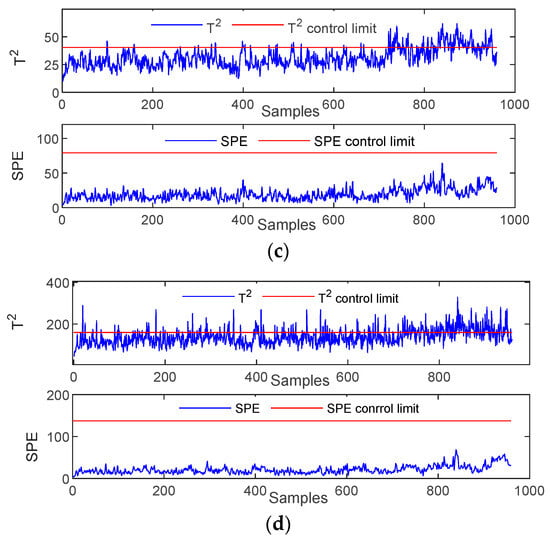
Figure 3. Monitoring charts for Fault 15: (a) PCA; (b) LPP; (c) GLPP; (d) DGLPP.

In the case where Fault 2 is the example, the feed flow ratio of A/C is constant; however, the content of component B changes step by step. This phenomenon causes the total feed to change. Thus, the system is prevented from operating normally, and a failure occurs. Four methods are used to detect this fault. The detection results are shown in Figure 4. All four methods can detect faults and realize continuous alarms. However, their fault detection sensitivities are nonidentical. PCA, LPP, GLPP, and DGLPP start to detect faults at 176, 171, 169, and 165 sample points, respectively. The test results demonstrate that the DGLPP method can detect the fault early, indicating that it has the best detection capability. The fault detection capability of the GLPP method is superior to the fault detection capabilities of the PCA and LPP methods. The reason is that GLPP considers the global and local features of the data in the modeling process and realizes a comprehensive feature extraction of the training data under normal conditions. Thus, its fault detection ability is improved. The DGLPP method further considers the dynamic characteristics of the data based on the GLPP method, and the data characteristics are retained accurately, further improving the detection performance.

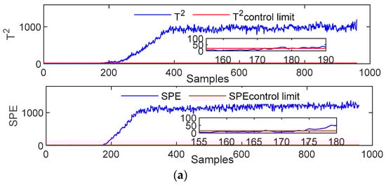
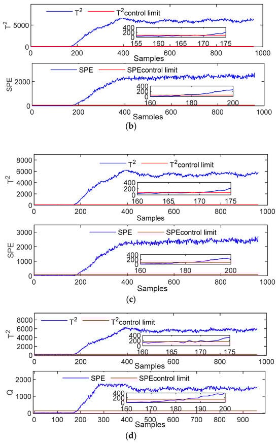
Figure 4. Monitoring charts for Fault 2: (a) PCA; (b) LPP; (c) GLPP; (d) DGLPP.

Fault 10 is a random disturbance in the feed temperature of Material C. This disturbance causes fluctuations in the feed temperature of Material C, resulting in a fault. The effect of fault detection is shown in Figure 5. When both T² and SPE statistics do not exceed the limit, it indicates that the system is operating normally at this time. Otherwise, it will cause a malfunction. Therefore, as shown in Figure 5, the PCA method can only detect a small number of faults. The SPE statistics of the LPP, GLPP, and DGLPP methods can hardly detect the faults, whereas the T² statistics can detect most of the faults. This is because there is a fault between process variables, and the relevant measurement coefficients between them remain stable. This caused a significant jump in the T² index value, while the SPE index remained within the threshold range with relatively small changes. However, these three methods also have underreporting in the subsequent detection process. DGLPP has relatively fewer missed sample points than the LPP and GLPP methods. With sample points 510–550 as the example, LPP, GLPP, and DGLPP miss 22, 21, and 19 sample points, respectively. Therefore, DGLPP has less under-reporting and higher detection accuracy than LPP and GLPP.

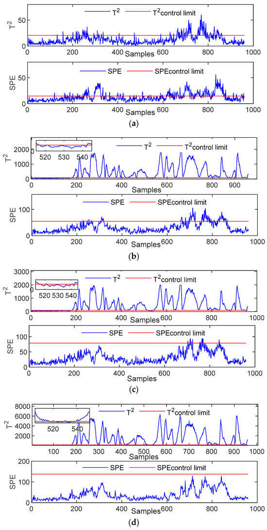
Figure 5. Monitoring charts for Fault 10: (a) PCA; (b) LPP; (c) GLPP; and (d) DGLPP.

5. Conclusions

A DGLPP fault detection algorithm is proposed to solve dynamic problems in industrial systems. An augmented matrix is obtained by adding time-delay data to characterize the system’s dynamic characteristics. Then, GLPP, which is more comprehensive and effective than other algorithms in extracting the feature information, is used to reduce the augmented matrix’s dimension to the low-dimensional space. Therefore, the DGLPP algorithm possesses remarkable detection effects. The TE example shows that the fault detection effect of the proposed method is more effective than the fault detection effects of PCA, LPP, and DGLPP, verifying the effectiveness of the proposed method.

References

- Mirnaghi, M.S.; Haghighat, F. Fault detection and diagnosis of large-scale HVAC systems in buildings using data-driven methods: A comprehensive review. Energy Build. 2020, 229, 110492. [Google Scholar] [CrossRef]
- Ge, Z. Review on data-driven modeling and monitoring for plant-wide industrial processes. Chemom. Intell. Lab. Syst. 2017, 171, 16–25. [Google Scholar] [CrossRef]
- Reis, M.S.; Gins, G. Industrial process monitoring in the big data/industry 4.0 era: From detection, to diagnosis, to prognosis. Processes 2017, 5, 35. [Google Scholar] [CrossRef]
- Wilhelm, Y.; Reimann, P.; Gauchel, W.; Mitschang, B. Overview on hybrid approaches to fault detection and diagnosis: Combining data-driven, physics-based and knowledge-based models. Procedia Cirp 2021, 99, 278–283. [Google Scholar] [CrossRef]
- Zhu, J.; Fan, C.; Yang, M.; Qian, F.; Mahalec, V. Data-driven models of crude distillation units for production planning and for operations monitoring. Comput. Chem. Eng. 2023, 177, 108322. [Google Scholar] [CrossRef]
- Yang, X.; He, R.; Wang, J.; Li, X.; Liu, R. Using thermal load matching strategy to locate historical benchmark data for moving-window PCA based fault detection in air handling units. Sustain. Energy Technol. Assess. 2022, 52, 102238. [Google Scholar] [CrossRef]
- Osornio-Rios, R.A.; Jaen-Cuellar, A.Y.; Alvarado-Hernandez, A.I.; Zamudio-Ramirez, I.; Cruz-Albarran, I.A.; Antonino-Daviu, J.A. Fault detection and classification in kinematic chains by means of PCA extraction-reduction of features from thermographic images. Measurement 2022, 197, 111340. [Google Scholar] [CrossRef]
- Ren, M.; Liang, Y.; Chen, J.; Xu, X.; Cheng, L. Fault detection for NOx emission process in thermal power plants using SIP-PCA. ISA Trans. 2023, 140, 46–54. [Google Scholar] [CrossRef]
- Lv, Z.; Yan, X.; Jiang, Q. Batch process monitoring based on multiple-phase online sorting principal component analysis. ISA Trans. 2016, 64, 342–352. [Google Scholar] [CrossRef]
- Nor, N.M.; Hussain, M.A.; Hassan, C.R.C. Fault diagnosis and classification framework using multi-scale classification based on kernel Fisher discriminant analysis for chemical process system. Appl. Soft Comput. 2017, 61, 959–972. [Google Scholar] [CrossRef]
- Yang, J.; Lv, Z.; Shi, H.; Tan, S. Performance monitoring method based on balanced partial least square and statistics pattern analysis. ISA Trans. 2018, 81, 121–131. [Google Scholar] [CrossRef]
- Harkat, M.F.; Mansouri, M.; Nounou, M.N.; Nounou, H.N. Fault detection of uncertain chemical processes using interval partial least squares-based generalized likelihood ratio test. Inf. Sci. 2019, 490, 265–284. [Google Scholar]
- Fazai, R.; Mansouri, M.; Abodayeh, K.; Nounou, H.; Nounou, M. Online reduced kernel PLS combined with GLRT for fault detection in chemical systems. Process Saf. Environ. Prot. 2019, 128, 228–243. [Google Scholar] [CrossRef]
- Sarath, R. Combined classification models for bearing fault diagnosis with improved ICA and MFCC feature set. Adv. Eng. Softw. 2022, 173, 103249. [Google Scholar]
- Gao, L.; Li, D.; Liu, X.; Liu, G. Enhanced chiller faults detection and isolation method based on independent component analysis and k-nearest neighbors classifier. Build. Environ. 2022, 216, 109010. [Google Scholar] [CrossRef]
- Wang, G.; Jin, S.; Zhao, G.; Zhao, J.; Xie, J. An independent component analysis based correlation coefficient method for internal short-circuit fault diagnosis of battery-powered intelligent transportation systems. Control Eng. Pract. 2023, 138, 105606. [Google Scholar] [CrossRef]
- Yu, Y.; Peng, M.J.; Wang, H.; Ma, Z.G.; Li, W. Improved PCA model for multiple fault detection, isolation and reconstruction of sensors in nuclear power plant. Ann. Nucl. Energy 2020, 148, 107662. [Google Scholar] [CrossRef]
- Shah, M.Z.H.; Hu, L.; Ahmed, Z. Modified LPP based on Riemannian metric for feature extraction and fault detection. Measurement 2022, 193, 110923. [Google Scholar] [CrossRef]
- Lin, X.; Sun, R.; Wang, Y. Improved key performance indicator-partial least squares method for nonlinear process fault detection based on just-in-time learning. J. Frankl. Inst. 2023, 360, 1–17. [Google Scholar] [CrossRef]
- Mou, M.; Zhao, X. Incipient fault detection and diagnosis of nonlinear industrial process with missing data. J. Taiwan Inst. Chem. Eng. 2022, 132, 104115. [Google Scholar] [CrossRef]
- Peng, K.; Guo, Y. Fault detection and quantitative assessment method for process industry based on feature fusion. Measurement 2022, 197, 111267. [Google Scholar] [CrossRef]
- Chen, H.; Wu, J.; Jiang, B.; Chen, W. A modified neighborhood preserving embedding-based incipient fault detection with applications to small-scale cyber–physical systems. ISA Trans. 2020, 104, 175–183. [Google Scholar] [CrossRef] [PubMed]
- Zhang, M.; Ge, Z.; Song, Z.; Fu, R. Global–local structure analysis model and its application for fault detection and identification. Ind. Eng. Chem. Res. 2011, 50, 6837–6848. [Google Scholar] [CrossRef]
- Yu, J. Local and global principal component analysis for process monitoring. J. Process Control 2012, 22, 1358–1373. [Google Scholar] [CrossRef]
- Luo, L. Process monitoring with global-local preserving projections. Ind. Eng. Chem. Res. 2014, 53, 7696–7705. [Google Scholar] [CrossRef]
- Luo, L.; Bao, S.; Mao, J.; Tang, D. Nonlocal and local structure preserving projection and its application to fault detection. Chemom. Intell. Lab. Syst. 2016, 157, 177–188. [Google Scholar] [CrossRef]
- Ma, Y.; Song, B.; Shi, H.; Yang, Y. Fault detection via local and nonlocal embedding. Chem. Eng. Res. Des. Trans. Inst. Chem. Eng. 2015, 94, 538–548. [Google Scholar] [CrossRef]
- Tang, Q.; Chai, Y.; Qu, J.; Fang, X. Industrial process monitoring based on Fisher discriminant global-local preserving projection. J. Process Control 2019, 81, 76–86. [Google Scholar] [CrossRef]
- Ku, W.; Storer, R.H.; Georgakis, C. Disturbance detection and isolation by dynamic principal component analysis. Chemom. Intell. Lab. Syst. 1995, 30, 179–196. [Google Scholar] [CrossRef]
- Zhang, C.; Dai, X.; Li, Y. Fault detection and diagnosis based on residual dissimilarity in dynamic principal component analysis. Acta Autom. Sin. 2022, 48, 292–301. [Google Scholar]
- Xu, J.; Wang, Z.L.; Wang, X. Fault detection for chemical process based on nonlinear dynamic global-local preserving projections. J. Chem. Eng. 2020, 71, 5655–5663. [Google Scholar]
- Miao, A.M.; Ge, Z.Q.; Song, Z.H.; Jiang, L.; Zhou, L. Neighborhood preserving embedding based on temporal extension and its application in fault detection. J. East China Univ. Sci. Technol. (Nat. Sci. Ed.) 2014, 40, 218–224. [Google Scholar]
- Li, Y.; Geng, Y.; Feng, L.W. Complex multi-stage process fault detection based on TSNS and KNN rules. Chem. Autom. Instrum. 2022, 49, 20–26. [Google Scholar]
- Yang, X.; Chen, J.; Gu, X.; He, R.; Wang, J. Sensitivity analysis of scalable data on three PCA related fault detection methods considering data window and thermal load matching strategies. Expert Syst. Appl. 2023, 234, 121024. [Google Scholar] [CrossRef]
- Wu, Y.; Liu, X.; Wang, Y.L.; Li, Q.; Guo, Z.; Jiang, Y. Improved deep PCA and Kullback–Leibler divergence based incipient fault detection and isolation of high-speed railway traction devices. Sustain. Energy Technol. Assess. 2023, 57, 103208. [Google Scholar] [CrossRef]
- Nawaz, M.; Maulud, A.S.; Zabiri, H.; Taqvi, S.A.A.; Idris, A. Improved process monitoring using the CUSUM and EWMA-based multiscale PCA fault detection framework. Chin. J. Chem. Eng. 2021, 29, 253–265. [Google Scholar] [CrossRef]
- Lu, N.; Li, M.; Zhang, G.; Li, R.; Zhou, T.; Su, C. Fault feature extraction method for rotating machinery based on a CEEMDAN-LPP algorithm and synthetic maximum index. Measurement 2022, 189, 110636. [Google Scholar] [CrossRef]
- Zhang, M.Q.; Kumar, A.; Chiu, M.S.; Luo, X.L. Non-convex logarithm embedding subspace weighted graph approach to fault detection with missing measurements. Neurocomputing 2022, 476, 87–101. [Google Scholar] [CrossRef]
- Lyman, P.R.; Georgakis, C. Plant-wide control of the Tennessee Eastman problem. Comput. Chem. Eng. 1995, 19, 321–331. [Google Scholar] [CrossRef]
- Downs, J.J.; Vogel, E.F. A plant-wide industrial process control problem. Comput. Chem. Eng. 1993, 17, 245–255. [Google Scholar] [CrossRef]
Disclaimer/Publisher’s Note: The statements, opinions and data contained in all publications are solely those of the individual author(s) and contributor(s) and not of MDPI and/or the editor(s). MDPI and/or the editor(s) disclaim responsibility for any injury to people or property resulting from any ideas, methods, instructions or products referred to in the content. |
© 2023 by the authors. Licensee MDPI, Basel, Switzerland. This article is an open access article distributed under the terms and conditions of the Creative Commons Attribution (CC BY) license (https://creativecommons.org/licenses/by/4.0/).