
MFFNet: A Building Extraction Network for Multi-Source High-Resolution Remote Sensing Data


Abstract
:1. Introduction
2. Related Work
2.1. Development of DCNNs
2.2. DCNN in the Remote Sensing Domain
- (i)
- Employing skip connections to link the encoder and decoder modules of the network, effectively merging global and local features.
- (ii)
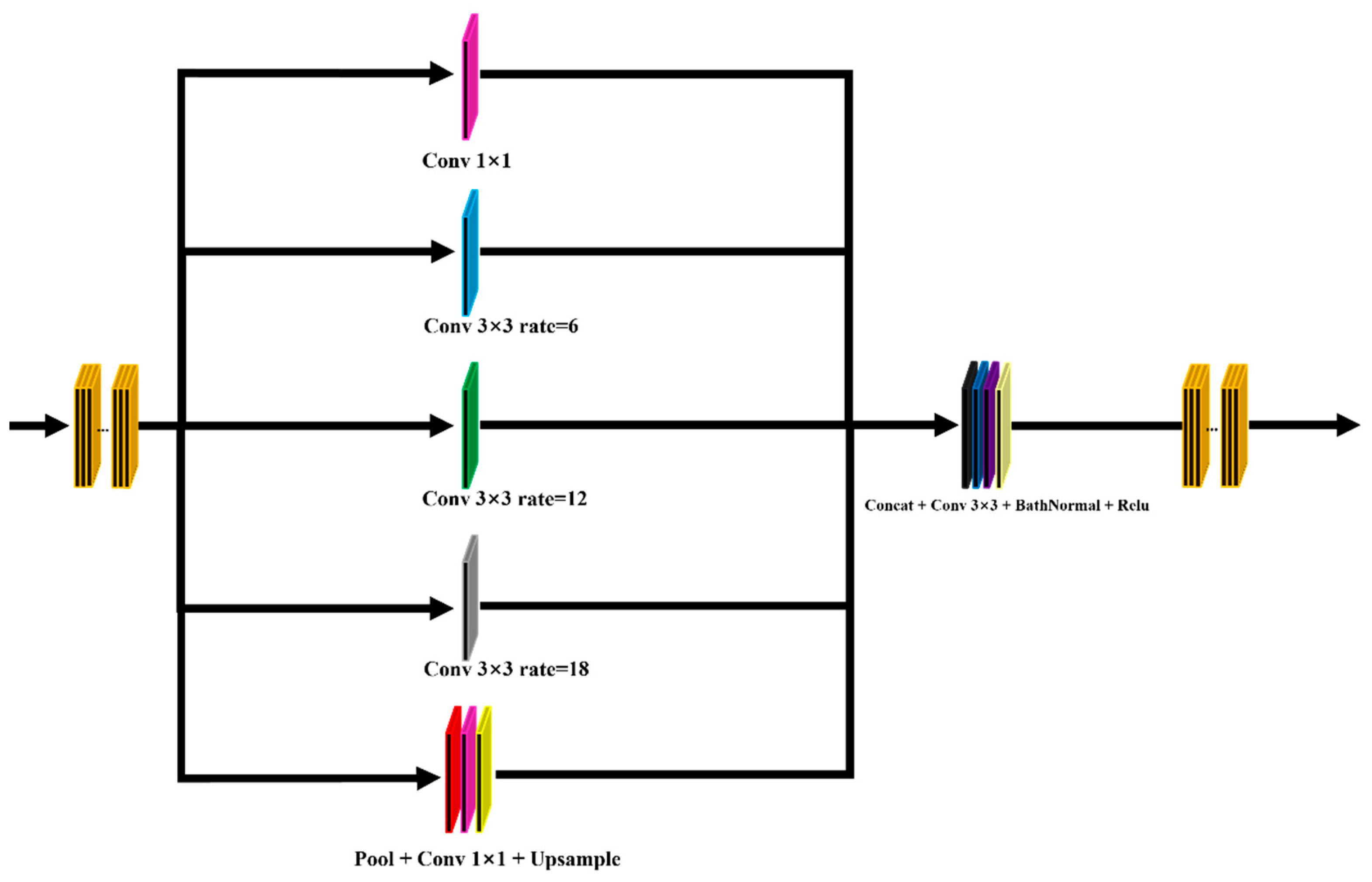
- Adopting the spatial pyramid approach, capturing semantic information of different scales through receptive fields of varying sizes, as seen in modules such as ASPP (atrous spatial pyramid pooling) and SPP (spatial pyramid pooling).
- (iii)
- Integrating attention mechanisms, allowing the network to fuse information across multiple scales.
- (iv)
- Enhancing the model using multi-level cascading methods. However, this is achieved under the cascade of various networks and does not necessarily indicate an enhancement in the segmentation accuracy of a single network.
2.3. Datasets
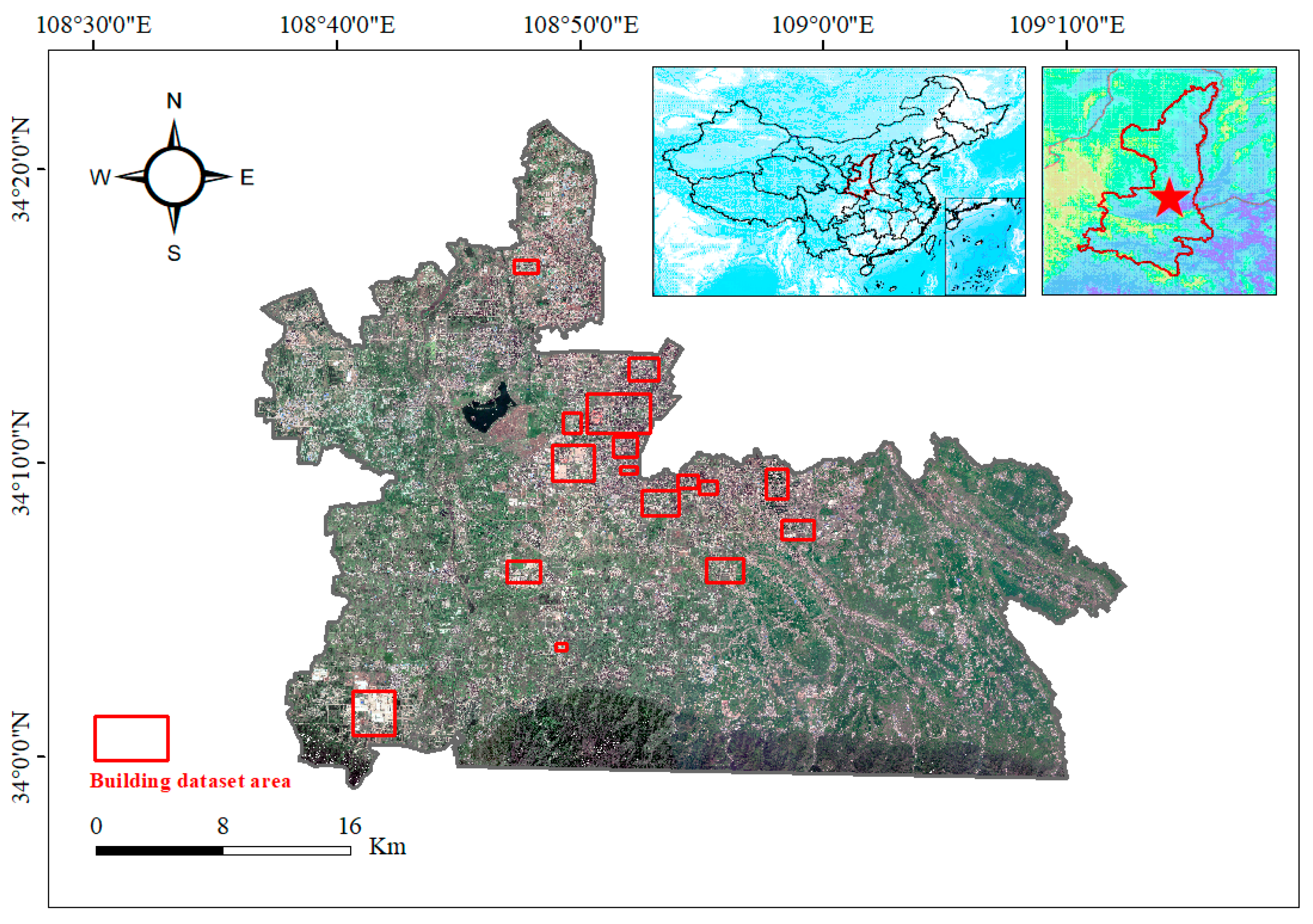
2.3.1. Jilin-1 Dataset
2.3.2. Massachusetts Building Dataset
2.3.3. WHU Building Dataset
3. Model and Evaluation Metrics
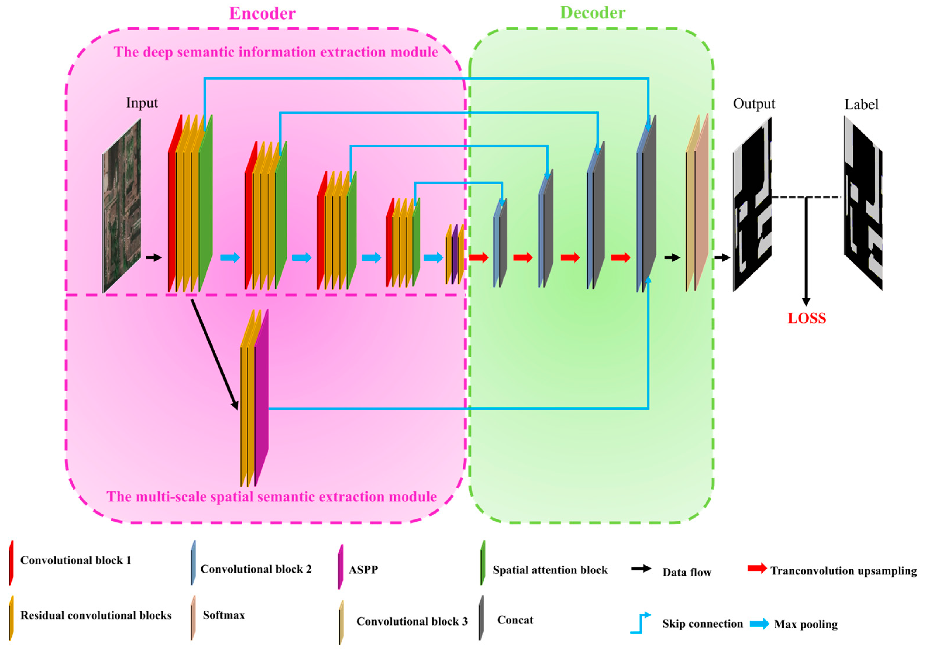
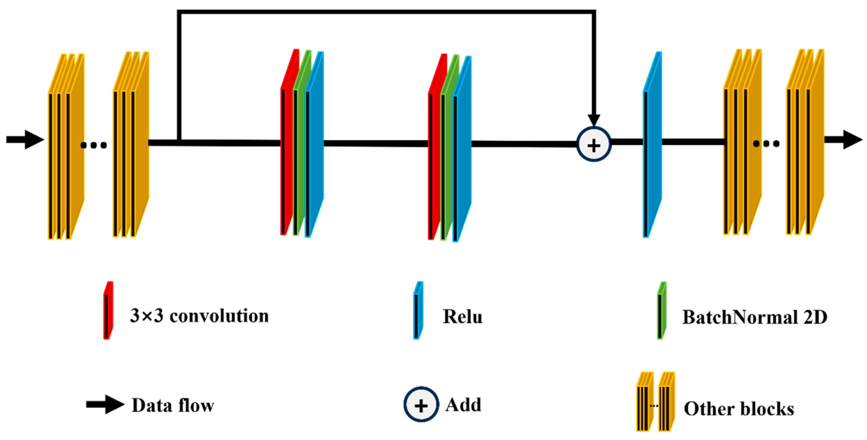
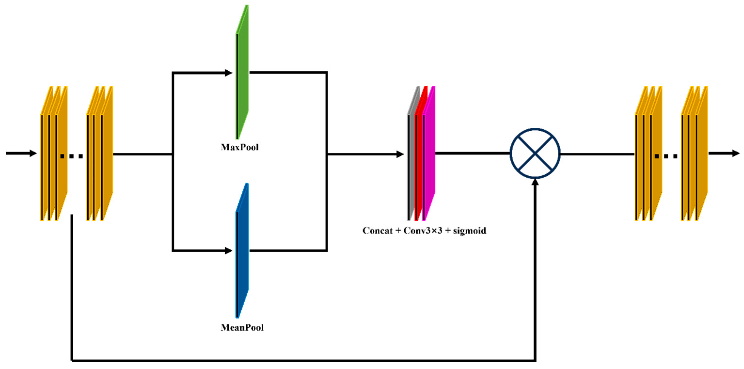
3.1. MFFNet
3.2. Evaluation Metrics
4. Results
4.1. Experimental Environment and Configuration
4.2. Experimental Results
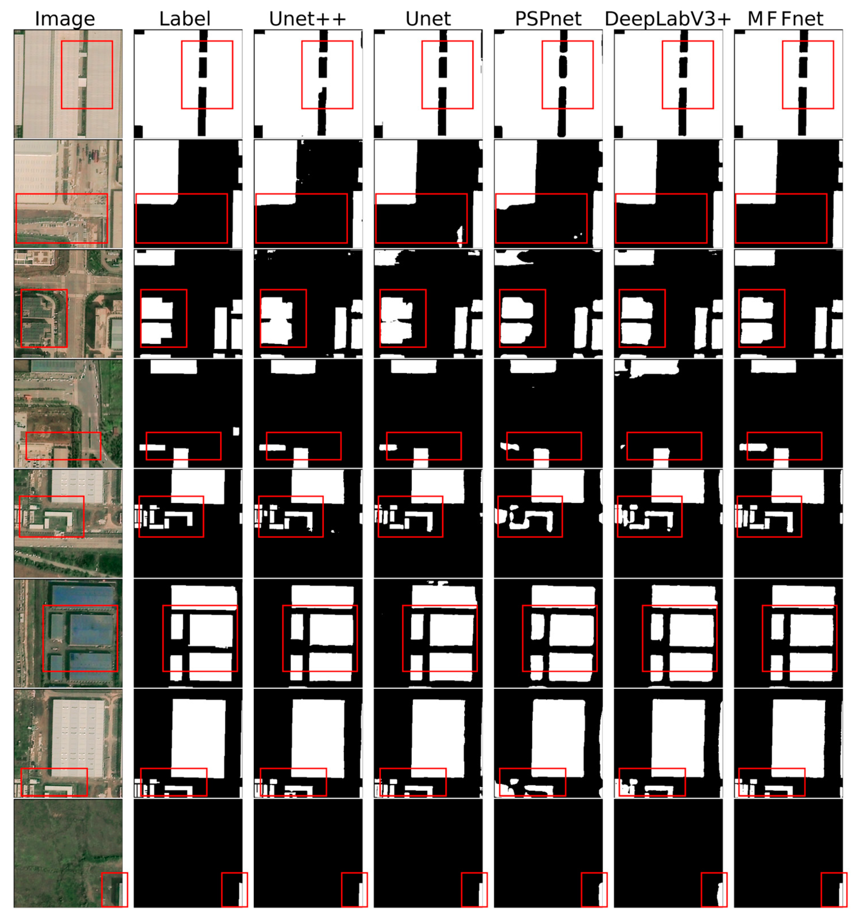
4.2.1. Jilin-1 Dataset
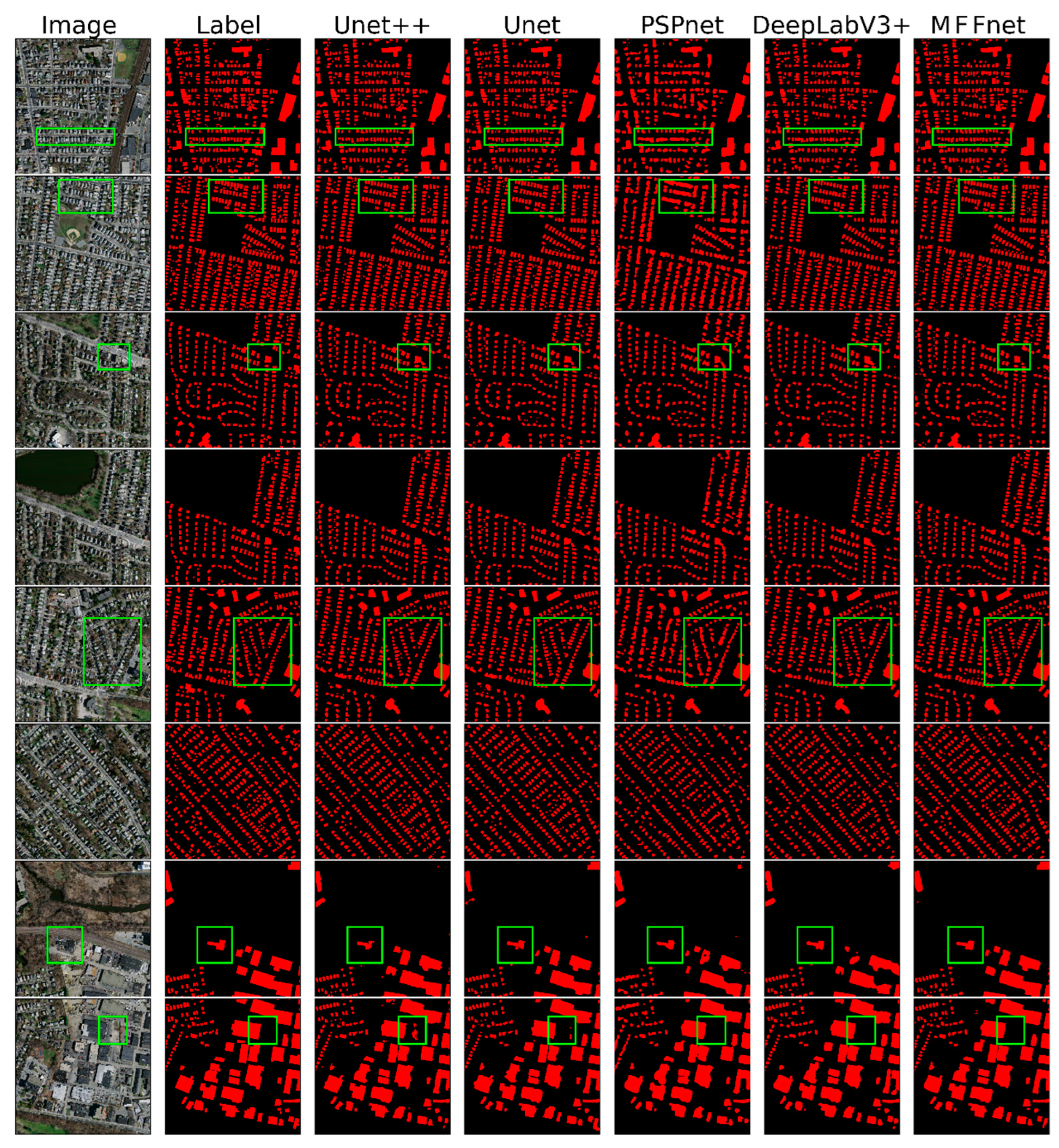
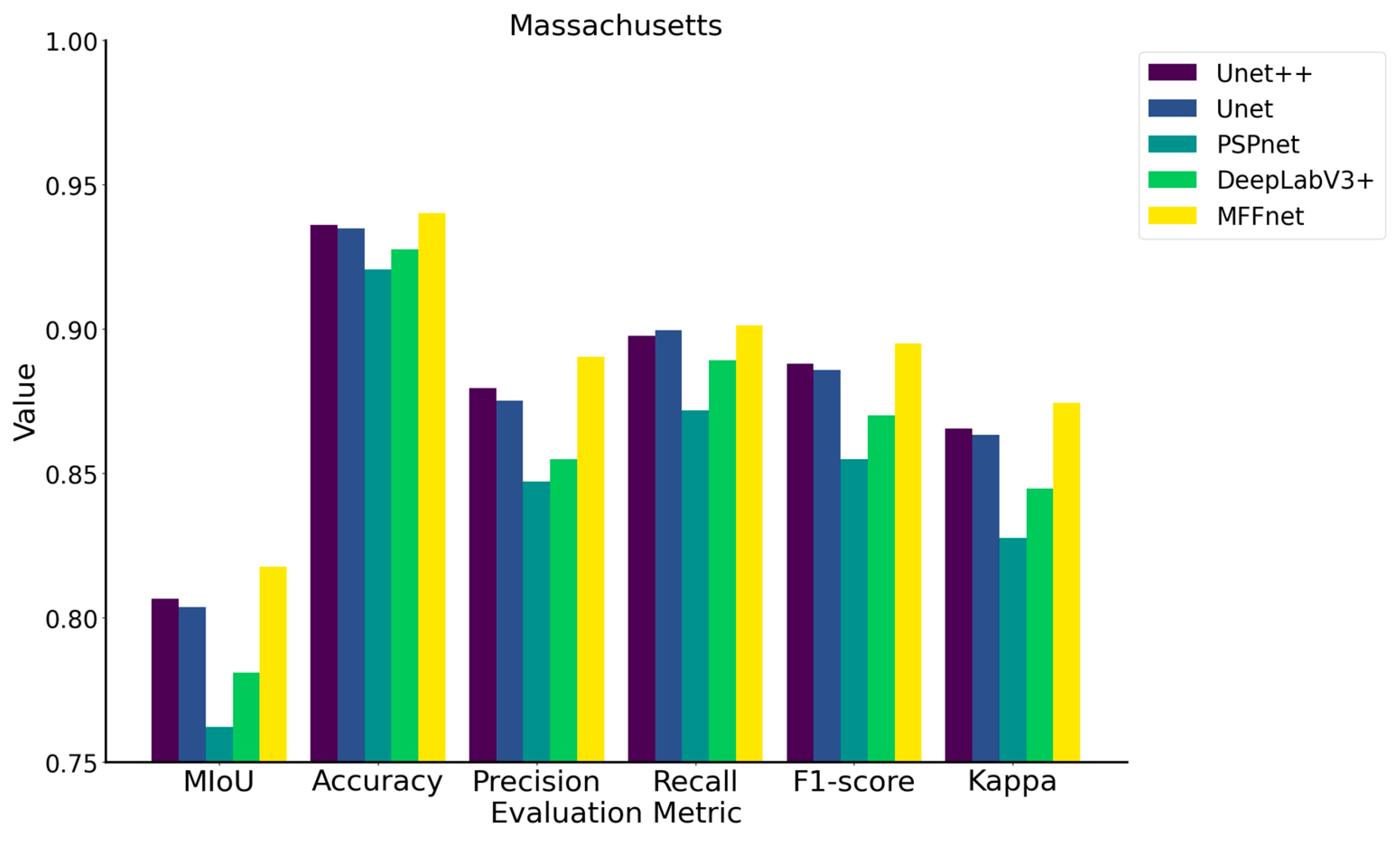
4.2.2. Massachusetts Building Dataset
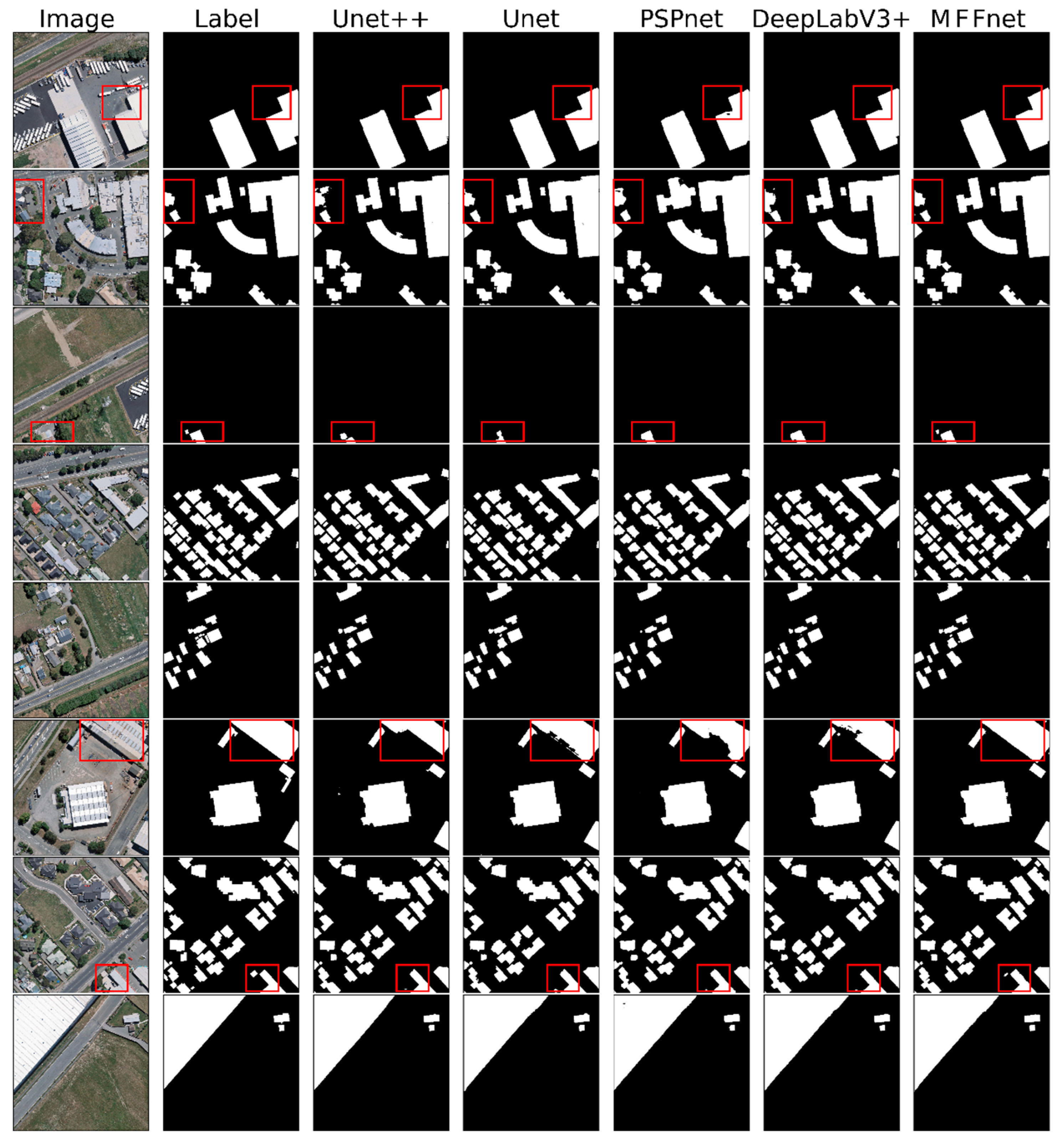
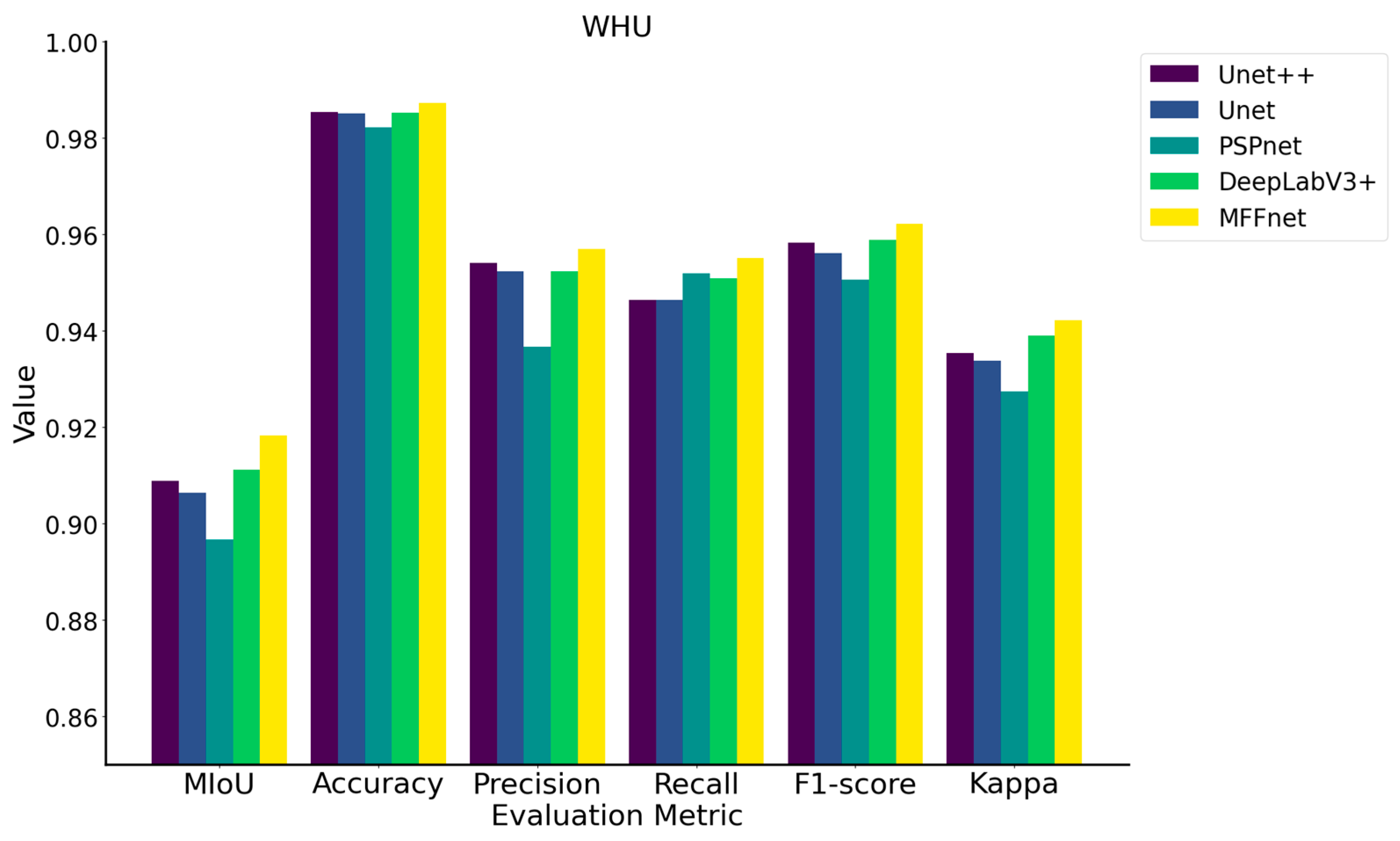
4.2.3. WHU Building Dataset
5. Discussion
6. Conclusions
Author Contributions
Funding
Institutional Review Board Statement
Informed Consent Statement
Data Availability Statement
Acknowledgments
Conflicts of Interest
References
- Shao, Z.; Cheng, T.; Fu, H.; Li, D.; Huang, X. Emerging Issues in Mapping Urban Impervious Surfaces Using High-Resolution Remote Sensing Images. Remote Sens. 2023, 15, 2562. [Google Scholar] [CrossRef]
- Cheng, D.; Meng, G.; Cheng, G.; Pan, C. SeNet: Structured Edge Network for Sea–Land Segmentation. IEEE Geosci. Remote Sens. Lett. 2017, 14, 247–251. [Google Scholar] [CrossRef]
- Zhang, B.; Wang, C.; Shen, Y.; Liu, Y. Fully Connected Conditional Random Fields for High-Resolution Remote Sensing Land Use/Land Cover Classification with Convolutional Neural Networks. Remote Sens. 2018, 10, 1889. [Google Scholar] [CrossRef]
- Park, N.W.; Chi, K.H. Quantitative assessment of landslide susceptibility using high-resolution remote sensing data and a generalized additive model. Int. J. Remote Sens. 2010, 29, 247–264. [Google Scholar] [CrossRef]
- Qiu, Y.; Wu, F.; Yin, J.; Liu, C.; Gong, X.; Wang, A. MSL-Net: An Efficient Network for Building Extraction from Aerial Imagery. Remote Sens. 2022, 14, 3914. [Google Scholar] [CrossRef]
- Wang, H.; Miao, F. Building extraction from remote sensing images using deep residual U-Net. Eur. J. Remote Sens. 2022, 55, 71–85. [Google Scholar] [CrossRef]
- Sirmaçek, B.; Ünsalan, C. Building Detection from Aerial Images using Invariant Color Features and Shadow Information. In Proceedings of the 23rd International Symposium on Computer and Information Sciences 2008, Istanbul, Turkey, 27–29 October 2008; pp. 6–10. [Google Scholar]
- Chen, R.; Li, X.; Li, J. Object-Based Features for House Detection from RGB High-Resolution Images. Remote Sens. 2018, 10, 451. [Google Scholar] [CrossRef]
- Du, S.H.; Zhang, F.L.; Zhang, X.Y. Semantic classification of urban buildings combining VHR image and GIS data: An improved random forest approach. ISPRS J. Photogramm. Remote Sens. 2015, 105, 107–119. [Google Scholar] [CrossRef]
- Tong, X.; Xie, H.; Weng, Q. Urban Land Cover Classification with Airborne Hyperspectral Data: What Features to Use? IEEE J. Sel. Top. Appl. Earth Obs. Remote Sens. 2014, 7, 3998–4009. [Google Scholar] [CrossRef]
- Huang, L.; Zhu, J.; Qiu, M.; Li, X.; Zhu, S. CA-BASNet: A Building Extraction Network in High Spatial Resolution Remote Sensing Images. Sustainability 2022, 14, 11633. [Google Scholar] [CrossRef]
- Wang, Y.; Zeng, X.; Liao, X.; Zhuang, D. B-FGC-Net: A Building Extraction Network from High Resolution Remote Sensing Imagery. Remote Sens. 2022, 14, 269. [Google Scholar] [CrossRef]
- Liu, J.; Wang, S.; Hou, X.; Song, W. A deep residual learning serial segmentation network for extracting buildings from remote sensing imagery. Int. J. Remote Sens. 2020, 41, 5573–5587. [Google Scholar] [CrossRef]
- Krizhevsky, A.; Sutskever, I.; Hinton, G.E. ImageNet Classification with Deep Convolutional Neural Networks. Commun. ACM 2017, 60, 84–90. [Google Scholar] [CrossRef]
- Simonyan, K.; Zisserman, A. Very deep convolutional networks for large-scale image recognition. arXiv 2014, arXiv:1409.1556. [Google Scholar]
- Szegedy, C.; Liu, W.; Jia, Y.Q.; Sermanet, P.; Reed, S.; Anguelov, D.; Erhan, D.; Vanhoucke, V.; Rabinovich, A. Going Deeper with Convolutions. In Proceedings of the CVPR IEEE, Boston, MA, USA, 7–12 June 2015; pp. 1–9. [Google Scholar] [CrossRef]
- He, K.M.; Zhang, X.Y.; Ren, S.Q.; Sun, J. Deep Residual Learning for Image Recognition. In Proceedings of the 2016 IEEE Conference on Computer Vision and Pattern Recognition (Cvpr) 2016, Las Vegas, NV, USA, 27–30 June 2016; pp. 770–778. [Google Scholar] [CrossRef]
- Long, J.; Shelhamer, E.; Darrell, T. Fully convolutional networks for semantic segmentation. In Proceedings of the IEEE Conference on Computer Vision and Pattern Recognition, Boston, MA, USA, 7–12 June 2015; pp. 3431–3440. [Google Scholar]
- Sun, W.; Wang, R. Fully Convolutional Networks for Semantic Segmentation of very High Resolution Remotely Sensed Images Combined with DSM. IEEE Geosci. Remote Sens. Lett. 2018, 15, 474–478. [Google Scholar] [CrossRef]
- Badrinarayanan, V.; Kendall, A.; Cipolla, R. SegNet: A Deep Convolutional Encoder-Decoder Architecture for Image Segmentation. IEEE Trans. Pattern Anal. 2017, 39, 2481–2495. [Google Scholar] [CrossRef]
- Ronneberger, O.; Fischer, P.; Brox, T. U-Net: Convolutional Networks for Biomedical Image Segmentation. Lect. Notes Comput. Sci. 2015, 9351, 234–241. [Google Scholar] [CrossRef]
- Chen, L.C.; Papandreou, G.; Kokkinos, I.; Murphy, K.; Yuille, A.L. DeepLab: Semantic Image Segmentation with Deep Convolutional Nets, Atrous Convolution, and Fully Connected CRFs. IEEE Trans. Pattern Anal. 2018, 40, 834–848. [Google Scholar] [CrossRef]
- Chen, L.C.E.; Zhu, Y.K.; Papandreou, G.; Schroff, F.; Adam, H. Encoder-Decoder with Atrous Separable Convolution for Semantic Image Segmentation. In Proceedings of the Computer Vision—ECCV, Munich, Germany, 8–14 September 2018; Part Vii. Volume 11211, pp. 833–851. [Google Scholar] [CrossRef]
- Zhao, H.S.; Shi, J.P.; Qi, X.J.; Wang, X.G.; Jia, J.Y. Pyramid Scene Parsing Network. In Proceedings of the 30th IEEE Conference on Computer Vision and Pattern Recognition (Cvpr 2017), Honolulu, HI, USA, 21–26 July 2017; pp. 6230–6239. [Google Scholar] [CrossRef]
- Li, X.; Li, Y.; Ai, J.; Shu, Z.; Xia, J.; Xia, Y. Semantic segmentation of UAV remote sensing images based on edge feature fusing and multi-level upsampling integrated with Deeplabv3. PLoS ONE 2023, 18, e0279097. [Google Scholar] [CrossRef]
- Wang, X.; Jing, S.; Dai, H.; Shi, A. High-resolution remote sensing images semantic segmentation using improved UNet and SegNet. Comput. Electr. Eng. 2023, 108, 108734. [Google Scholar] [CrossRef]
- Daudt, R.C.; Le Saux, B.; Boulch, A. Fully Convolutional Siamese Networks for Change Detection. In Proceedings of the 2018 25th IEEE International Conference on Image Processing (ICIP), Athens, Greece, 7–10 October 2018; pp. 4063–4067. [Google Scholar]
- Chen, Z.; Wang, C.; Li, J.; Fan, W.; Du, J.; Zhong, B. Adaboost-like End-to-End multiple lightweight U-nets for road extraction from optical remote sensing images. Int. J. Appl. Earth Obs. Geoinf. 2021, 100, 102341. [Google Scholar] [CrossRef]
- Hu, J.; Shen, L.; Sun, G. Squeeze-and-excitation networks. In Proceedings of the IEEE Conference on Computer Vision and Pattern Recognition, Salt Lake City, UT, USA, 18–23 June 2018; pp. 7132–7141. [Google Scholar]
- Chen, H.; He, Y.; Zhang, L.; Yao, S.; Yang, W.; Fang, Y.; Liu, Y.; Gao, B. A landslide extraction method of channel attention mechanism U-Net network based on Sentinel-2A remote sensing images. Int. J. Digit. Earth 2023, 16, 552–577. [Google Scholar] [CrossRef]
- Yu, Y.; Liu, C.; Gao, J.; Jin, S.; Jiang, X.; Jiang, M.; Zhang, H.; Zhang, Y. Building Extraction from Remote Sensing Imagery with a High-Resolution Capsule Network. IEEE Geosci. Remote Sens. Lett. 2022, 19, 8015905. [Google Scholar] [CrossRef]
- Eftekhari, A.; Samadzadegan, F.; Dadrass Javan, F. Building change detection using the parallel spatial-channel attention block and edge-guided deep network. Int. J. Appl. Earth Obs. Geoinf. 2023, 117, 103180. [Google Scholar] [CrossRef]
- Yuan, X.; Shi, J.; Gu, L. A review of deep learning methods for semantic segmentation of remote sensing imagery. Expert Syst. Appl. 2021, 169, 114417. [Google Scholar] [CrossRef]
- Zhou, Y.; Chen, Z.L.; Wang, B.; Li, S.J.; Liu, H.; Xu, D.Z.; Ma, C. BOMSC-Net: Boundary Optimization and Multi-Scale Context Awareness Based Building Extraction from High-Resolution Remote Sensing Imagery. IEEE Trans. Geosci. Remote Sens. 2022, 60, 5618617. [Google Scholar] [CrossRef]
- Alsabhan, W.; Alotaiby, T. Automatic Building Extraction on Satellite Images Using Unet and ResNet50. Comput. Intell. Neurosci. 2022, 2022, 5008854. [Google Scholar] [CrossRef]
- Ji, S.P.; Wei, S.Q.; Lu, M. Fully Convolutional Networks for Multisource Building Extraction from an Open Aerial and Satellite Imagery Data Set. IEEE Trans. Geosci. Remote Sens. 2019, 57, 574–586. [Google Scholar] [CrossRef]


| Model | MIoU | Accuracy | Precision | Recall | F1-Score | Kappa |
|---|---|---|---|---|---|---|
| UNet++ | 86.66% | 95.46% | 92.91% | 92.70% | 92.85% | 90.21% |
| UNet | 86.51% | 95.66% | 92.81% | 92.53% | 92.68% | 90.05% |
| PSPNet | 85.06% | 95.40% | 91.26% | 92.16% | 91.81% | 89.06% |
| DeepLabV3+ | 86.97% | 96.12% | 93.01% | 92.74% | 92.99% | 90.48% |
| MFFNet | 89.69% | 97.05% | 94.66% | 94.25% | 94.82% | 92.63% |
| Model | MIoU | Accuracy | Precision | Recall | F1-Score | Kappa |
|---|---|---|---|---|---|---|
| UNet++ | 80.64% | 93.60% | 87.94% | 89.76% | 88.79% | 86.54% |
| UNet | 80.36% | 93.48% | 87.50% | 89.94% | 88.58% | 86.32% |
| PSPNet | 76.19% | 92.05% | 84.70% | 87.18% | 85.48% | 82.74% |
| DeepLabV3+ | 78.08% | 92.74% | 85.49% | 88.92% | 86.99% | 84.47% |
| MFFNet | 81.76% | 94.00% | 89.02% | 90.11% | 89.50% | 87.43% |
| Model | MIoU | Accuracy | Precision | Recall | F1-Score | Kappa |
|---|---|---|---|---|---|---|
| UNet++ | 90.88% | 98.54% | 95.40% | 94.63% | 95.82% | 93.53% |
| UNet | 90.64% | 98.50% | 95.23% | 94.64% | 95.61% | 93.38% |
| PSPNet | 89.67% | 98.22% | 93.66% | 95.18% | 95.05% | 92.74% |
| DeepLabV3+ | 91.12% | 98.52% | 95.23% | 95.09% | 95.88% | 93.89% |
| MFFNet | 91.82% | 98.73% | 95.69% | 95.50% | 96.22% | 94.22% |
| Datasets | Model | MIoU | Accuracy | Precise | Recall | F1-Score | Kappa |
|---|---|---|---|---|---|---|---|
| Jilin-1 | MFFNet | 89.69% | 97.05% | 94.66% | 94.25% | 94.82% | 92.63% |
| MFFNet (without ASPP) | 88.70% | 96.66% | 94.14% | 93.63% | 94.22% | 91.90% | |
| ViT | 89.27% | 95.60% | 94.42% | 94.10 | 94.12% | 92.62% | |
| Massachusetts | MFFNet | 81.76% | 94.00% | 89.02% | 90.11% | 89.50% | 87.43% |
| MFFNet (without ASPP) | 81.07% | 93.69% | 88.61% | 89.61% | 89.04% | 86.86% | |
| ViT | 79.15% | 93.07% | 86.78% | 88.91% | 87.76% | 85.35% | |
| WHU | MFFNet | 91.82% | 98.73% | 95.69% | 95.50% | 96.22% | 94.22% |
| MFFNet (without ASPP) | 91.94% | 98.78% | 95.81% | 95.55% | 96.42% | 94.28% | |
| ViT | 92.10% | 98.50% | 95.71% | 95.83% | 95.72% | 95.18% |
Disclaimer/Publisher’s Note: The statements, opinions and data contained in all publications are solely those of the individual author(s) and contributor(s) and not of MDPI and/or the editor(s). MDPI and/or the editor(s) disclaim responsibility for any injury to people or property resulting from any ideas, methods, instructions or products referred to in the content. |
© 2023 by the authors. Licensee MDPI, Basel, Switzerland. This article is an open access article distributed under the terms and conditions of the Creative Commons Attribution (CC BY) license (https://creativecommons.org/licenses/by/4.0/).
Share and Cite
Liu, K.; Xi, Y.; Liu, J.; Zhou, W.; Zhang, Y. MFFNet: A Building Extraction Network for Multi-Source High-Resolution Remote Sensing Data. Appl. Sci. 2023, 13, 13067. https://doi.org/10.3390/app132413067
Liu K, Xi Y, Liu J, Zhou W, Zhang Y. MFFNet: A Building Extraction Network for Multi-Source High-Resolution Remote Sensing Data. Applied Sciences. 2023; 13(24):13067. https://doi.org/10.3390/app132413067
Chicago/Turabian StyleLiu, Keliang, Yantao Xi, Junrong Liu, Wangyan Zhou, and Yidan Zhang. 2023. "MFFNet: A Building Extraction Network for Multi-Source High-Resolution Remote Sensing Data" Applied Sciences 13, no. 24: 13067. https://doi.org/10.3390/app132413067
APA StyleLiu, K., Xi, Y., Liu, J., Zhou, W., & Zhang, Y. (2023). MFFNet: A Building Extraction Network for Multi-Source High-Resolution Remote Sensing Data. Applied Sciences, 13(24), 13067. https://doi.org/10.3390/app132413067