Intersatellite and Downlink Agile Attitude Maneuvers

Abstract

This research is focused on the problem of agile attitude maneuvering, aimed at the precise pointing of a satellite forming a typical constellation in low Earth orbit. We consider two different operational scenarios: (a) pointing toward a specific ground station, located on the Earth surface (for downlink data routing), and (b) pointing toward a companion satellite (for establishing an intersatellite connection). The two preceding operational requirements can both be formulated as attitude tracking problems. In this study, we use an inertia-free nonlinear attitude control algorithm based on rotation matrices and possessing remarkable stability properties, in conjunction with a pyramidal array of single-gimbal control momentum gyroscopes. Numerical simulations, in both nominal and nonnominal flight conditions, demonstrate that the attitude control architecture proposed in this work is effective for the purpose of performing agile attitude maneuvering, aimed at precise pointing during downlink and intersat data routing.

1. Introduction

The use of large satellite constellations, placed in low Earth orbits and tailored to enhancing global connectivity, has attracted strong interest since the 90s. Some programs (Teledesic, Skybridge, Celestri) were canceled before launch and only a few systems (e.g., Iridium and Globalstar) became operational in the 90s [1,2,3,4]. Comparetto [5] and Dumont [6] reviewed some of these constellation architectures, while Evans [7] focused on a wider class of configurations, also involving geosynchronous and medium-altitude orbits.

In recent years, a renewed interest is leading some private ventures to completing the deployment of large constellations, tailored to providing global broadband coverage for high-speed internet access, especially for rural and remote areas, all around the world. Most recently, the first satellites equipped with laser technology were launched. In a recent publication, del Portillo et al. [8] provide a comprehensive analysis of three large satellite constellations, already launched (or being delivered) by SpaceX, OneWeb, and Telesat, while identifying some major challenges related to similar systems. Collision avoidance represents one such challenge, investigated by Le May et al. [9], and imposes continuous monitoring and a high degree of automation. Efficient geographical data routing is another fundamental systemic aspect, and is investigated by Roth et al. [10].

Information sharing in large constellations implies the capability of performing agile attitude maneuvers, in the context of two different operational scenarios: (a) pointing toward a specific location on Earth, and (b) pointing toward a companion satellite. In both cases, the attitude control system of the satellite of interest must be able to track a time-varying pointing direction, to perform either (a) data acquisition or downlink connection, or (b) an intersatellite connection for data sharing. The two preceding operational requirements can be both formulated as attitude tracking problems.

The design, implementation, and testing of algorithms for slewing or tracking maneuvers is an active research area, with the final objective of identifying suitable feedback schemes, effective and accurate for autonomous attitude control. Recent contributions highlight the growing interest toward agile attitude maneuvers for remote sensing applications [11,12,13,14]. In particular, Poche et al. [13] investigate autonomous guidance for slewing maneuvers, while taking actuator limitations into account. Gordon et al. [15] consider the effects of model fidelity and parameter uncertainty on the performance of a feedback feedforward algorithm for attitude tracking of a satellite with flexible appendages. Marshall and Pellegrino [16] show that, contrary to common assumptions, the available angular momentum and torque, supplied by the actuation system, impose more restrictive limits on maneuverability than the dynamics of the spacecraft, modeled as a flexible system. Different representations for attitude kinematics are available. Unlike Euler angles, Euler parameters (quaternions) are suitable for large reorientation and attitude tracking maneuvers. Recently, Yefymenko and Kudermetov [17] proposed second-order quaternionic equations for attitude kinematics and dynamics. In the scientific literature, several contributions employed the Euler parameters as the kinematics variables [18,19,20]. The final goal was in identifying feedback control laws that enjoy quasi-global stability properties. Their main drawback is represented by the need of accurate knowledge regarding the spacecraft mass distribution, in particular its instantaneous inertia matrix. This information may be not sufficiently accurate, and this circumstance can compromise the pointing maneuver or reduce its precision. Recently, some inertia-free algorithms were proposed that do not require any accurate knowledge of the spacecraft mass distribution [21,22]. In particular, Sanyal et al. [21] designed an inertia-free attitude control algorithm that employs rotation matrices. The latter representation has the additional advantage of uniqueness when compared to Euler parameters.

This research is based on the conference paper [23], and addresses the problem of agile attitude maneuvering, aimed at precise pointing of a satellite that forms a typical constellation in low-altitude Earth orbit. More specifically, two different operational scenarios are considered: (a) pointing toward a specific ground station, located on the Earth surface, and (b) pointing toward a companion satellite. In both cases, the attitude control system of the satellite of interest must be able to track a time-varying pointing direction. To achieve this, the following study employs an inertia-free nonlinear attitude control algorithm based on rotation matrices [21] and possessing remarkable stability properties. Gain tuning for this scheme involves the instantaneous angular velocity components, as well as further quantities related to the maximum available torque and the expected transient time. Because the orbital dynamics relative to the target—either the ground station (a) or a companion satellite (b)—is relatively fast, agile attitude maneuvering is mandatory to complete the required data routing operations. With this intent, this study considers the use of a pyramidal array of single-gimbal control momentum gyroscopes with constant rotor speed. Their dynamical interaction with the spacecraft is accurately modeled, to identify the equivalent torque transferred to the satellite. The main challenge in using these devices is represented by the identification of an effective steering law, capable of avoiding singularities. Several approaches are available to address this issue, e.g., the use of null motion. In this study, singular direction avoidance based on singular value decomposition of the actuation matrix is used. However, the inclusion of the actuation dynamics implies that the commanded torque, yielded by the nonlinear control algorithm, differs from the actual torque transferred to the vehicle. This circumstance implies that the analytical asymptotic stability properties proven for the attitude control algorithm do not hold for the overall system that includes the actuator dynamics, strictly speaking. Hence, numerical evidence must support the use and effectiveness of nonlinear attitude control with actuation modeling. The satellite of interest is assumed to perform a maneuver composed of two phases: (i) attitude tracking aimed at continuous pointing toward the target and (ii) attitude reorientation, in preparation for tracking the next target. Effectiveness of the attitude control and actuation architecture proposed in this study is being investigated numerically, with reference to the two operational scenarios of interest, i.e., continuous pointing of either a ground station (a) or a companion satellite (b), during the respective time intervals of visibility. Numerical analysis is being performed in both nominal and nonnominal conditions, associated with stochastic displacements in the initial attitude and angular rate.

2. Spacecraft Attitude Dynamics

The spacecraft is modeled as a rigid body, and has an instantaneous orientation associated with vectrix $\underline{\underline{B}}$ [24],

$$\underline{\underline{B}}=\left[\begin{array}{ccc}{\widehat{b}}_1& {\widehat{b}}_2& {\widehat{b}}_3\end{array}\right]$$

(1)

where $({\widehat{b}}_1,{\widehat{b}}_2,{\widehat{b}}_3)$ are the unit vectors aligned with the body axes. In this study, the instantaneuos attitude is referred to $\underline{\underline{N}}$, which identifies the inertial reference frame, and is described through the direction cosine matrix. The attitude of the spacecraft is defined by $R=\underset{N\leftarrow B}{R}$, which is a rotation matrix such that ${\underline{\underline{N}}}^T=\underset{N\leftarrow B}{R}{\underline{\underline{B}}}^T$. The kinematics equation for R is

$$\dot{R}=R\tilde{\omega }$$

(2)

where $\tilde{\omega }$ is the skew-symmetric matrix associated with the components (along the body axes) of the angular velocity of the spacecraft relative to the inertial frame.

This research is focused on attitude tracking maneuvers, aimed at driving the actual spacecraft orientation toward the desired (commanded) attitude, while attaining the commanded angular rate. Meaningful variables in an attitude tracking problems are

$$\begin{array}{cc}\hfill & {\underline{\omega }}_e=\underline{\omega }-R_e^T{\underline{\omega }}_c^{\left(C\right)}\hfill \end{array}$$

(3)

$$\begin{array}{cc}\hfill & {\Phi }_e={cos}^{-1}\left({\displaystyle \frac{1}{2}}\left[\mathrm{trace}\left(R_e\right)-1\right]\right)\hfill \end{array}$$

(4)

In Equations (3) and (4) $R_e=\underset{C\leftarrow B}{R}$ is the error matrix, which is a rotation matrix such that ${\underline{\underline{C}}}^T=\underset{C\leftarrow B}{R}{\underline{\underline{B}}}^T$ while ${\underline{\omega }}_c^{\left(C\right)}$ and $\underline{\omega }$ are two $(3\times 1)$-vectors that contain, respectively, the components of the desired angular velocity (in $\underline{\underline{C}}$) and the actual angular velocity (in $\underline{\underline{B}}$).

The transient behavior of the system can be described using the mean (integral) values of ${\Phi }_e$ and $|{\underline{\omega }}_e|$. Let $n_p$ be the number of visible passes; $t_{0_i}$ and $t_{f_i}$ denote the times at which the i-th tracking phase begins and ends, respectively. The mean values of the variables defined in Equations (3) and (4) are

$$\begin{array}{cc}\hfill & {\overline{\Phi }}_{e_i}={\displaystyle \frac{1}{t_{f_i}-t_{0_i}}}{\int }_{t_{0_i}}^{t_{f_i}}{\Phi }_e\left(t\right)dti=1,\dots ,n_p\hfill \end{array}$$

(5)

$$\begin{array}{cc}\hfill & {\overline{\omega }}_{e_i}={\displaystyle \frac{1}{t_{f_i}-t_{0_i}}}{\int }_{t_{0_i}}^{t_{f_i}}\left|{\underline{\omega }}_e\left(t\right)\right|dti=1,\dots ,n_p\hfill \end{array}$$

(6)

Since the center of mass C does not move during the maneuver, the attitude dynamics equations are decoupled from the trajectory equations. Expressed in terms of error angular velocity, they are given by [21]

$$\begin{array}{c}\hfill J_C^{\left(B\right)}{\underline{\dot{\omega }}}_e={\left[J_C^{\left(B\right)}\left({\underline{\omega }}_e+R_e^T{\underline{\omega }}_c^{\left(C\right)}\right)\right]}^{\sim }\left({\underline{\omega }}_e+R_e^T{\underline{\omega }}_c^{\left(C\right)}\right)+J_C^{\left(B\right)}\left({\tilde{\omega }}_e{R}_e^T{\underline{\omega }}_c^{\left(C\right)}-R_e^T{\underline{\dot{\omega }}}_c^{\left(C\right)}\right)+{\underline{T}}_c+{\underline{M}}_C\end{array}$$

(7)

In Equation (7) ${\underline{M}}_C$ is the vector that contains the sum of all external torques referred to the center of mass of the spacecraft, vector ${\underline{T}}_c$ is the commanded torque, $J_C^{\left(B\right)}$ is the inertia matrix, resolved in the body-fixed reference frame, with respect to the center of mass. Vectors ${\underline{M}}_C$, ${\underline{T}}_c$, and ${\underline{\omega }}_e$ are resolved in $\underline{\underline{B}}$, unlike ${\underline{\omega }}_c^{\left(C\right)}$.

The present research considers the satellite Türksat1B as an illustrative example of medium-size satellite [25], and assumes the following inertia matrix (obtained from the inertia matrix of Türksat1B):

$$J_C^{\left(B\right)}=\left[\begin{array}{ccc}3815& -15& -21\\ -15& 775& -21\\ -21& -21& 4050\end{array}\right]\mathrm{kg}\mathrm{m}{}^2$$

(8)

3. Nonlinear Attitude Control

In this analysis, the commanded torque is identified by using the algorithm presented in [21,26], which does not require perfect knowledge of the inertia matrix. This approach is based on the Lyapunov method and employs the rotation matrix as the attitude representation. The desired attitude is associated with vectrix $\underline{\underline{C}}$. The attitude control algorithm aims at determining the control torque such that the actual attitude of the spacecraft, associated with $\underset{N\leftarrow B}{R}$, pursues the commanded orientation, identified by the rotation matrix $R_c:=\underset{N\leftarrow C}{R}$. In this study, a tracking maneuver is considered, and the commanded frame $\underline{\underline{C}}$ is pursued. The commanded torque is obtained by using the algorithm presented in [21,26], and is given by

$$\begin{array}{c}\hfill {\underline{T}}_c=-{\widehat{J}}_C^{\left(B\right)}\tilde{\omega }\underline{\omega }-{\widehat{J}}_C^{\left(B\right)}(K_1\dot{\underline{S}}+{\tilde{\omega }}_e\underline{\omega }-R_e^T{\underline{\dot{\omega }}}_c^{\left(C\right)})-k_p\underline{S}-K_v({\underline{\omega }}_e+K_1\underline{S})\end{array}$$

(9)

Equation (9) represents a feedback control law, which supplies the commanded torque in terms of the variables R and $\underline{\omega }$. In Equation (9) $k_p$ is a constant, positive quantity, $K_1$ is a constant, diagonal, positive-definite matrix, $K_v$ is a positive-definite matrix, ${\widehat{J}}_C^{\left(B\right)}$ is the estimate of $J_C^{\left(B\right)}$. Vector $\underline{S}$ is related to the displacement of the actual attitude matrix R from $R_c$,

$$\underline{S}=\sum _{i=1}^3{a}_i{\left(R_e^T{\underline{e}}_i\right)}^{\sim }{\underline{e}}_i$$

(10)

where $a_i$ ($i=1,2,3$) denote arbitrary positive constants, whereas ${\underline{e}}_i$ represents the $i\text{–}th$ column vector of the canonical basis. The time derivative $\dot{\underline{S}}$ is

$$\dot{\underline{S}}=\sum _{i=1}^3{a}_i{\left[{\left(R_e^T{\underline{e}}_i\right)}^{\sim }{\underline{\omega }}_e\right]}^{\sim }{\underline{e}}_i$$

(11)

Let L be an operator that takes a (3 × 1)-vector as the input and yields a (3 × 6)-matrix, whereas $\underline{\gamma }$ collects the momenta and products of inertia, i.e.,

$$\begin{array}{cc}\hfill & L\left(\underline{\omega }\right)=\left[\begin{array}{cccccc}{\omega }_1& 0& 0& 0& {\omega }_3& {\omega }_2\\ 0& {\omega }_2& 0& {\omega }_3& 0& {\omega }_1\\ 0& 0& {\omega }_3& {\omega }_2& {\omega }_1& 0\end{array}\right]\hfill \end{array}$$

(12)

$$\begin{array}{cc}\hfill & \underline{\gamma }={\left[\begin{array}{cccccc}{J}_{11}& J_{22}& J_{33}& J_{23}& J_{13}& J_{12}\end{array}\right]}^T\hfill \end{array}$$

(13)

The preceding two definitions lead to

$$J_C^{\left(B\right)}\underline{\omega }=L\left(\underline{\omega }\right)\underline{\gamma }$$

(14)

Let $\widehat{\underline{\gamma }}$ be the vector that contains the estimate of $\underline{\gamma }$ and Q a constant, diagonal, positive-definite matrix. The governing equation that describes the time evolution of $\widehat{\underline{\gamma }}$ is [21]

$$\dot{\widehat{\underline{\gamma }}}=Q^{-1}[L^T\left(\underline{\omega }\right)\tilde{\omega }+L^T(K_1\dot{\underline{S}}+{\tilde{\omega }}_e\underline{\omega }-R_e^T{\underline{\dot{\omega }}}_c^{\left(C\right)})]({\underline{\omega }}_e+K_1\underline{S})$$

(15)

Gain selection takes advantage of the following formulas [21,26]:

$$k_p={\displaystyle \frac{{\alpha }_0}{\mathrm{trace}\left(\tilde{A}\right)}}$$

(16)

$$K_v={\beta }_0\left[\begin{array}{ccc}{\displaystyle \frac{1}{1+|{\omega }_1|}}& 0& 0\\ 0& {\displaystyle \frac{1}{1+|{\omega }_2|}}& 0\\ 0& 0& {\displaystyle \frac{1}{1+|{\omega }_3|}}\end{array}\right]$$

(17)

where ${\omega }_1$, ${\omega }_2$, and ${\omega }_3$ are the three instantaneous angular velocity components, $\tilde{A}$ is a diagonal matrix with elements $a_i$, whereas ${\alpha }_0$ and ${\beta }_0$ are two constant parameters, tuned as explained in [21,27], through numerical analysis.

4. Actuation

This section is focused on describing the dynamics of the attitude actuators and defining their steering law. In this research, attitude control is performed through an array of 4 Single-Gimbal Control Momentum Gyroscopes (SGCMGs). A SGCMG is a momentum exchange device, which can be modeled as a rotor with an additional degree of freedom, as depicted in Figure 1, where index j refers to the j-th device. It is composed of a wheel that rotates about an axis which can change its orientation. In fact, the rotor is linked to a gimbal that is able to vary the orientation of the axis of the wheel through a rotation by angle ${\theta }_1^{\left(j\right)}$ about axis ${\widehat{g}}_j$. When a rotation ${\theta }_1^{\left(j\right)}$ occurs the angular momentum of the wheel varies in direction and the reaction torque represents the control torque exerted on the spacecraft.

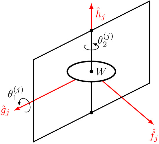
Figure 1. Schematic representation of Single-Gimbal Control Momentum Gyroscope.

M50 CMG, produced by Honeywell, is chosen as the actuator in this research. The characteristics of the device at hand are reported in Table 1, in terms of ${\omega }_R$ (velocity of the rotor), $I_S$ (axial moment of inertia), $I_T$ (transverse moment of inertia).

Table 1. M50 CMG Honeywell datasheet [28].

${\mathit{\omega }}_{\mathit{R}}$[rpm]	${\mathit{I}}_{\mathit{S}}$[kg m${}^2$]	${\mathit{I}}_{\mathit{T}}$[kg m${}^2$]
6500	0.1102	0.0551

Developing an effective steering law for SGCMGs represents a challenging task due to the existence of singular directions related to specific orientations of each device. The first step is in identifying the actual torque transferred to the spacecraft by an array of 4 SGCMGs.

4.1. Actuator Dynamics

Let ${\underline{\underline{W_0}}}^{\left(j\right)}$ denote the vectrix associated with the nominal orientation of the j-th wheel, which is the configuration for which ${\theta }_1^{\left(j\right)}$ = 0,

$${\underline{\underline{W_0}}}^{\left(j\right)}=\left[\begin{array}{ccc}{\widehat{w}}_1^{\left(j\right)}& {\widehat{w}}_2^{\left(j\right)}& {\widehat{w}}_3^{\left(j\right)}\end{array}\right]$$

(18)

Vectrix ${\underline{\underline{W_1}}}^{\left(j\right)}$ denotes the vectrix associated with the instantaneous orientation of the j-th wheel,

$${\underline{\underline{W_1}}}^{\left(j\right)}=\left[\begin{array}{ccc}{\widehat{g}}_j& {\widehat{f}}_j& {\widehat{h}}_j\end{array}\right]$$

(19)

Let $R_A^{\left(j\right)}$ represent the constant rotation matrix that describes the orientation of ${\underline{\underline{W_0}}}^{\left(j\right)}$ with respect to $\underline{\underline{B}}$ (i.e., the geometry of the mounting of the j-th gyroscope inside the spacecraft),

$${R_A^{\left(j\right)}}^T=\left[\begin{array}{ccc}{\underline{r}}_{A1}^{\left(j\right)}& {\underline{r}}_{A2}^{\left(j\right)}& {\underline{r}}_{A3}^{\left(j\right)}\end{array}\right]$$

(20)

$${{\underline{\underline{W_0}}}^{\left(j\right)}}^T=R_A^{\left(j\right)}{\underline{\underline{B}}}^T$$

(21)

The space vehicle is equipped with an array of four SGCMGs, which are mounted in a pyramidal arrangement (cf. Figure 2), where the angle $\beta$ between the faces and the base is assumed to equal 54.74°. This configuration is widely used in space missions thanks to the fact that it is associated with a nearly spherical momentum envelope [29]. The standard methodology of Eulerian dynamics [24,30] leads to describing the rotational dynamics of a system composed of a spacecraft with 4 SGCMGs, all characterized by constant rotor speed, denoted with ${\omega }_R^{\left(j\right)}$. The dynamics equation is

$$\begin{gathered} \begin{array}{cc}\hfill & J_C^{\left(B\right)}\underline{\dot{\omega }}={\underline{M}}_C-\tilde{\omega }{J}_C^{\left(B\right)}\underline{\omega }-{\dot{J}}_C^{\left(B\right)}\underline{\omega }+\tilde{\omega }\sum _{j=1}^4{I}_S^{\left(j\right)}{\omega }_R^{\left(j\right)}\left[sin\left({\theta }_1^{\left(j\right)}\right){\underline{r}}_{A2}^{\left(j\right)}-cos\left({\theta }_1^{\left(j\right)}\right){\underline{r}}_{A3}^{\left(j\right)}\right]+\hfill \end{array} \\ \begin{array}{c}\hfill +\sum _{j=1}^4\left\{I_S^{\left(j\right)}{\omega }_R^{\left(j\right)}\left[cos\left({\theta }_1^{\left(j\right)}\right){\underline{r}}_{A2}^{\left(j\right)}+sin\left({\theta }_1^{\left(j\right)}\right){\underline{r}}_{A3}^{\left(j\right)}\right]-\tilde{\omega }{I}_T^{\left(j\right)}{\underline{r}}_{A1}^{\left(j\right)}\right\}{\dot{\theta }}_1^{\left(j\right)}-\sum _{j=1}^4{I}_T^{\left(j\right)}{\underline{r}}_{A1}^{\left(j\right)}{\ddot{\theta }}_1^{\left(j\right)}\end{array} \end{gathered}$$

(22)

In Equation (22), $I_T^{\left(j\right)}$ and $I_S^{\left(j\right)}$ are the transverse and axial momenta of inertia of wheel j. The three terms with summation and the term related to the time derivative of the inertia matrix represent the actual control torque ${\underline{T}}_a$ applied to the system, due to the presence of the array of SGCMGs. In fact, from Equation (22), it is straightforward to recognize that if these terms vanish, the preceding equation reduces to the Euler’s equation of a single rigid body. The following quantities are introduced:

$$\begin{array}{cc}\hfill & \underline{\dot{\theta }}={\left[{\dot{\theta }}_1^{\left(1\right)}\cdots \cdots {\dot{\theta }}_1^{\left(4\right)}\right]}^T\hfill \end{array}$$

(23)

$$\begin{array}{cc}\hfill & \underline{\ddot{\theta }}={\left[{\ddot{\theta }}_1^{\left(1\right)}\cdots \cdots {\ddot{\theta }}_1^{\left(4\right)}\right]}^T\hfill \end{array}$$

(24)

$$\begin{array}{cc}\hfill & A=\left[I_S^{\left(1\right)}{\omega }_R^{\left(1\right)}{\underline{f}}_1\cdots \cdots I_S^{\left(4\right)}{\omega }_R^{\left(4\right)}{\underline{f}}_4\right]\hfill \end{array}$$

(25)

$$\begin{array}{cc}\hfill & B=\left[I_T^{\left(1\right)}{\underline{r}}_{A1}^{\left(1\right)}\cdots \cdots I_T^{\left(4\right)}{\underline{r}}_{A1}^{\left(4\right)}\right]\hfill \end{array}$$

(26)

where ${\underline{f}}_j$ is a ($3\times 1$)-vector that includes the components of ${\widehat{f}}_j$ in $\underline{\underline{B}}$. The actual torque is written in a compact way as

$$\begin{array}{cc}\hfill & {\underline{T}}_a=A\underline{\dot{\theta }}-B\underline{\ddot{\theta }}-{\dot{J}}_C^{\left(B\right)}\underline{\omega }-\tilde{\omega }B\underline{\dot{\theta }}+\tilde{\omega }\sum _{j=1}^4{I}_S^{\left(j\right)}{\omega }_R^{\left(j\right)}\left[sin\left({\theta }_1^{\left(j\right)}\right){\underline{r}}_{A2}^{\left(j\right)}-cos\left({\theta }_1^{\left(j\right)}\right){\underline{r}}_{A3}^{\left(j\right)}\right]\hfill \end{array}$$

(27)

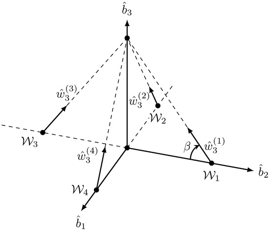
Figure 2. Pyramid array of SGCMGs used in the simulations.

4.2. Singular-Direction-Avoidance Steering Law

Equation (27) is simplified, for the purpose of deriving an effective, real-time steering law, by adopting the following assumptions:

• the term ${\dot{J}}_C^{\left(B\right)}$ is negligible, i.e., the overall inertia matrix is subject to modest time variations, due to the wheels rotation about their gimbal axes;
• the terms related to the second derivative of ${\theta }_1^{\left(j\right)}$ are negligible;
• $\left|{\omega }_R^{\left(j\right)}\right|\gg \left|\underline{\omega }\right|$, namely the rotor speeds are sufficiently high.

In this way, the only terms responsible for generating ${\underline{T}}_a$ are those not including the gyroscopic terms (i.e., terms with $\underline{\omega }$ or $\tilde{\omega }$). Under the preceding assumptions, the approximate actual torque ${\underline{T}}_a^{\left(A\right)}$ is along axis ${\widehat{f}}_j$ of each wheel and must equal ${\underline{T}}_c$, the commanded torque supplied by Equation (9),

$${\underline{T}}_a^{\left(A\right)}=A\underline{\dot{\theta }}={\underline{T}}_c$$

(28)

The Moore-Penrose pseudoinverse provides a solution for $\underline{\dot{\theta }}$ that minimizes $|\underline{\dot{\theta }}|$ ,

$$\underline{\dot{\theta }}=A^T{\left(A{A}^T\right)}^{-1}{\underline{T}}_c$$

(29)

However Equation (29) requires the inversion of matrix $A{A}^T$, which could be singular in some cases. In order to overcome this issue, this steering law is modified using a singularity avoidance strategy based on the singular value decomposition (SVD) [29,31]. To prevent $A{A}^T$ from becoming singular, one can replace it with

$$A^{\#}=(A{A}^T+X)$$

(30)

where matrix X is properly chosen in order to keep the system far from the singularity. Matrix A can be factorized trough SVD,

$$A=U\Sigma V^T$$

(31)

where the columns of matrices U and V contain, respectively, the left-singular and the right-singular vectors of A, whereas $\Sigma$ is the rectangular diagonal matrix containing the singular values. This algorithm introduces an error component in the actuated torque, which allows avoding the singularity. In particular, in this research SDA (Singularity Direction Avoidance) is used, based on introducing an error only along the direction associated with the minimum singular value of A. Matrix X is set to

$$X=U\left[\begin{array}{ccc}0& 0& 0\\ 0& 0& 0\\ 0& 0& \alpha \end{array}\right]U^T$$

(32)

where $\alpha$ is given by

$$\alpha ={\alpha }_{ref}{e}^{\left[-{\mu }_0\sqrt{detA{A}^T}\right]},{\alpha }_{ref},{\mu }_0\in {\mathbb{R}}^{+}$$

(33)

Symbols ${\alpha }_{ref}$ and ${\mu }_0$ denote two positive scalar quantities; $\alpha$ becomes relevant when the system is near the singularity, i.e., $det\left(A{A}^T\right)$≈ 0, whereas it is negligible when the system is far from singularity, i.e., $det\left(A{A}^T\right)$≫ 0. Taking advantage of SVD, the computation of $\underline{\dot{\theta }}$ does not require any inversion of $A^{\#}$. Denoting with ${\sigma }_1$, ${\sigma }_2$, ${\sigma }_3$ the singular values of A in decreasing order of magnitude, the gimbal angular rates $\underline{\dot{\theta }}$ (i.e., the steering law) is finally provided by

$$\underline{\dot{\theta }}=V\left[\begin{array}{ccc}{\displaystyle \frac{1}{{\sigma }_1}}& 0& 0\\ 0& {\displaystyle \frac{1}{{\sigma }_2}}& 0\\ 0& 0& {\displaystyle \frac{{\sigma }_3}{{\sigma }_3^2+\alpha }}\\ 0& 0& 0\end{array}\right]U^T{\underline{T}}_c$$

(34)

4.3. Net Motor Torque

The steering law obtained in the preceding subsection must be used in each arc that composes the overall attitude maneuver (i.e., tracking and slewing arcs, cf. Section 5 and Section 6). The commanded torque ${\underline{T}}_c$ is discontinuous across adjacent arcs, and this implies that $\underline{\dot{\theta }}$ is discontinuous as well. To improve the accuracy in modeling the dynamical system at hand, the steering law (34) is used to yield the commanded value of $\underline{\dot{\theta }}$, denoted with ${\underline{\dot{\theta }}}_c$. The real value of $\underline{\dot{\theta }}$ is found by integrating

$$\underline{\ddot{\theta }}={\displaystyle \frac{{\underline{\dot{\theta }}}_c-\underline{\dot{\theta }}}{{\tau }_{act}}}$$

(35)

where ${\tau }_{act}$ (set to 0.05 s) represents the time constant related to the reaction delay of the SGCMGs, while ${\underline{\dot{\theta }}}_c$ is obtained from Equation (34), with ${\underline{\dot{\theta }}}_c$ in place of $\underline{\dot{\theta }}$. Equation (35) is also useful for evaluating the angular accelerations of the gimbal axes, which allows determining the net motor torque $g_1^{\left(j\right)}$ applied to device j [30], i.e.,

$$\begin{array}{cc}\hfill & g_1^{\left(j\right)}=I_T^{\left(j\right)}{\ddot{\theta }}_1^{\left(j\right)}+I_T^{\left(j\right)}{\dot{\Omega }}_1^{\left(j\right)}+(I_S^{\left(j\right)}-I_T^{\left(j\right)}){\tilde{\Omega }}_2^{\left(j\right)}{\tilde{\Omega }}_3^{\left(j\right)}+I_S^{\left(j\right)}{\tilde{\Omega }}_2^{\left(j\right)}{\dot{\theta }}_2^{\left(j\right)}\hfill \end{array}$$

(36)

where $\underline{\Omega }$ and $\underline{\tilde{\Omega }}$ are ($3\times 1$)-vectors that include the components of the spacecraft angular velocity in $\underline{\underline{W_0}}$ and $\underline{\underline{W_1}}$, respectively.

5. Attitude Maneuvering for Downlink Connection

This section considers the problem of attitude tracking of a specified location on the Earth surface, for the purpose of establishing a downlink connection. This task must be performed only when the spacecraft is visible from the ground station. Thus, attititude maneuvering is split in two phases:

• attitude tracking, to point the spacecraft toward the ground station during visible passes, and
• attitude reorientation, aimed at gaining the correct pointing direction while waiting for the succeeding visible pass over the ground station.

Visibility of the ground station corresponds to an elevation angle $\epsilon$ greater than a minimum value ${\epsilon }_{min}$, related to the type of sensors mounted onboard the spacecraft. During attitude tracking, a time-varying attitude and angular velocity are pursued. In contrast, attitude reorientation represents a slewing maneuver, with zero angular rate and specified attitude, identified by the constant matrix $R_c$. This corresponds to aligning a specified body axis of the spacecraft with the direction where the ground station appears, as soon as it becomes visible. It is straightforward to recognize that the commanded attitude and the angular rate are discontinuous across the two trajectory arcs. As a result, the commanded torque is discontinuous at the same point (Equation (9)), as well as ${\underline{\dot{\theta }}}_c$ (Equation (34), with ${\underline{\dot{\theta }}}_c$ in place of $\underline{\dot{\theta }}$).

5.1. Commanded Attitude

The spacecraft attitude is referred to the Earth-centered inertial frame (ECI), associated with the following vectrix:

$$\underline{\underline{N}}=\left[\begin{array}{ccc}{\widehat{c}}_1& {\widehat{c}}_2& {\widehat{c}}_3\end{array}\right]$$

(37)

The final objective is in defining the commanded attitude, identified by $\underline{\underline{C}}$, in both phases, i.e., tracking and reorientation. In order to achieve correct pointing, a specified spacecraft body axis (i.e., ${\widehat{k}}_c$) must be aligned with the relative position vector that points from the spacecraft center of mass to the ground station.

As a first step, in the ECI-frame the ground station location is identified using spherical coordinates,

$${\overrightarrow{r}}_T=\left[\begin{array}{ccc}{\widehat{c}}_1& {\widehat{c}}_2& {\widehat{c}}_3\end{array}\right]\left[\begin{array}{c}{r}_{\oplus }cos\varphi cos\xi \\ r_{\oplus }cos\varphi sin\xi \\ r_{\oplus }sin\varphi \end{array}\right]$$

(38)

where $r_{\oplus }$ is the Earth radius, whereas $\xi$ is the absolute longitude and $\varphi$ is the latitude of the ground station. The absolute longitude $\xi$ is defined by the sum of the geographical longitude ${\lambda }_G$ and the Greenwich sidereal time ${\theta }_G$,

$$\xi ={\lambda }_G+{\theta }_G$$

(39)

where

$${\theta }_G={\theta }_{G_0}+{\omega }_{\oplus }(t-t_0)$$

(40)

In Equation (40), ${\theta }_{G_0}$ is the Greenwich sidereal time at epoch $t_0$, while ${\omega }_{\oplus }$ is the Earth rotation rate.

In the ECI-frame, the spacecraft position vector ${\overrightarrow{r}}_S$ can be written in terms of orbit elements,

$${\overrightarrow{r}}_S=\left[\begin{array}{ccc}r& 0& 0\end{array}\right]R_3\left({\theta }_t\right)R_1\left(i\right)R_3\left(\Omega \right)\left[\begin{array}{c}{\widehat{c}}_1\\ {\widehat{c}}_2\\ {\widehat{c}}_3\end{array}\right]$$

(41)

where $R_j\left(\chi \right)$ denotes the elementary rotation about axis j by angle $\chi$; angles ${\theta }_t$, i, and $\Omega$ are the instantaneous argument of altitude, inclination, and right ascension of the ascending node (RAAN); r is the instantaneous orbit radius. The argument of latitude equals

$${\theta }_t=\omega +{\theta }_{*}$$

(42)

where $\omega$ and ${\theta }_{*}$ represent, respectively, the argument of perigee and the true anomaly.

The commanded attitude is defined through the following relations:

$$\begin{array}{cc}\hfill & {\widehat{k}}_c={\displaystyle \frac{{\overrightarrow{r}}_T-{\overrightarrow{r}}_S}{\left|\right|{\overrightarrow{r}}_T-{\overrightarrow{r}}_S\left|\right|}}\hfill \end{array}$$

(43)

$$\begin{array}{cc}\hfill & {\widehat{l}}_c={\displaystyle \frac{{\widehat{k}}_c\times {\widehat{c}}_3}{\left|\right|{\widehat{k}}_c\times {\widehat{c}}_3\left|\right|}}\hfill \end{array}$$

(44)

$$\begin{array}{cc}\hfill & {\widehat{j}}_c={\widehat{k}}_c\times {\widehat{l}}_c\hfill \end{array}$$

(45)

The commanded attitude reference frame is illustrated in Figure 3. Using Equations (43)–(45), the unit vectors of the commanded attitude are resolved in the ECI-frame, and the rotation matrix that relates the commanded reference frame $\underline{\underline{C}}$ to the inertial reference frame $\underline{\underline{N}}$, denoted with $\underset{C\leftarrow N}{R}$, can be found in closed form. The next step is to obtain the analytical expression of the commanded angular velocity and its time derivative, starting from the kinematics equation for $\underset{C\leftarrow N}{R}$,

$$\dot{\underset{C\leftarrow N}{R}}=-{\tilde{\omega }}_c\underset{C\leftarrow N}{R}$$

(46)

leading to

$${\tilde{\omega }}_c=-\dot{\underset{C\leftarrow N}{R}}\underset{N\leftarrow C}{R}\to {\underline{\omega }}_c^{\left(C\right)}$$

(47)

Equation (47) allows finding the closed-form expression of the three components of ${\underline{\omega }}_c^{\left(C\right)}$, once $\underset{C\leftarrow N}{R}$ and $\dot{\underset{C\leftarrow N}{R}}$ are known. The latter can be written as the sum of three contributions:

$$\dot{\underset{C\leftarrow N}{R}}={\displaystyle \frac{\partial \underset{C\leftarrow N}{R}}{\partial \xi }}\dot{\xi }+{\displaystyle \frac{\partial \underset{C\leftarrow N}{R}}{\partial {\theta }_t}}\dot{{\theta }_t}+{\displaystyle \frac{\partial \underset{C\leftarrow N}{R}}{\partial {\theta }_{*}}}\dot{{\theta }_{*}}$$

(48)

where

$$\dot{\xi }={\dot{\theta }}_G={\omega }_{\oplus }$$

(49)

whereas the time derivative of the argument of latitude is [32]

$${\dot{\theta }}_t={\dot{\theta }}_{*}=\sqrt{{\displaystyle \frac{\mu }{p^3}}}{\left(1+ecos{\theta }_{*}\right)}^2$$

(50)

In Equation (50), $\mu$ is the gravitational parameter of the Earth, while p is the semilatus rectum of the operational orbit. The preceding equation assumes Keplerian motion, i.e., negligibility of orbit perturbations, which is a reasonable and rather accurate approximation over the timescale of a single repetition period. As previously remarked, Equation (47) leads to obtaining the three components of ${\underline{\omega }}_c^{\left(C\right)}$ in closed form. Their expressions are rather long and are not reported for the sake of conciseness.

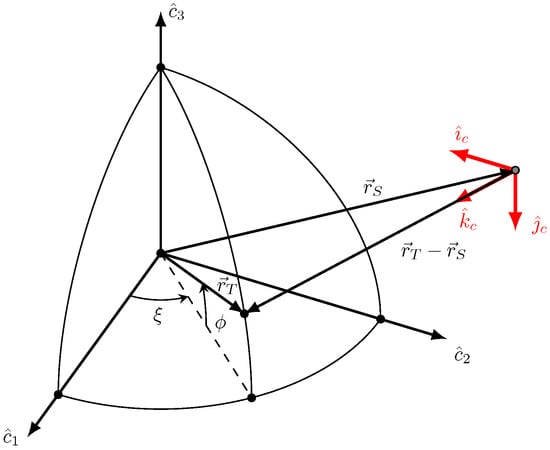
Figure 3. Geometry of the commanded attitude (downlink).

The last step consists of computing the time derivative of the commanded angular velocity,

$${\underline{\dot{\omega }}}_c^{\left(C\right)}={\displaystyle \frac{\partial {\underline{\omega }}_c^{\left(C\right)}}{\partial \xi }}\dot{\xi }+{\displaystyle \frac{\partial {\underline{\omega }}_c^{\left(C\right)}}{\partial {\theta }_t}}{\dot{\theta }}_t+{\displaystyle \frac{\partial {\underline{\omega }}_c^{\left(C\right)}}{\partial {\theta }_{*}}}{\dot{\theta }}_{*}$$

(51)

It is worth noting that the preceding developments lead to finding the desired attitude and angular rate in tracking intervals. The desired attitude in reorientation arcs can be found by predicting the inertial position of the ground station at the time when it becomes visible. Because this is a slewing maneuver, the corresponding commanded angular velocity ${\underline{\omega }}_c^{\left(C\right)}$ equals $\underline{0}$, as well as its time derivative.

5.2. Numerical Simulations in Nominal Conditions

In this work, the operational orbit is nearly circular, repeating, and with critical inclination. The repetition period equals 1 nodal day, and includes 15 nodal orbital periods. All orbit elements are reported in Table 2. The minimum elevation angle ${\epsilon }_{min}$ is set to 10°. Figure 4 depicts the elevation time history during the 5 visible passes (in a single repetition period) over the ground station, sited at geographical longitude of 9.4°and latitude of 39.7°. The initial attitude conditions are

$$\begin{array}{cc}\hfill & \underline{\omega }\left(t_0\right)={\left[\begin{array}{ccc}0& 0& 0\end{array}\right]}^T\hfill \end{array}$$

(52)

$$\begin{array}{cc}\hfill & \underline{\theta }\left(t_0\right)={\left[\begin{array}{cccc}0& {\displaystyle \frac{\pi }{4}}& {\displaystyle \frac{\pi }{2}}& {\displaystyle \frac{3\pi }{4}}\end{array}\right]}^T\hfill \end{array}$$

(53)

$$\begin{array}{cc}\hfill & \underline{\dot{\theta }}\left(t_0\right)={\left[\begin{array}{cccc}0& 0& 0& 0\end{array}\right]}^T\hfill \end{array}$$

(54)

$$\begin{array}{cc}\hfill & R\left(t_0\right)=I_{3\times 3}\hfill \end{array}$$

(55)

Table 2. Orbit elements of the operational orbit (semimajor axis a in [km], angles i, $\Omega$, $\omega$, and ${\theta }_{*}$ in [°]).

a	e	i	$\mathbf{\Omega }$	$\mathit{\omega }$	${\mathit{\theta }}_{*}\left({\mathit{t}}_0\right)$
6940.47	0.02	63.4	0	−90.0	0

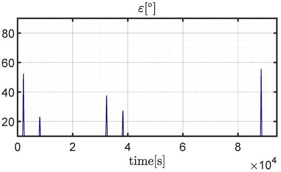
Figure 4. Elevation $\epsilon$(t)[°] during a repetition period.

Matrix Q, which is related to the inertia estimator dynamics (15), includes large values if the knowledge of the mass distribution of the spacecraft is satisfactory. Conversely, small values correspond to poor knowledge of it. For this simulation, Q is set to

$$Q={10}^{-8}{I}_{6\times 6}$$

(56)

The gains used in the numerical simulations are reported in Appendix A.

Figure 5 illustrates the eigenangle time history, which provides a clear indication of misalignment. This time history exhibits some spikes immediately after the end of tracking intervals, when the spacecraft must reorient to point toward the direction where the ground station will appear in the subsequent visible pass. Instead, during visible passes, the eigenangle reaches modest values, e.g., below 0.1°, as shown in Figure 6, referred to the fourth tracking interval. Figure 7 portrays the time histories of the components of the error angular velocity, which reach again their maximum values at the beginning of reorientation arcs. In contrast, during visible passes, these components quickly drop to zero, as illustrated in Figure 8. Precision in pointing is testified by the two mean values ${\overline{\Phi }}_{e_i}$ and ${\overline{\omega }}_{e_i}$, defined in Equations (5) and (6),

$$\begin{array}{cc}\hfill & {\overline{\Phi }}_{e_i}=6.20·{10}^{-2}°\hfill \end{array}$$

(57)

$$\begin{array}{cc}\hfill & {\overline{\omega }}_{e_i}=2.60·{10}^{-4} °/\mathrm{s}\hfill \end{array}$$

(58)

The actual torque components, depicted in Figure 9 and Figure 10, reach values of order of tens of Nm. The angular rates of the gimbals are portrayed in Figure 11 and Figure 12 and do not exceed 30 °/s. Finally, the time histories of net motor torques, shown in Figure 13, turn out to be of order of 1 Nm.

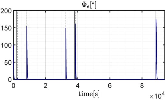
Figure 5. Pointing error ${\Phi }_e$(t)[°] during a repetition period.

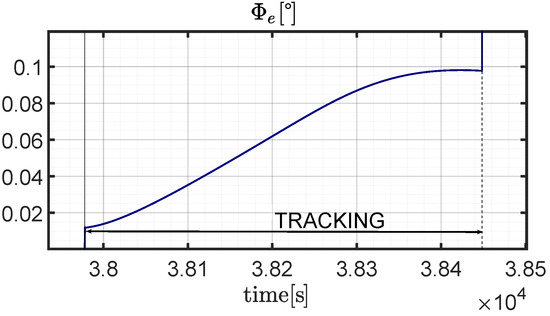
Figure 6. Pointing error ${\Phi }_e$(t)[°] during the fourth tracking interval.

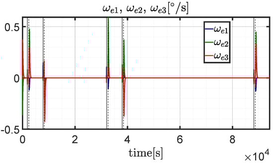
Figure 7. Components of the error angular velocity ${\omega }_{e1}$(t), ${\omega }_{e2}$(t), ${\omega }_{e3}$(t)[°/s] during a repetition period.

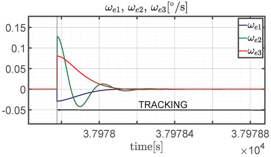
Figure 8. Components of the error angular velocity ${\omega }_{e1}$(t), ${\omega }_{e2}$(t), ${\omega }_{e3}$(t)[°/s] during the fourth tracking interval.

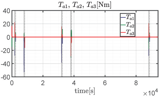
Figure 9. Actual torque components $T_{a_1}$(t), $T_{a_2}$(t), $T_{a_3}$(t)[Nm] during a repetition period.

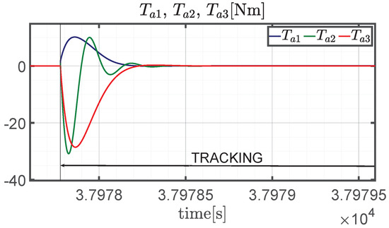
Figure 10. Actual torque components $T_{a_1}$(t), $T_{a_2}$(t), $T_{a_3}$(t)[Nm] during the fourth tracking interval.

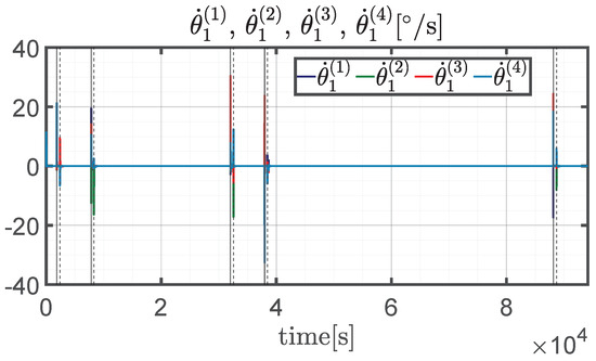
Figure 11. Gimbal angular rates ${\dot{\theta }}_1^{\left(j\right)}$(t)[°/s]; j = 1, …, 4. during a repetition period.

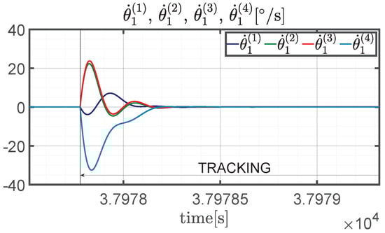
Figure 12. Gimbal angular rates ${\dot{\theta }}_1^{\left(j\right)}$(t)[°/s]; j = 1, …, 4. during the fourth tracking interval.

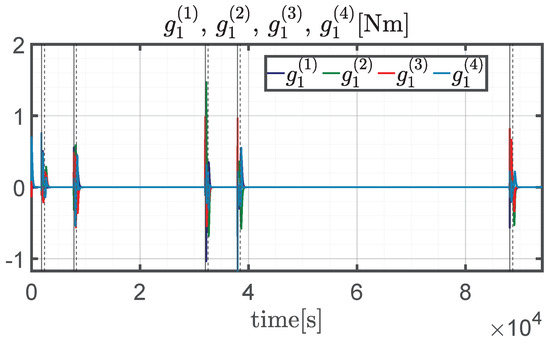
Figure 13. Net motor torques $g_1^{\left(j\right)}$(t); j = 1, …, 4. during a repetition period.

5.3. Monte Carlo Analysis

A Monte Carlo analysis, composed of 100 simulations, is performed for the purpose of ascertaining effectiveness of the control and actuation architecture in nonnominal flight conditions. The final goal is in proving convergence toward the desired attitude in the presence of displacements on the initial conditions, i.e., the spacecraft angular rate and attitude. The latter is randomly generated by assuming an eigenaxis with uniform distribution over the unit sphere, whereas the principal angle has uniform distribution in the interval $[0,\pi ]$,

$$\begin{array}{cc}\hfill & \Phi =\mathcal{U}(0,\pi )\hfill \end{array}$$

(59)

$$\begin{array}{cc}\hfill & \xi =\mathcal{U}(0,2\pi )\hfill \end{array}$$

(60)

$$\begin{array}{cc}\hfill & \varphi ={sin}^{-1}r\hfill \end{array}$$

(61)

$$\begin{array}{cc}\hfill & r=\mathcal{U}(-1,1)\hfill \end{array}$$

(62)

In the preceding relations, symbol $\mathcal{U}$ denotes a uniform distribution, with bounds reported in parenthesis, $\Phi$ is the eigenangle, whereas the two auxiliary angles $\xi$ and $\varphi$ identify the stochastic direction of the eigenaxis $\widehat{a}$ both in the inertial and in the body axes frame, i.e.,

$${\underline{a}}^{(N/B)}={\left[\begin{array}{ccc}cos\varphi cos\xi & cos\varphi sin\xi & cos\xi \end{array}\right]}^T$$

(63)

The initial angular rate components of the spacecraft are assumed to obey a normal distribution, with zero average value and standard deviation equal to 0.5 °/s, i.e.,

$${\omega }_i=\mathcal{N}(0,{\sigma }^2)(i=1,2,3)$$

(64)

where $\mathcal{N}$ is the normal distribution.

The mean value and the standard deviations of two quantities are reported in Table 3, i.e., (a) average value of the pointing error (angle ${\overline{\Phi }}_e$) and (b) average magnitude of the angular velocity error. Figure 14 and Figure 15 illustrate these two quantities for all the simulations. The average pointing error is less than 0.5° for the great majority of the simulations, whereas the average magnitude of the angular velocity error never exceeds $7·{10}^{-3}$ °/s.

Table 3. Downlink: numerical results from the Monte Carlo campaign.

${\overline{\overline{\mathit{\omega }}}}_{\mathit{e}}$[°/s]	${\mathit{\sigma }}_{{\overline{\mathit{\omega }}}_{\mathit{e}}}$[°/s]	${\overline{\overline{\mathbf{\Phi }}}}_{\mathit{e}}$[°]	${\mathit{\sigma }}_{{\overline{\mathbf{\Phi }}}_{\mathit{e}}}$[°]
1.18$·$10${}^{-3}$	8.45$·$10${}^{-4}$	1.93$·$10${}^{-1}$	1.38$·$10${}^{-1}$

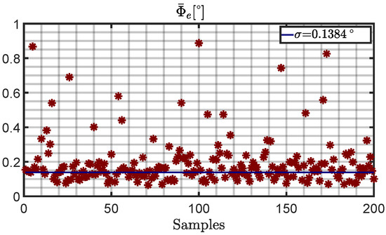
Figure 14. Average pointing error ${\overline{\Phi }}_e$[°] for all simulations of the Monte Carlo campaign.

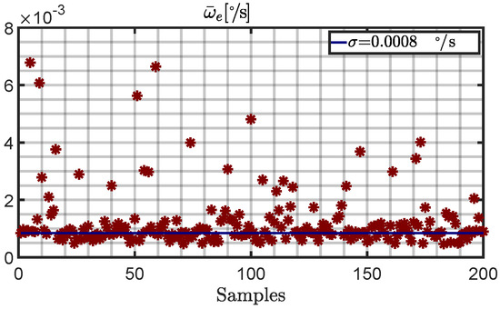
Figure 15. Average magnitude of the angular velocity error ${\overline{\omega }}_e$[°/s] for all simulations of the Monte Carlo campaign.

6. Attitude Maneuvering for Intersatellite Connection

This section considers two satellites placed in two repeating ground-track orbits. When they are mutually visible, the first spacecraft, labeled with S, must point toward the second target satellite, labeled with T. Correct pointing allows establishing an interlink connection for data sharing. Attitude maneuvering is split again in two phases:

• attitude tracking, to point S toward T when the two spacecraft are visible to each other, and
• attitude reorientation, aimed at gaining the correct pointing direction while waiting for the succeeding trajectory arc where T and S are mutually visible.

During attitude tracking, a time-varying attitude and angular velocity are pursued. Instead, attitude reorientation represents a slewing maneuver, with zero angular rate and specified attitude, identified by the constant matrix $R_c$. This corresponds to aligning a specified body axis of S with the direction from S to T, as soon as T becomes visible from S. It is straightforward to recognize that the commanded attitude and the angular velocity are discontinuous across the two trajectory arcs.

In this context, visibility is related to the line of sight between S and T. In particular, let $\theta$ be the angle between the two position vectors; ${\theta }_S$ and ${\theta }_T$ are the angles at vertex O (cf. Figure 16 and Figure 17). The following relations hold:

$$\begin{array}{cc}\hfill & \theta ={cos}^{-1}\left({\displaystyle \frac{{\overrightarrow{r}}_T·{\overrightarrow{r}}_S}{\left|\right|{\overrightarrow{r}}_T\left|\right|\left|\right|{\overrightarrow{r}}_S\left|\right|}}\right)\hfill \end{array}$$

(65)

$$\begin{array}{cc}\hfill & {\theta }_S={cos}^{-1}\left({\displaystyle \frac{r_{\oplus }}{\left|\right|{\overrightarrow{r}}_S\left|\right|}}\right)\hfill \end{array}$$

(66)

$$\begin{array}{cc}\hfill & {\theta }_T={cos}^{-1}\left({\displaystyle \frac{r_{\oplus }}{\left|\right|{\overrightarrow{r}}_T\left|\right|}}\right)\hfill \end{array}$$

(67)

From inspection of Figure 16 and Figure 17 it is apparent that visibility and non-visibility arcs can be distinguished based on these three angles, i.e.,

$$\begin{array}{cc}\hfill & \theta >{\theta }_S+{\theta }_T\to \mathrm{non}\text{-}\mathrm{visibility}\mathrm{arc}\hfill \end{array}$$

(68)

$$\begin{array}{cc}\hfill & \theta <{\theta }_S+{\theta }_T\to \mathrm{visibility}\mathrm{arc}\hfill \end{array}$$

(69)

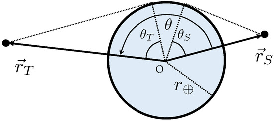
Figure 16. Non-visibility condition ($\theta >{\theta }_S+{\theta }_T$).

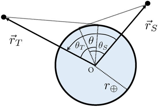
Figure 17. Visibility condition ($\theta <{\theta }_S+{\theta }_T$).

6.1. Commanded Attitude

The spacecraft attitude is referred again to the Earth-centered inertial frame (ECI), associated with vectrix $\underline{\underline{N}}$. The final objective is in defining the commanded attitude, identified by $\underline{\underline{C}}$, in both phases, i.e., tracking and reorientation. In order to achieve correct pointing, a specified spacecraft body axis (i.e., ${\widehat{i}}_c$) must be aligned with the relative position vector that points from S to T.

In the ECI-frame, the position vectors ${\overrightarrow{r}}_S$ and ${\overrightarrow{r}}_T$ can be written in terms of orbit elements, using Equation (41) for both S and T.

The commanded attitude is defined through the following relations:

$$\begin{array}{cc}\hfill & {\widehat{l}}_c={\displaystyle \frac{{\overrightarrow{r}}_T-{\overrightarrow{r}}_S}{\left|\right|{\overrightarrow{r}}_T-{\overrightarrow{r}}_S\left|\right|}}\hfill \end{array}$$

(70)

$$\begin{array}{cc}\hfill & {\widehat{j}}_c={\displaystyle \frac{{\widehat{l}}_c\times {\widehat{c}}_3}{\left|\right|{\widehat{l}}_c\times {\widehat{c}}_3\left|\right|}}\hfill \end{array}$$

(71)

$$\begin{array}{cc}\hfill & {\widehat{k}}_c={\widehat{l}}_c\times {\widehat{j}}_c\hfill \end{array}$$

(72)

For this problem, the commanded attitude reference frame is illustrated in Figure 18. Using Equations (70)–(72), the unit vectors of the commanded attitude are resolved in the ECI-frame, and the rotation matrix that relates the commanded reference frame $\underline{\underline{C}}$ to the inertial reference frame $\underline{\underline{N}}$, denoted with $\underset{C\leftarrow N}{R}$, can be found in closed form.

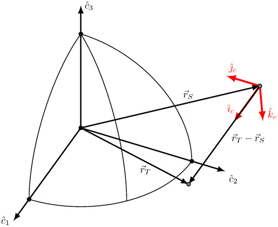
Figure 18. Geometry of the commanded attitude (intersat link).

The time derivative of matrix $\underset{C\leftarrow N}{R}$ is given by

$$\dot{\underset{C\leftarrow N}{R}}=\left({\displaystyle \frac{\partial \underset{C\leftarrow N}{R}}{\partial {{\theta }_{*}}_T}}+{\displaystyle \frac{\partial \underset{C\leftarrow N}{R}}{\partial {{\theta }_t}_T}}\right){\dot{{\theta }_{*}}}_T+\left({\displaystyle \frac{\partial \underset{C\leftarrow N}{R}}{\partial {{\theta }_{*}}_S}}+{\displaystyle \frac{\partial \underset{C\leftarrow N}{R}}{\partial {{\theta }_t}_S}}\right){\dot{{\theta }_{*}}}_S$$

(73)

Equations (47) and (50) still hold in this context. Finally, the derivative of the commanded angular velocity is given by

$${\underline{\dot{\omega }}}_c^{\left(C\right)}=\left({\displaystyle \frac{\partial {\underline{\omega }}_c^{\left(C\right)}}{\partial {{\theta }_{*}}_T}}+{\displaystyle \frac{\partial {\underline{\omega }}_c^{\left(C\right)}}{\partial {{\theta }_t}_T}}\right){\dot{{\theta }_{*}}}_T+\left({\displaystyle \frac{\partial {\underline{\omega }}_c^{\left(C\right)}}{\partial {{\theta }_{*}}_S}}+{\displaystyle \frac{\partial {\underline{\omega }}_c^{\left(C\right)}}{\partial {{\theta }_t}_S}}\right){\dot{{\theta }_{*}}}_S$$

(74)

The preceding developments lead to finding the desired attitude and angular rate in tracking intervals. The desired attitude in reorientation arcs can be found by predicting the inertial position of T at the time when it becomes visible; in this context, ${\underline{\omega }}_c^{\left(C\right)}$ is set to $\underline{0}$, as well as its time derivative.

6.2. Numerical Simulations in Nominal Conditions

The two spacecraft are assumed to be placed in two orbits with identical semimajor axes, eccentricities, and inclinations, set to the values of Section 5.2. Instead, the two orbits have different values of RAAN,

$$\begin{array}{cc}\hfill & {\Omega }_S=0°\hfill \end{array}$$

(75)

$$\begin{array}{cc}\hfill & {\Omega }_T=90°\hfill \end{array}$$

(76)

At the initial time, both satellites are at the ascending node.

Figure 19 depicts $\theta$ and $({\theta }_S+{\theta }_T)$ during a time interval of 10,000 s, in which the two spacecraft are mutually visibible three times. The first and third visibility arc correspond to transits in the North latitudinal regions, the second (shorter) visibility arc is associated with a transit in the South emisphere. The initial attitude conditions are

$$\begin{array}{cc}\hfill & \underline{\omega }\left(t_0\right)={\left[\begin{array}{ccc}0& 0& 0\end{array}\right]}^T\hfill \end{array}$$

(77)

$$\begin{array}{cc}\hfill & \underline{\theta }\left(t_0\right)={\left[\begin{array}{cccc}0& {\displaystyle \frac{\pi }{4}}& {\displaystyle \frac{\pi }{2}}& {\displaystyle \frac{3\pi }{4}}\end{array}\right]}^T\hfill \end{array}$$

(78)

$$\begin{array}{cc}\hfill & \underline{\dot{\theta }}\left(t_0\right)={\left[\begin{array}{cccc}0& 0& 0& 0\end{array}\right]}^T\hfill \end{array}$$

(79)

$$\begin{array}{cc}\hfill & R\left(t_0\right)=\left[\begin{array}{ccc}1& 0& 0\\ 0& -0.1736& -0.9848\\ 0& 0.9848& -0.1736\end{array}\right]\hfill \end{array}$$

(80)

For simulating these attitude maneuvers, Q is set to

$$Q={10}^{-7}{I}_{6\times 6}$$

(81)

The gains used in the numerical simulations are reported in Appendix A.

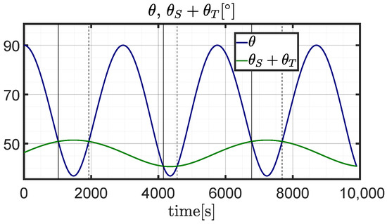
Figure 19. Angles $\theta$, ${\theta }_S$ + ${\theta }_T$(t)[°] during a the entire time interval [0, 10,000] s.

Figure 20 illustrates the eigenangle time history, which provides a clear indication of misalignment. This time history exhibits some spikes immediately after the end of tracking intervals, when S must reorient to point toward the direction where T will appear in the subsequent visibility arc. Instead, during visibility arcs, the eigenangle reaches modest values, e.g., below 0.1°, as shown in Figure 21, referred to the 2nd tracking interval. Figure 22 portrays the time histories of the components of the error angular velocity, which reach again their maximum values at the beginning of reorientation arcs. In contrast, in visibility arcs these components quickly drop to zero, as illustrated in Figure 23. Precision in pointing is testified by the two mean values ${\overline{\Phi }}_{e_i}$ and ${\overline{\omega }}_{e_i}$, defined in Equations (5) and (6),

$$\begin{array}{cc}\hfill & {\overline{\Phi }}_{e_i}=4.90·{10}^{-2}°\hfill \end{array}$$

(82)

$$\begin{array}{cc}\hfill & {\overline{\omega }}_{e_i}=2.60·{10}^{-4}°/\mathrm{s}\hfill \end{array}$$

(83)

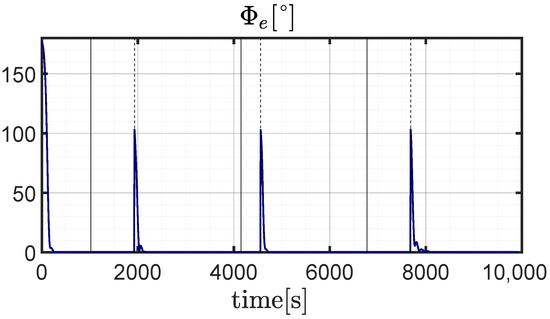
Figure 20. Pointing error ${\Phi }_e$(t)[°] during the entire time interval.

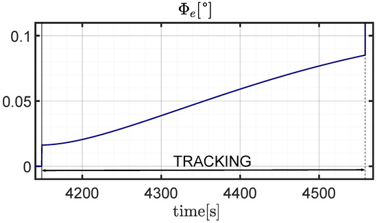
Figure 21. Pointing error ${\Phi }_e$(t)[°] during the second tracking interval.

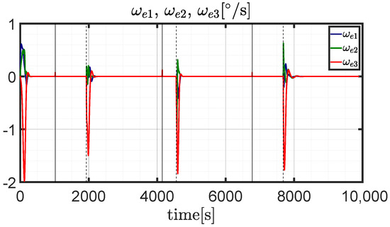
Figure 22. Components of the error angular velocity ${\omega }_{e1}$(t), ${\omega }_{e2}$(t), ${\omega }_{e3}$(t)[°/s] during the entire time interval.

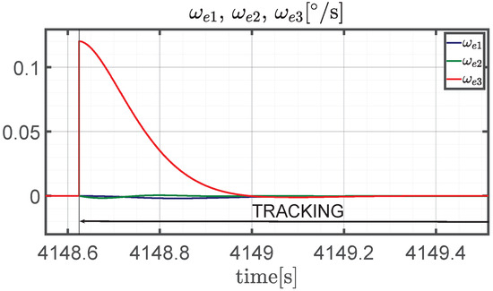
Figure 23. Components of the error angular velocity ${\omega }_{e1}$(t), ${\omega }_{e2}$(t), ${\omega }_{e3}$(t)[°/s] during the second tracking interval.

The actual torque components, depicted in Figure 24 and Figure 25, reach values of order of tens of Nm and component $T_{a3}$ is larger than the other ones. The angular rates of the gimbals are portrayed in Figure 26 and Figure 27, occasionally exceed 20 °/s, and never exceed 35 °/s. The time histories of net motor torques, shown in Figure 28, turn out to be of order of 1 Nm, never exceeding 2 Nm. For the sake of completeness, Figure 29 portrays the time histories of ${\tilde{J}}_{11}$, ${\tilde{J}}_{22}$, ${\tilde{J}}_{33}$, ${\tilde{J}}_{12}$, ${\tilde{J}}_{13}$, and ${\tilde{J}}_{23}$, which represent the displacement of the inertia momenta and products from the respective actual values.

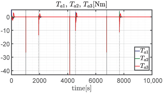
Figure 24. Actual torque components $T_{a_1}$(t), $T_{a_2}$(t), $T_{a_3}$(t)[Nm] during the entire time interval.

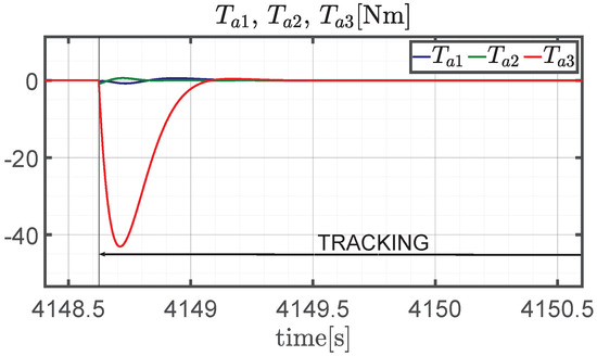
Figure 25. Actual torque components $T_{a_1}$(t),$T_{a_2}$(t),$T_{a_3}$(t)[Nm] during the second tracking interval.

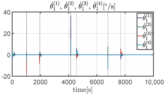
Figure 26. Gimbal angular rates ${\dot{\theta }}_1^{\left(j\right)}$(t)[°/s]; j = 1, …, 4 during the entire time interval.

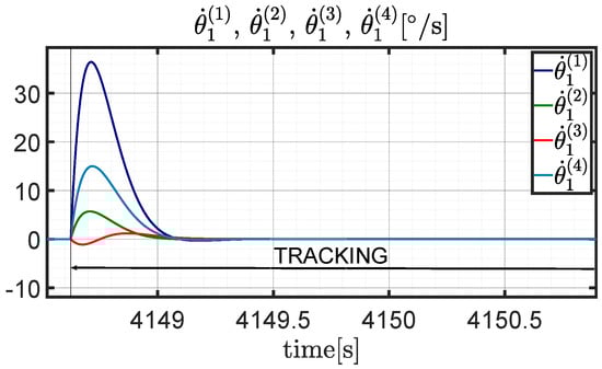
Figure 27. Gimbal angular rates ${\dot{\theta }}_1^{\left(j\right)}$(t)[°/s]; j = 1, …, 4. during the second tracking interval.

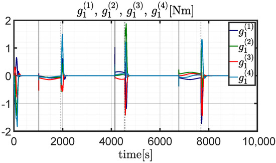
Figure 28. Net motor torques $g_1^{\left(j\right)}$(t); j = 1, …, 4 during the entire time interval.

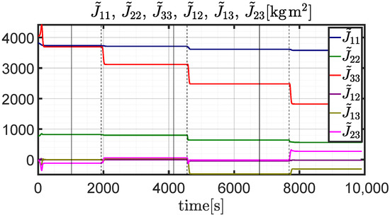
Figure 29. Errors on estimated inertia moments and products ${\tilde{J}}_{11}$(t), ${\tilde{J}}_{22}$(t), ${\tilde{J}}_{33}$(t), ${\tilde{J}}_{12}$(t), ${\tilde{J}}_{13}$(t), ${\tilde{J}}_{23}$(t)[kg ${\mathrm{m}}^2$] during the entire time interval.

6.3. Monte Carlo Analysis

A Monte Carlo analysis is also performed for the interlink attitude maneuvering. The stochastic initial conditions are generated by using the same approach described in Section 5.3. The mean value and the standard deviations of two quantities are reported in Table 4, i.e., (a) average value of the pointing error (angle ${\overline{\Phi }}_e$) and (b) average magnitude of the angular velocity error. Figure 30 and Figure 31 illustrate these two quantities for all the simulations. The average pointing error is less than 0.3° for the great majority of the simulations, whereas the average magnitude of the angular velocity error never exceeds $6·{10}^{-3}$ °/s and is less than $5·{10}^{-4}$ °/s in most cases.

Table 4. Intersat: numerical results from the Monte Carlo campaign.

${\overline{\overline{\mathit{\omega }}}}_{\mathit{e}}$[°/s]	${\mathit{\sigma }}_{{\overline{\mathit{\omega }}}_{\mathit{e}}}$[°/s]	${\overline{\overline{\mathbf{\Phi }}}}_{\mathit{e}}$[°]	${\mathit{\sigma }}_{{\overline{\mathbf{\Phi }}}_{\mathit{e}}}$[°]
3.05$·$10${}^{-4}$	4.51$·$10${}^{-4}$	9.89$·$10${}^{-2}$	6.64$·$10${}^{-2}$

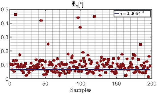
Figure 30. Average pointing error ${\overline{\Phi }}_e$[°] for all simulations of the Monte Carlo campaign.

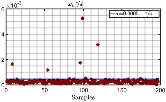
Figure 31. Average magnitude of the angular velocity error ${\overline{\omega }}_e$[°/s] for all simulations of the Monte Carlo campaign.

7. Concluding Remarks

This research addresses the design and numerical testing of an attitude control architecture tailored to precise satellite reorientation and tracking, in two operational scenarios: (a) pointing toward a ground station, for downlink data routing, and (b) pointing toward a companion satellite, for intersatellite data sharing. In each scenario, two distinct phases are identified, i.e., (i) attitude tracking and (ii) reorientation. The related commanded attitude and angular rate are obtained in closed form through geometric analysis. An inertia-free nonlinear attitude control algorithm leads to obtaining a feedback law for the commanded torque components. Actuation is demanded to an array of four single-gimbal control momentum gyroscopes. They are driven through the use of an effective steering law that incorporates singular direction avoidance. Accurate modeling of the actuation devices allows finding the actual torque transferred to the spacecraft, as well as the net motor torque to apply to each device. Both mission scenarios include slewing and tracking phases. Nonlinear attitude control, in conjunction with actuation, leads to obtaining modest values for the misalignment angle and the angular velocity error. The single-gimbal control momentum gyroscopes are effectively steered while remaining within their (safe) operational range, without any saturation, and modest motor torques are needed. Lastly, the numerical simulations, assuming either nominal or nonnominal conditions, prove that the control architecture at hand is rather effective for precise attitude maneuvering, with the final aim of establishing downlink and intersatellite connections for data sharing.

References

- Christensen, C.; Beard, S. Iridium: Failures & successes. Acta Astronaut. 2001, 48, 817–825. [Google Scholar]
- Leopold, R.J. The Iridium communications systems. In Proceedings of the Singapore ICCS/ISITA92, Singapore, 16–20 November 1992; IEEE: New York, NY, USA, 1992; pp. 451–455. [Google Scholar]
- Leopold, R.J. Low-earth orbit global cellular communications network. In Proceedings of the ICC 91 International Conference on Communication Conference Record, Denver, CO, USA, 23–26 June 1991; IEEE: New York, NY, USA, 1991; pp. 1108–1111. [Google Scholar]
- Wiedeman, R.; Salmasi, A.; Rouffet, D. Globalstar-Mobile communications where ever you are. In Proceedings of the 14th International Communications Satellite Systems Conference and Exhibit, Washington, DC, USA, 22 March 1992; p. 1912. [Google Scholar]
- Comparetto, G.; Hulkower, N. Global mobile satellite communications-A review of three contenders. In Proceedings of the 15th International Communications Satellite Systems Conference and Exhibit, San Diego, CA, USA, 28 February–3 March 1994; p. 1138. [Google Scholar]
- Dumont, P. Low earth orbit mobile communication satellite systems: A two-year history since WARC-92. Acta Astronaut. 1996, 38, 69–73. [Google Scholar] [CrossRef]
- Evans, J.V. Satellite systems for personal communications. Proc. IEEE 1998, 86, 1325–1341. [Google Scholar] [CrossRef]
- Del Portillo, I.; Cameron, B.G.; Crawley, E.F. A technical comparison of three low earth orbit satellite constellation systems to provide global broadband. Acta Astronaut. 2019, 159, 123–135. [Google Scholar] [CrossRef]
- Le May, S.; Gehly, S.; Carter, B.A.; Flegel, S. Space debris collision probability analysis for proposed global broadband constellations. Acta Astronaut. 2018, 151, 445–455. [Google Scholar] [CrossRef]
- Roth, M.; Brandt, H.; Bischl, H. Implementation of a geographical routing scheme for low Earth orbiting satellite constellations using intersatellite links. Int. J. Satell. Commun. Netw. 2021, 39, 92–107. [Google Scholar] [CrossRef]
- Qu, Y.; Zhong, X.; Zhang, F.; Tong, X.; Fan, L.; Dai, L. Robust disturbance observer-based fast maneuver method for attitude control of optical remote sensing satellites. Acta Astronaut. 2022, 201, 83–93. [Google Scholar] [CrossRef]
- Wang, H.; Bai, S. A versatile method for target area coverage analysis with arbitrary satellite attitude maneuver paths. Acta Astronaut. 2022, 194, 242–254. [Google Scholar] [CrossRef]
- Ponche, A.; Marcos, A.; Ott, T.; Geshnizjani, R.; Loehr, J. Guidance for autonomous spacecraft repointing under attitude constraints and actuator limitations. Acta Astronaut. 2023, 207, 340–352. [Google Scholar] [CrossRef]
- Zentgraf, P. Non-rest to non-rest reference slews for agile imaging satellites with LQ-minimized angular momentum. In Proceedings of the AIAA 2023-2173, National Harbor, MD, USA, 23–27 January 2023. [Google Scholar]
- Gordon, R.; Ceriotti, M.; Worrall, K. Effects of model fidelity and uncertainty on a model-based attitude controller for satellites with flexible appendages. Acta Astronaut. 2024, 214, 30–45. [Google Scholar] [CrossRef]
- Marshall, M.A.; Pellegrino, S. Slew maneuver constraints for agile flexible spacecraft. J. Guid. Control Dyn. 2023; in print. [Google Scholar]
- Yefymenko, N.; Kudermetov, R. Quaternion models of a rigid body rotation motion and their application for spacecraft attitude control. Acta Astronaut. 2022, 194, 76–82. [Google Scholar] [CrossRef]
- Wie, B.; Barba, P.M. Quaternion feedback for spacecraft large angle maneuvers. J. Guid. Control Dyn. 1985, 8, 360–365. [Google Scholar] [CrossRef]
- Weiss, H. Quaternion-based rate/attitude tracking system with application to gimbal attitude control. J. Guid. Control Dyn. 1993, 16, 609–616. [Google Scholar] [CrossRef]
- Napoli, I.; Pontani, M. A new guidance and control architecture for orbit docking using feedback linearization. In Proceedings of the 72nd International Astronautical Congress, Dubai, United Arab Emirates, 25–29 October 2021. [Google Scholar]
- Sanyal, A.; Fosbury, A.; Chaturvedi, N.; Bernstein, D.S. Inertia-free spacecraft attitude tracking with disturbance rejection and almost global stabilization. J. Guid. Control Dyn. 2009, 32, 1167–1178. [Google Scholar] [CrossRef]
- Weiss, A.; Yang, X.; Kolmanovsky, I.; Bernstein, D.S. Inertia-free spacecraft attitude control with reaction-wheel actuation. In Proceedings of the AIAA Guidance, Navigation, and Control Conference, Toronto, ON, Canada, 2–5 August 2010. [Google Scholar]
- Posani, M.; Pontani, M.; Gasbarri, P. Agile Satellite Attitude Maneuvers for Intersat and Downlink Data Routing. In Proceedings of the 11th International Workshop on Satellite Constellations & Formation Flying, Milan, Italy, 7–10 June 2022. [Google Scholar]
- Hughes, P.C. Spacecraft Attitude Dynamics; Dover Publications: Mineola, NY, USA, 2004. [Google Scholar]
- Derman, H.Ö. 3-Axis Attitude Control of a Geostationary Satellite. Master’s Thesis, Middle East Technical University, Ankara, Turkey, 1999. [Google Scholar]
- Cruz, G.; Yang, X.; Weiss, A.; Kolmanovsky, I.; Bernstein, D.S. Torque-saturated, inertia-free spacecraft attitude control. In Proceedings of the AIAA Guidance, Navigation, and Control Conference, Portland, OR, USA, 8–11 August 2011. [Google Scholar]
- Posani, M.; Pontani, M.; Gasbarri, P. Nonlinear Slewing Control of a Large Flexible Spacecraft Using Reaction Wheels. Aerospace 2022, 9, 244. [Google Scholar] [CrossRef]
- M50 Control Moment Gyroscope (CMG). Available online: https://satcatalog.s3.amazonaws.com/components/6/SatCatalog_-_Honeywell_-_M50_CMG_-_Datasheet.pdf?lastmod=20210708012029 (accessed on 23 October 2023).
- Leve, F.A.; Hamilton, B.J.; Peck, M. A Spacecraft Momentum Control Systems; Springer: Berlin/Heidelberg, Germany, 2015. [Google Scholar]
- Pontani, M. Advanced Spacecraft Dynamics; Edizioni Efesto: Rome, Italy, 2023. [Google Scholar]
- Wie, B. Space Vehicle Dynamics and Control; AIAA Education Series; American Institute of Aeronautics and Astronautics: Reston, VA, USA, 2008. [Google Scholar]
- Schaub, H.; Junkins, J.L. Analytical Mechanics of Space Systems; AIAA Education Series; American Institute of Aeronautics and Astronautics: Reston, VA, USA, 2003; pp. 404–406. [Google Scholar]
Disclaimer/Publisher’s Note: The statements, opinions and data contained in all publications are solely those of the individual author(s) and contributor(s) and not of MDPI and/or the editor(s). MDPI and/or the editor(s) disclaim responsibility for any injury to people or property resulting from any ideas, methods, instructions or products referred to in the content. |
© 2023 by the authors. Licensee MDPI, Basel, Switzerland. This article is an open access article distributed under the terms and conditions of the Creative Commons Attribution (CC BY) license (https://creativecommons.org/licenses/by/4.0/).