Featured Application
Resource and environmental effects of coastal region and background noise.
Abstract
The continuous data from the YL array and four AU stations during the lifetime of the cyclone TOMAS in March 2010 were downloaded from IRIS. By performing frequency-wave number (F-K) analysis on the array data, it was found that the orientation of the maximum energy of the secondary microseisms (0.1~0.5 Hz) was consistent with the movement of TOMAS when the central wind speed reached the typhoon level. The high wind speed of the cyclone could generate secondary microseisms as well as the high swell. However, the large global earthquake can affect the microseismic observations using F-K. The AU stations have a better microseism observation than the YL array, which might be due to the vibrating and tilting of the hydrophone caused by the turbulence. The F-K analysis on microseisms can produce better slowness and back azimuth observations than polarization.
1. Introduction
What appears to be a randomly disturbed noise in the seismic record is actually a permanent and persistent seismic signal generated by ocean activity, which is an important non-traditional seismic signal known as ambient noise.
Ambient noise has a frequency band of about 0.05 Hz to 0.5 Hz and is mainly generated by the energy of oceanic gravity waves [1]. Ambient noise can be divided into two categories based on the frequency at which the energy is concentrated and the mechanism of generation: (1) single-frequency microseisms, known as primary microseisms, with a frequency range from 0.05 to 0.1 Hz [2]; (2) double-frequency microseisms, known as secondary microseisms, with a frequency range from 0.1 to 0.5 Hz [3].
The theory for primary microseisms is nonlinear coupling between the ocean wave and the shoal or shallow water. Seismologists have found that the sources of primary microseisms are mainly shallow marine areas near the coastline. One strong source is off the Atlantic coast [4,5,6,7], and the other two major sources of primary microseisms are along the west coast of the North American continent and in Polynesia in the South Pacific [4,8]. Secondary microseisms are modeled by the theory of linear coupling between two trains of waves with the same frequency and moving toward each other. Seismologists have used the same analysis and research methods to find that their sources are distributed in both coastal regions and pelagic deep-ocean regions [4,9], and that it has seasonal variations in amplitude. On a regional scale, the generation and distribution of secondary microseismic sources are mainly associated with local extreme weather phenomena (e.g., typhoons, cyclones, etc.) [10,11,12].
Harris [13] investigated the P-wave azimuths and slowness from a single, three-component station using the polarization method and from an array using the frequency-wavenumber (F-K) analysis method. He then contrasted the variations between the various data types and processing techniques. His results showed that an array was better at estimating P-wave azimuth than a single station with three components in the presence of noise. Kvaerna and Doornbos [14] discovered that the results generated by an array were more accurate than the slowness measurement from a single station, which is position-dependent and has a higher standard deviation. Henson [15] calculated the azimuth and slowness of 74 teleseismic events and 71 regional seismic events using F-K and found that the noise had no obvious impact on the F-K analysis.
Previous studies have concentrated on the body wave or surface wave energy in seismic events. Secondary microseisms are considered to propagate within the solid Earth mainly in the form of surface waves. Although this part of the microseismic signal is persistent in nature, its energy is much weaker than the surface wave energy in seismic events. In this paper, we use F-K and polarization analysis methods to process the microseisms excited by the cyclone TOMAS and discuss the differences between the two methods, in order to better investigate the characteristics, excitation mechanisms, and propagation of the microseisms excited by cyclones in the Pacific region, so as to predict the path, size, location, and number of cyclones and thus reduce the human casualties and economic losses caused by cyclones.
2. Data
The TOMAS cyclone with a maximum central wind speed of 115 km/h swept over the Pacific nation of Fiji from north to south from 10 March to 17 March 2010. We obtained the central wind speed and track information for TOMAS from the Joint Typhoon Warning Center (JTWC).
The hydrophone array (YL) at 175° E, 21° S in the South Pacific is the closest seismic observation array to cyclone TOMAS. We downloaded 24 h continuous observations for the YL array and the three-component seismic stations in Australia (AU) during the active period of TOMAS from the International Research Institutions for Seismology (IRIS) (Figure 1). The YL array contains 89 instruments, from which 21 stations can obtain observation data at depths ranging from 1000 to 3900 m underwater. Since the F-K analysis method targets plane waves, only eight instruments in the depth range of 2000 to 2600 m were selected to avoid excessive time differences caused by large depth differences. The YL array instrument is the LDED Standard Ocean-Bottom Seismometer, which uses a low-noise amplifier with a velocity response of 0.01–100 s. Four AU stations that use a Streckeisen STS-2 broadband seismometer and are located close to the Pacific region are chosen. This seismometer has a low power and a frequency range beyond the traditional short-period and long-period instruments uses three identical oblique mechanical device sensors to ensure that the horizontal and vertical components are tightly integrated and has a velocity response of 0.1 to 120 s. Due to its wider and comparable frequency range compared to the instrument used in AU stations, the YL array can ensure that we can conduct a comparative study on background noise.
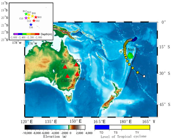
Figure 1.
The location of YL array, green triangles, and four AU stations, red triangles. The circles represent the best tracks of the TOMOS cyclone from JTWC. Inset is the configuration of 8 YL array stations used in the study. TD stands for tropical depression with maximum wind speed 0–34 km/h. TS stands for tropical storm with maximum wind speed 34–63 km/h. TY stands for typhoon with maximum wind speed 63–129 km/h.
In addition, we use ocean-wave data from the global atmospheric reanalysis data (ERA5) provided by the European Centre for Medium-Range Weather Forecasts (ECMWF). ERA5 provides hourly estimates of atmospheric, terrestrial, and oceanic climate variables. The data is accurately gridded into 30 × 30 km and contains 137 layers of atmospheric data. To investigate the fluctuation in swell height and to contrast it with microseism observations, we acquired hourly swell data for the Pacific region throughout the TOMAS cyclone activity period from the ECMWF [16].
3. Methodology
In this paper, frequency-wave number (F-K) [17,18] and polarization analysis [19] are used to study the excitation mechanism of the microseisms generated by TOMAS and its source area.
The F-K method’s fundamental principle is to use Capon’s high-resolution methodology [16] to extract information from the covariance matrix to estimate the slowness and back azimuth of the signal arriving at the array. In order to reduce the effect of the array response on the F-K spectrum by applying station weights. This algorithm is performed under the plane wave assumption by operating on the slowness vector at a time and measuring the energy output. Since different types of seismic waves have different slowness and different source locations can have different back azimuth, F-K analysis is a grid search method in the slowness space. The basic idea is to find the best combination of slowness and back azimuth to maximize energy.
Polarization analysis uses a single-station algorithm to obtain frequency-dependent information from three-component seismic data. Our frequency domain polarization technique has been extensively discussed before [20]. The approach gives information on the noise power and the polarization properties as a function of time and frequency based on the singular value decomposition of the spectral covariance matrix. The polarization properties include the degree of polarization and the direction of arrival at the seismometer. The polarization approach, in contrast to F-K or beamforming analysis, only calculates between different components of a single station.
4. Results
4.1. Results of F-K Analysis
The non-uniform station distribution within the array can cause energy spread and leakage, which can be determined using the array response function (ARF) in the slowness domain. If the stations are evenly spaced, the ARF energy should show a two-dimensional delta function, with the maximum energy in the center and gradually decaying in all directions [21,22]. First, we choose stations based on the array response function, which displays a two-dimensional delta shape of the energy with fewer sidelobes. Only 21 of the 89 sites in the YL array have data, and the range of depth for these 21 stations is 1000 to 3900 m. We chose eight stations with depths between 2000 and 2600 m to reduce the impact of station elevation differences on the F-K analysis. The array response function with a central frequency of 0.25 Hz was obtained (Figure 2). In order to ensure the accuracy of the F-K analysis for secondary microseisms, the ARF composed of eight stations exhibits a virtually two-dimensional delta function distribution with low energy sidelobes located far from the center.
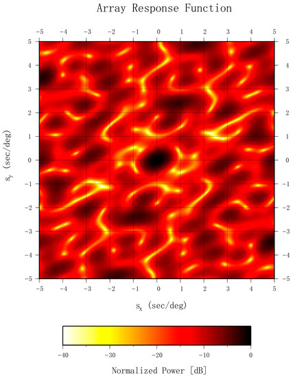
Figure 2.
The array response function of YL array.
After selecting the suitable stations, we performed F-K analysis on the continuous seismic data during the TOMAS cyclone’s active period. The sampling rate of the YL array was 40 points/s. We used a sliding window to analyze hourly continuous data, with each subwindow being 16,384 points (409.6 s) long and overlapping the adjacent subwindow by 50%. Each subwindow was detrended, then filtered using a Hanning window with a bandwidth of 0.1 to 0.5 Hz, the frequency band of the secondary microseisms. During the grid search of the slowness and back azimuth, the beam was formed using fourth root stacking. We normalized the F-K calculation results through the lifetime of TOMAS, then analyzed the relationship between the TOMAS cyclone path, wind speed, ocean swell, and the seismic results (Figure 3).
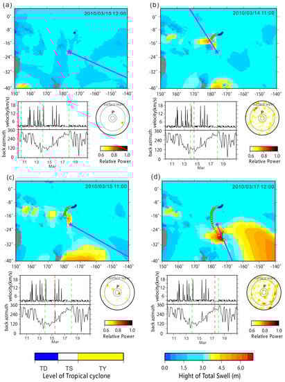
Figure 3.
Results of F-K analysis in the range of 0.1 to 0.5 Hz at four different times during the TOMAS cyclone’s lifetime period (a–d). The comparison between the F-K result, the location of the cyclone center, and the swell is shown in the upper portion of 3 (a–d). The purple star is the location of the YL array, and the purple ray is the back azimuth from F-K. The circles are the locations of the centers of TOMAS. The back azimuth and velocity of the peak energy from F-K as a function of time are shown in the lower left part. The beginning and ending times when the F-K results have a good correlation with the cyclone are marked by the green dashed lines at 21:00 on 13 March and 03:00 on 18 March. The red dashed line marks the corresponding time of the upper portion. The lower right portion is the slowness measurement at the corresponding time of the upper portion from F-K. The P wave slowness and surface wave slowness are marked as concentric circles.
On 10 March 2010, at 12:00 am, TOMAS was still in the tropical depression state (Figure 3a), with a central wind speed of only 25 km/h located north of the array. The cyclone’s energy at this time was insufficient to have a significant dragging effect on the seawater along the cyclone’s path, and the swell heights given by ERA5 were below 2 m. Although the peak energy of the F-K analysis has a surface wave velocity (3.59 km/s), its orientation is east–southeast rather than the direction of the cyclone TOMAS. Since there is a wide area with little land in the South Ocean, the region has high wave heights from a global perspective, and the seasonal variation in wave height is not significant. This feature makes the South Ocean one of the main sources of microseismic signals [23,24]. The results of F-K analysis at that moment probably came from the South Ocean. On 14 March, at 11:00 am, TOMAS upgraded to typhoon level with a maximum central wind speed of 100 km/h and was the northwest of the array (Figure 3b). The swell data from ERA5 indicated that the core of TOMAS is moving along with a high swell of roughly 6 m. The results of the F-K analysis showed that the secondary microseismic energy traveled at the surface wave velocity and had a direction that pointed to TOMAS and the high swell area. On 17 March, around 12:00 am, TOMAS still maintained typhoon level and had moved to the southeast of the array. The high swell area followed the cyclone’s movement. The results of the F-K analysis showed that the energy with surface wave velocity pointed to the cyclone’s center, which was accompanied by the high swell (Figure 3d). The peak energy of secondary microseisms from the F-K analysis was propagating at surface wave velocity (about 3 km/s), and its back azimuth varied from 120° to 300° (Figure 3). This change in the back azimuth closely matched TOMAS’ moving path, which swept roughly 24° (almost 2700 km) from north to south between 13 March and 17 March. According to the back azimuth and velocity, the secondary microseisms were generated by the high swell that closely followed the center of TOMAS when the cyclone maintained the typhoon level, which was where the wind speed was the strongest and where opposing waves were produced to generate secondary microseisms.
When a large global earthquake occurs, the secondary microseism period is dominated by the surface wave energy from the larger earthquake rather than the signal from the ocean. At 11:08:32 on 15 March, an earthquake with magnitude 6.2 occurred in Chile, 73.49° W, 35.85° S, South America. On 15 March, about 11:00 am, even though TOMAS was moving towards the YL array with the central wind speed at typhoon level, the energy in the secondary microseism period had P wave velocity and pointed to the southeast direction of the array, which was the direction of the Chile earthquake, instead of the velocity of the microseism and the direction of the cyclone (Figure 3c).
4.2. Results of Polarization Analysis
We applied polarization analysis to the three-component, hour-long continuous data for the YL array and four AU stations. Firstly, the instrument response was removed, and two differentiations were performed to obtain the ground acceleration. Then the hour-long data was divided into 27 sliding windows, each with a length of 8192 samples (204.8 s) and a sliding volume of 5096 points (127.4 s). The overlap rate between two sub-windows was 62%. Each sub-window was detrended, filtered with a Hanning window, and applied fast Fourier-transform (FFT) to perform a 3 × 3 spectral covariance matrix. Finally, an overall spectral covariance matrix of the hour-long data was obtained by averaging 27 spectral covariance matrices. The eigenvalue and eigenvector of the overall spectral covariance matrix represented the polarization of the noise over the one-hour period.
The results of the polarization analysis showed that the secondary microseism energies from the YL array were significantly higher than those from four AU stations, regardless of the level of the cyclone wind speed or the distance between the station and the cyclone center (Figure 4). A similar result had been found for the comparison between the ocean bottom seismometers and land stations [25,26,27]. This could be due to the different location of the instrument. Since the YL array was in the water, it was exposed to swell propagating from multiple source regions and ended in a broader secondary microseism frequency range and higher energies [28]. As the secondary microseism energy is mainly radiated as Rayleigh wave, which attenuates very quickly when it travels through the shoreline to the continent’s crust, four AU stations, located on land approximately 3000 km away from the YL array, exhibited substantially lower secondary microseism energy than the hydrophones.

Figure 4.
Back azimuth, black bar, and power spectral density from polarization analysis for YL and AU at four different times. (a) 10 March 2010 12:00; (b) 14 March 2010 18:00; (c) 15 March 2010 11:00; (d) 17 March 2010 12:00. Inset upper left is the PSDs for YL, black line, and AU stations, the dashed line. Inset circle is the zoom-in to show the back azimuths for YL array.
With the north–south motion of TOMAS, the direction of the secondary microseism from four AU stations slightly shifted from northeast to southeast (Figure 4). In contrast, none of the directions from the YL array showed this change. Several peaks in the secondary microseism period caused by the swell propagating from multiple source regions would have an impact on the direction measurement. The vibrating and tilting of the hydrophone caused by the turbulence could be another factor contributing to the inaccurate direction measurement of the polarization analysis since the effect of this noise had not been removed by the method [29].
4.3. Comparison of Direction Results
We acquire the difference, between the direction measurements, , from the two analysis methods and the actual azimuth, of the cyclone center in relation to the location of YL in order to more easily compare the direction results from F-K and polarization analysis:
A correlation coefficient C is defined as:
The range of C is between −1 and 1. After that, the correlation coefficients C obtained from the F-K and polarization analyses within 0.1~0.5 Hz are averaged.
The F-K analysis had a high correlation with the azimuth of the cyclone center relative to the array (Figure 5), especially between 13 March and 17, when the cyclone wind speed reached typhoon level. Before 13 March, when the cyclone had low wind speeds and was far away from the array, the azimuth from the F-K analysis pointed to the South Ocean, which has high secondary microseism energy throughout the year due to less land and strong atmospheric movement. This resulted in a negative correlation coefficient. The azimuth results from the polarization analysis did not show a clear correlation with the location of the cyclone throughout the cyclone’s lifetime.
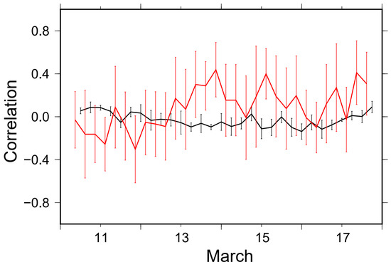
Figure 5.
Correlation analysis for energy in between 0.1 and 0.5 Hz. Red: the F-K analysis results. Black: the polarization results. The error bar is the standard deviation.
Harris [13] analyzed seismic signals using a seismic array and a single station with three components and provided the azimuth estimate error:
for an array with vertical elements and
for a single station with a three-component station, where SNR stands for the signal-to-noise ratio, is the radius of the array, λ is the wavelength of the incident wave, is the azimuth angle from the north, and is the angle of incidence from the vertical. At this point, it is apparent that the azimuth error is smaller than that of a single station with three components.
Overall, the F-K analysis gave better results for azimuth estimation than polarization analysis. The fact that polarization analysis used a single-station approach while F-K employed multi-stations could be the cause of this significant difference. The constraint of the array was stronger than that of a single three-component station, which led to a more accurate estimation of the direction. Additionally, at a particular signal-to-noise ratio, the F-K was unaffected by noise, whereas the polarization analysis was also impacted by additional polarization features [13].
5. Conclusions
We processed continuous seismic data from the YL array and four AU stations using both F-K and polarization analysis and looked at the relationships between secondary microseisms, cyclones, and swell, as well as the differences between the two approaches. The results demonstrated that the direction of the secondary microseism did not closely match the route of the cyclone when the central wind speed was slow. However, due to the high wind speed, when the cyclone level reached typhoon level, the high swell area traveled along the cyclone motion and produced the secondary microseismic signal that can be observed on the seismographs. The F-K based on the multi-station approach is more accurate in estimating the direction than polarization analysis based on the single-station method. A big global earthquake could affect the measurement using F-K. The polarization results from the AU stations are better than the results from the hydrophone array.
Author Contributions
Y.X. and S.W. designed the study, performed the calculation, and interpreted the results. Y.X. and C.X. wrote the manuscript. A.L. provided comments to improve the manuscript. All authors discussed the results and interpretations and participated in writing the paper. All authors have read and agreed to the published version of the manuscript.
Funding
This work was supported by the National Science Foundation of China under awards 41564003,41964001 and the Xing Dian Talent Plan of Yunnan Province.
Institutional Review Board Statement
Not applicable.
Informed Consent Statement
Not applicable.
Data Availability Statement
Data are available at www.iris.edu; www.ecmwf.int/ (accessed on 10 November 2022).
Acknowledgments
We are thankful to the anonymous reviewers for their constructive comments that allowed us to improve this manuscript.
Conflicts of Interest
All the authors listed certify that they have no involvement in any organization or entity with any financial interest (including honoraria; educational grants; participation in speakers’ membership, bureaus, consultancies, stock ownership, employment, or other equity interest; and patent-licensing arrangements or expert testimony) or nonfinancial interest (including professional or personal relationships, knowledge or beliefs, affiliations) in the subject materials or matter discussed.
References
- Banerji, S.K. Theory of microseisms. Proc. Indian Acad. Sci. Sect. A 1935, 1, 727–753. [Google Scholar] [CrossRef]
- Hasselmann, K. A statistical analysis of the generation of microseisms. Rev. Geophys. 1963, 1, 177–210. [Google Scholar] [CrossRef]
- Longuet-Higgins, M.S. A Theory of the Origin of Microseisms. Philos. Trans. R. Soc. Lond. 1950, 243, 1–35. [Google Scholar] [CrossRef]
- Cessaro, R.K. Sources of primary and secondary microseisms. Bull. Seismol. Soc. Am. 1994, 84, 142–148. [Google Scholar] [CrossRef]
- Friedrich, A.; Krüger, F.; Klinge, K. Ocean-generated microseismic noise located with the Gräfenberg array. J. Seismol. 1998, 2, 47–64. [Google Scholar] [CrossRef]
- Juretzek, C.; Hadziioannou, C. Where do ocean microseisms come from? A study of Love-to-Rayleigh wave ratios. J. Geophys. Res. Solid Earth 2016, 121, 6741–6756. [Google Scholar] [CrossRef]
- Kimman, W.P.; Campman, X.; Trampert, J. Characteristics of Seismic Noise: Fundamental and Higher Mode Energy Observed in the Northeast of the Netherlands. Bull. Seismol. Soc. Am. 2012, 102, 1388–1399. [Google Scholar] [CrossRef]
- Traer, J.; Gerstoft, P.; Bromirski, P.D.; Shearer, P.M. Microseisms and hum from ocean surface gravity waves. J. Geophys. Res. Atmos. 2012, 117, 11307. [Google Scholar] [CrossRef]
- Tian, Y.; Ritzwoller, M.H. Directionality of ambient noise on the Juan de Fuca plate: Implications for source locations of the primary and secondary microseisms. Geophys. J. Int. 2015, 201, 429–443. [Google Scholar] [CrossRef]
- Gerstoft, P.; Fehler, M.C.; Sabra, K.G. When Katrina hit California. Geophys. Res. Lett. 2006, 33, L17308. [Google Scholar] [CrossRef]
- Chi, W.-C.; Chen, W.-J.; Kuo, B.-Y.; Dolenc, D. Seismic monitoring of western Pacific typhoons. Mar. Geophys. Res. 2010, 31, 239–251. [Google Scholar] [CrossRef]
- Sufri, O.; Koper, K.D.; Burlacu, R.; de Foy, D. Microseisms from Superstorm Sandy. Earth Planet. Sci. Lett. 2014, 402, 324–336. [Google Scholar] [CrossRef]
- Harris, D.B. Uncertainty in Direction Estimation: A Comparison of Small Arrays and Three-Component Stations; U.S. Department of Energy Office of Scientific and Technical Information: Oak Ridge, TN, USA, 1982. [CrossRef]
- Kvaerna, T.; Doornbos, D. An integrated approach to slowness analysis with array and three-component stations. NORSAR Semiannu. Technucal Summ. 1986, 2, 60–69. [Google Scholar]
- Suteau-Henson, A. Estimating azimuth and slowness from three-component and array stations. Transl. World Seismol. 2000, 80, 1987–1998. [Google Scholar] [CrossRef]
- ECMWF. Available online: https://www.ecmwf.int/ (accessed on 29 November 2022).
- Capon, J. High-resolution frequency-wavenumber spectrum analysis. Proc. IEEE 1969, 57, 1408–1418. [Google Scholar] [CrossRef]
- Koper, K.D.; de Foy, B.; Benz, H. Composition and variation of noise recorded at the Yellowknife Seismic Array, 1991–2007. J. Geophys. Res. Solid Earth 2009, 114. [Google Scholar] [CrossRef]
- Park, J.; Vernon, F.L.; Lindberg, C.R. Frequency dependent polarization analysis of high-frequency seismograms. J. Geophys. Res. Solid Earth 1987, 92, 12664–12674. [Google Scholar] [CrossRef]
- Koper, K.D.; Hawley, V.L. Frequency dependent polarization analysis of ambient seismic noise recorded at a broadband seismometer in the Central United States. Earthq. Sci. 2010, 23, 439–447. [Google Scholar] [CrossRef]
- Rost, S.; Thomas, C. Array seismology: Methods and applications. Rev. Geophys. 2002, 40, 2-1–2-27. [Google Scholar] [CrossRef]
- Xu, Y.; Koper, K.D.; Sufri, O.; Zhu, L.; Hutko, A.R. Rupture imaging of the Mw 7.9 12 May 2008 Wenchuan earthquake from back projection of teleseismic P waves. Geochem. Geophys. Geosystems 2009, 10, Q04006. [Google Scholar] [CrossRef]
- Stutzmann, E.; Schimmel, M.; Patau, G.; Maggi, A. Global climate imprint on seismic noise. Geochem. Geophys. Geosystems 2009, 10, Q11004. [Google Scholar] [CrossRef]
- Hillers, G.; Graham, N.; Campillo, M.; Kedar, S.; Landès, M.; Shapiro, N. Global oceanic microseism sources as seen by seismic arrays and predicted by wave action models. Geochem. Geophys. Geosystems 2013, 13, Q01021. [Google Scholar] [CrossRef]
- Montagner, J.-P.; Karczewski, J.-F.; Romanowicz, B.; Bouaricha, S.; Lognonne’, P.; Roult, G.; Stutzmann, E.; Thirot, J.-L.; Brion, J.; Dole, B.; et al. The French Pilot Experiment OFM-SISMOBS: First scientific results on noise level and event detection. Phys. Earth Planet. Inter. 1994, 84, 321–336. [Google Scholar] [CrossRef]
- Romanowicz, B.; Stakes, D.; Montagner, J.P.; Tarits, P.; Uhrhammer, R.; Begnaud, M.; Stutzmann, E.; Pasyanos, M.; Karczewski, J.-F.; Etchemendy, S.; et al. MOISE: A pilot experiment towards long term sea-floor geophysical observatories. Earth Planets Space 1998, 50, 927–937. [Google Scholar] [CrossRef]
- Webb, S. Broadband seismology and noise under the ocean. Rev. Geophys. 1998, 36, 105–142. [Google Scholar] [CrossRef]
- Aster, R.C.; McNamara, D.E.; Bromirski, P.D. Multidecadal Climate-induced Variability in Microseisms. Seismol. Res. Lett. 2008, 79, 194–202. [Google Scholar] [CrossRef]
- Webb, S.C. Long-period acoustic and seismic measurements and ocean floor currents. IEEE J. Ocean. Eng. 1988, 13, 263–270. [Google Scholar] [CrossRef]
Disclaimer/Publisher’s Note: The statements, opinions and data contained in all publications are solely those of the individual author(s) and contributor(s) and not of MDPI and/or the editor(s). MDPI and/or the editor(s) disclaim responsibility for any injury to people or property resulting from any ideas, methods, instructions or products referred to in the content. |
© 2023 by the authors. Licensee MDPI, Basel, Switzerland. This article is an open access article distributed under the terms and conditions of the Creative Commons Attribution (CC BY) license (https://creativecommons.org/licenses/by/4.0/).