Article

Effective Microorganisms and Olive Mill Wastewater Used as Biostimulants to Improve the Performance of Tanacetum balsamita L., a Medicinal Plant

1
Institute of BioEconomy, National Research Council (CNR-IBE), Via Madonna del Piano n. 10, Sesto Fiorentino, - 50019 Florence, Italy
2
Research Institute on Terrestrial Ecosystems, National Research Council (CNR-IRET), Via Madonna del Piano n. 10, Sesto Fiorentino, 10-50019 Florence, Italy
3
National Biodiversity Future Center (NBFC), Piazza Marina n. 61, 90133 Palermo, Italy
*
Authors to whom correspondence should be addressed.
Appl. Sci. 2023, 13(2), 722; https://doi.org/10.3390/app13020722
Submission received: 5 December 2022 / Revised: 28 December 2022 / Accepted: 29 December 2022 / Published: 4 January 2023
(This article belongs to the Special Issue Knowledge-Based Biotechnology for Food, Agriculture and Fisheries)

Abstract

:
The use of biostimulants and/or biofertilizers has acquired considerable importance and can contribute to the sustainable management agriculture, reducing the use of chemical fertilizers, pesticides, and water. This study aims to assess the effects of Effective Microorganisms (EM) and Olive Mill Wastewater (OMW) on the growth, photosynthetic performance and polyphenols content of the medicinal plant Tanacetum balsamita. The EM and OMW were used at two dilution rates. The EM was added to 5% v/v and 10% v/v, while OMW was added to 2.5% v/v and 5% v/v in plants at the early growth stage. After 75 days of treatment, all the treated plants had a leaf number and leaf area almost 2-fold higher than in the Control plants. Moreover, the treatments, at all the concentrations applied had a positive effect on the photosynthetic activity, with an improvement both in terms of the quantum yield of photosynthesis and electrons transport efficiency. The best photosynthetic and growth performances in the treated plants coincided with the higher production of phenolic compounds; indeed, after 75 days, the content of chlorogenic acid, caffeic acid, and isochlorogenic acid was even 2-fold of the Control plants. Also, rutin content was 1.28–1.50-fold respect to the Control extracts. The highest phenolic compound content was reflected by the highest antiradical activity, found in the extracts of the treated plants. The effectiveness of EM to increase the growth and quality of plants and in particular, the potential use of OMW on the cultivated crop was confirmed to this study.

1. Introduction

Management strategies in conventional farming systems are strongly characterized by an increased use of fertilizers and pesticides, an excessive use of water irrigation and, in general, an establishment of intensive crop cultivation systems. This context led cropping systems to be less resilient to changing environmental conditions, negatively affected soil quality as well as resulted in serious risks to human health and the environment. In recent years, efforts have been directed toward sustainable farming systems to reduce inputs of chemical fertilizers, pesticides, and water and achieve the goal of an economically viable and environmentally friendly agricultural production system. Among sustainable techniques, the use of biostimulants and/or biofertilizers is considered a new and environmentally friendly agricultural practice that satisfies both crop intensification and environmental protection. A plant biostimulant is any substance or microorganism applied to plants that enhances nutrition efficiency, biotic and abiotic stress tolerance, and/or crop quality. The use of biostimulants may also increase plant productivity. By extension, with the name “plant biostimulants” could be also designated commercial products containing mixtures of such substances and/or microorganisms [1] and this definition can also include the synthetic microbial consortium also called Effective Microorganisms (EM) and Olive Mill Wastewater (OMW). Generally, EM consists mainly of photosynthetic bacteria, lactic acid bacteria, yeast [2] and it is a registered trademark and a brand name owned by EM Research Organization (EMRO). This microbial consortium could increase organic matter and provide nutrients, thus being an alternative sustainable practice in sustaining plant production without other external inputs such as chemical fertilizers and pesticides and without increasing excessive costs [3,4]. On the other hand, OMW could represent a strategic resource in integrated agricultural system management, since it would meet the two-fold objectives of eliminating olive oil waste and using it beneficially to improve soil fertility [5,6]). The characteristics of OMW are variable and depend on the geographic site, plant cultivar and maturity, climatic conditions, cultivation/processing procedures, and oil extraction processes [7,8]. Commonly OMW has high chemical and biological oxygen demand as well as high amounts of total phenols, carbohydrates, polysaccharides, fatty acids, polyalcohols, pectins, and tannins [9,10] that represent a lignin-like structure and constitute the most resistant fraction of this waste stream [11]. OMW usually has a high level of toxicity for the presence of various phenolic compounds, but with appropriate measures and dilutions can be used in agriculture for plants cultivation [12]. The high-polluting power of OMW is related to the presence, in this wastewater, of a high concentration of organic compounds and phenolic acids which confer dark color and low pH. These characteristics make OMW toxic if disposed into the soil, because it can alter the microbial soil composition and its structure, with strong impact to the environment. In this study the effect of the application of EM and OMW on Tanacetum balsamita L. was assessed. Tanacetum balsamita L. (Chrysantenum balsamita L., Balsamita major Desf., Balsamita vulgaris Willd.; Asteraceae family) is a medicinal perennial plant species native of Southern Europe and Western Asia, and it is also known as costmary. Its first botanical description was carried out in the 9th Century by monks who classified all the officinal plants in their gardens [13]. Due to its strong mint-like aroma and bitter taste, it is used to aromatize foods, cakes, drinks and to prepare potpourri [14]. However, the use of costmary as a medical herb is reported in Europe between the 16th and 18th Centuries and in traditional and modern medicine as an antipyretic, laxative, diuretic, digestive, antiseptic, astringent, cardiotonic and for treating burns and insect stings [15,16,17,18]. Its beneficial properties have been attributed to different substances present in the plant, specifically essential oil, and phenolic compounds which are the most abundant antioxidant compounds in the leaves of Tanacetum balsamita [19]. In the sight of these findings, the role of this officinal plant has been revalued and it has been considered in different forms (i.e., aqueous extracts, essential oil) for different uses [19,20]. A present challenge is to find new sustainable (bio)technologies (i.e., EM, OMW) that could increase the production or the phenolic content. In this context, the aim of the present research is to assess the effects of EM and the suitability of OMW on the growth and physiological parameters of Tanacetum balsamita so as to improve the production and quality plants and to contribute a sustainable agronomic application.

2. Materials and Methods

2.1. Experimental Setup

On April 2019, clonal plants of the same age of costmary (Tanacetum balsamita), with average fresh weight of 10.5 g, were transplanted, one in each pot (Ø = 20 cm; h = 20 cm) filled with a commercial substrate (Vigorplant Lodi, Italia) generally used in organic farming (pH = 7; electric conductivity = 0.4 dS m 1 ; total porosity = 87%) and placed under a black polyethylene net (net hole 1.4 × 1.4 mm) with 40% shading intensity in the nursery area of the Italian National Research Council, in Central Italy (Sesto Fiorentino; lat. 43°49 04.2 N; lon. 11°12 06.6 E; 55 m a.s.l.). No chemical fertilizers were added to the plants. The plants were treated with EM, activated in dilution 1:100 [21] provided by CREA-OF (Pescia, Italy) or with OMW (Table A1), provided by a Tuscan oil mill, working with a three-phase process (Pieralisi, Firenze, Italy). OMW was left to settle for a week, at 4 °C, in the dark, to let the solid fraction to deposit in the bottom and the supernatant was used for the treatment.
The treatments were performed by diluting stock solutions with tap water as follows: O1 (OMW 2.5% v/v); O2 (OMW 5% v/v); E1 (EM 5% v/v); E2 (EM 10% v/v); only water (Control). The EM and OMW concentrations applied are in agree with the literature [21,22,23]. Five pots per replicate were arranged in a randomized complete block design with three replications per treatment for a total of fifteen plants per treatment. The pot plants were manually irrigated every 15 days with 1 L of water (Control) or treatment solution to maintain the substrate water content near the field capacity. The experiment ended after 75 days after transplant (DAT), at the balsamic time (at the end of springtime, in June, at this latitude) [24]. Climate conditions were continuously monitored by a weather station (Decagon Em50; Decagon Devices Inc., Pullman, WA 99163, USA). The average minimum and maximum temperatures recorded in the period were 12.95 °C and 25.06 °C, respectively, and the mean relative humidity was 65%. The leaves were collected at intervals: date of data collection reported 15th April (T0), 15th May (T1), 15th June (T2) and 30th June (T3).

2.2. Biometric Parameters: Plant Growth and Trichome Density Analysis

Destructive evaluations were performed on 30 June 2019, at 75 DAT (T3). The following biometric parameters were assessed: leaves number (LN); fresh leaves (FWL), root (FWR), and total (FWT) weight; dry leaves (DWL), root (DWR), and total weight (DWT). All the dry weights occurred after oven drying at 75 °C until a constant weight was reached. Leaf area (LA) was determined on each leaf by image analysis (NIS Elements D 4.00); Specific Leaf Area (SLA; cm 2 g 1 ) was calculated as leaf area/leaf dry mass; Leaf Weight Ratio (LWR; g g 1 ), calculated as DWL/DWT, and leaf area ratio (LAR; cm 2 g 1 ) as S L A × L W R . The Relative Growth Rate (RGR) index was determined according to the equation:
R G R = ln ( D W F ) ln ( D W 0 ) T F T 0
where ln is the natural logarithm, DW0 is the dry mass of the plant at the beginning (T0) and DWF is the dry mass of the plant at the end (TF) of the experiment. The RGR was calculated to leaves and roots. For trichomes density, leaves samples were mounted on aluminum sample-holder stubs, sputtered with silver (Emitech K575X, Emitech Ltd., Ashford, UK), and examined using a GAIA 3 electron microscope (Tescan, Brno, Czech Republic) at 20 KV. Glandular and non-glandular trichomes density (number of trichomes per mm 2 ) were evaluated. All the counts were performed on the central part of the leaf. The histochemical and confocal laser scanning microscopy observations of trichomes were performed on fresh young leaves of Tanacetum balsamita sectioned by hand. The obtained sections were stained with Nadi reagent [25] to detect terpenes. Using a TCS SP8 confocal microscope (Leica Microsystems CMS GmbH, Mannhein, Germany) leaf cross sections were observed. Laser excitation at 405 nm was used to acquire hydroxycinnamate fluorescence (over the 415–480 nm emission spectral band).

2.3. Nutrient Analysis in Leaves

Total N was obtained by dry combustion of dry plant material by using a NA 1500 CHNS Analyser (Carlo Erba, Cornareto, Milano, Italy). Nitrates were determined as described by Cataldo et al. [26]. For K, Mg, Ca, Na, and P-PO4 content determinations, dry shoot samples were wet digested in a mixture of nitric and perchloric acids HNO 3 : HCIO 4 = 5:2 v/v at 230 °C for 1 h. Atomic absorption spectrometry was used to quantify K, Mg, Ca and Na, while spectrophotometry (Evolution™300 UV-Vis Spectrophotometer, Thermo Fisher Scientific Inc., Waltham, MA, USA) was employed for P determination using the molybdenum blue method.

2.4. Chlorophyll a Fluorescence Transient and JIP-Test Parameters

At T0, T1, T2, and T3 the chlorophyll a fluorescence transients were recorded with a Handy-PEA (Hansatech Instruments Limited, Norfolk, UK) on 30 min-dark-adapted leaves then illuminated with continuous light (650 nm peak wavelength, 3500 μ mol photons m 2 s 1 light intensity) provided by light-emitting diodes (LEDs). Each chlorophyll a fluorescence induction curve was analyzed using Biolyzer HP 3 software version 3.03 (Bioenergetics Laboratory, University of Geneva, Switzerland) following the so-called JIP-test [27]. Normalization of the chlorophyll fluorescence data on both F0 and Fm was used, with the transient calculated as relative variable fluorescence V t = F t F 0 F m F 0 , to facilitate the comparisons among the samples [28]. The following parameters (JIP-test parameters), calculated from the fluorescence measurements, were considered: M o = 4 F 300 μ s F 0 F m F 0 , corresponding to the net rate of the reaction center closure; V J = F J F 0 F m F 0 , indicating the level of Quinone A (QA) reduction. The parameters describing the flux ratio were calculated according to Appenroth et al. [29] as follows: F v F m , the maximum quantum yield of PSII for primary photochemistry, ϕ E o = F v F m × Y o , the quantum yield of electron transport.

2.5. Total Polyphenolic Content and Individual Phenolic Determination

Polyphenols were identified by comparing the retention time and the spectrum with the standards, HPLC grade (Sigma-Aldrich). The quantification was obtained using the calibration curve made with the relative standards. Neochlorogenic and chlorogenic acid, gallic acid, Folin-Ciocalteu reagent, and other chemicals used were purchased from Sigma Chemical Co. The total polyphenolic content in the leaves at T0, T1, T2, and T3 was analyzed. Leaves was lyophilised (ALPHA 1–4 LD freeze dryer; Martin Christ, Osterode am Harz, Germany), homogenised and frozen at 80 °C prior to subsequent analyses. For the extraction of phenolic compounds from leaves, 10 mL of methanol:water solution (80:20 v/v) was added to 100 mg of lyophilized leaf material and sonicated with a probe inserted into the liquid suspension (MSE 100-Watt ultrasonic disintegrator, Cat. N.7100) for 1 min. The tubes containing the samples were put in ice during the sonication.
The volume was adjusted to 25 mL. To eliminate the carotenoids and the chlorophylls interferences, all the extracts were washed by adding petrol 1:1 v/v and then centrifuged at 4000× g for 5 min to recover the methanol fraction. The total phenol assay was performed using the Folin-Ciocalteau reagent as described by Luthria et al. [30]. The Folin Ciocalteau reagent was used as supplied by the company. The reaction mixture was freshly prepared every time. The absorbance of the colored reaction product was read at 730 nm, using a Varian UV-Visible spectrophotometer Cary 50 Scan spectrophotometer (Agilent Technologies, Palo Alto, CA, USA). The results were expressed as µg of gallic acid equivalent ( μ g GAE g 1 ). The total phenolic compound extractions were performed in triplicate.

2.6. Phenolic Compounds Determination in Leaves Extracts

HPLC-DAD analyses for identification and quantification of the individual phenolic compounds were performed according to Romani et al. [31] on the previously described methanol extracts. For polyphenolic identification and quantification, the standards by Sigma-Aldrich of HPLC grade were used. Analysis was conducted with a Varian multisolvent pump ProStar 210 (Agilent Technologies, Palo Alto, CA, USA), coupled with a photodiode array detector Varian ProStar 335 (Agilent Technologies, Palo Alto, Ca, USA). For the separation, the analysis was performed with a Phenomenex Kinetex Phenyl-Hexyl 100 A 150 × 4.6 mm reverse-phase C18 column with an identical pre-column, at 25 °C. The eluent was composed of (A) water/acetic acid (99.9:0.1) and (B) methanol:water: CH 3 COOH (95:4.9:0.1). A three-step linear solvent gradient system was used starting from 5% of B solution at a flow rate of 1.0 mL min 1 . The percentage of B solution reached 25% from 2 to 22 min, then 99% from 23 to 55 min, then 5% from 55 to 69 min. UV–Vis spectra were recorded in the 220–700 nm range and the chromatograms at 278 nm. The analysis was performed in triplicates.

2.7. Antiradical Activity of Leaf Extracts (DPPH)

The free radical scavenging capacity of the leaf polyphenolic extracts at T0, T1, T2, and T3 was determined in triplicate using the (2,2-diphenyl-1-picrylhydrazyl) (DPPH) reagent as described by Brand-Williams et al. [32]. DPPH (Sigma-Aldrich, St. Louis, MO, USA) is a stable radical which can be reduced by an antiradical hydrogen-donor compound. This colorimetric reaction is measured with a Varian UV-Visible Cary 50 Scan spectrophotometer (Agilent Technologies, Palo Alto, CA, USA) at 517 nm: the DPPH radical color shifts from violet to yellow when its radicals are quenched by reacting with the sample. 1 mL of appropriately diluted methanolic extracts was added to 1 mL of freshly prepared methanolic DPPH solution (63 μ M), and measured immediately, by recording the absorbance at 517 nm. The absorbance was measured again after 20 min. At least 4 different sample concentrations were tested to obtain a curve and the formula to calculate I50, which is the concentration at which a decrease by 50% of the initial absorbance (sample with DPPH) is obtained. Due to the green color of the extracts, which may affect the colorimetric analysis when sample is mixed with DPPH (violet), for each tested sample concentration (at least 4) a blank was prepared, adding 1 mL of methanol. Its absorbance value at 517 nm was subtracted from the absorbance values of the same sample added with 1 mL of DPPH solution (both at initial absorbance and after 20 min).
% i n h i b i t i o n = 100 A x A s × 100
where: As is the initial absorbance of the sample extract in DPPH solution (t = 0) and Ax is the absorbance of the same sample after 20 min.

2.8. Statistical Analysis

For each biometric parameter (FWL, FWR, FWT, DWL, DWR, DWT, LA, SLA, LWR, LAR, RGR), the average ± standard error of the mean (SEM), followed by Tukey’s test (p < 0.05) was determined. To evaluate quantitatively the general effect of the different treatments, the significance of the differences was assessed by a one-way Analysis of Variance (ANOVA) followed by Fisher’s Least Significant Difference (LSD) procedure at a 95% confidence level and related values of Effect Size was also performed. A post hoc test to explore differences between multiple groups’ averages while controlling the experiment-wise error rate was applied.
To compare the effect of the different treatments a pairwise comparison was performed and every pair combination from our set of treatments and related values of Effect Size was also performed. The Effect Size (EF) measures the magnitude of the investigated effect relative to the standard deviation of the sample and the relative strength of the treatment. For each pair, it was calculated with Cohen methods [33]:
E f f e c t S i z e = x ¯ 1 x ¯ 2 ( n 1 1 ) × s 1 + ( n 2 1 ) × s 2 n 1 + n 2 2
where:
{ x ¯ 1 = M e a n o f g r o u p 1 x ¯ 2 = M e a n o f g r o u p 2 n 1 = N u m b e r o f s a m p l e o f g r o u p 1 n 2 = N u m b e r o f s a m p l e o f g r o u p 2 s 1 = S a m p l e s t a n d a r d d e v i a t i o n o f g r o u p 1 s 2 = S a m p l e s t a n d a r d d e v i a t i o n o f g r o u p 2
In this study when Control groups are involved, “group 1” refers always to the Control group. Since the sign Effect Size value tells us the direction of the effect, then negative effect size values indicate the treatment increases the mean, and positive effect size values indicate that the treatment decreases the mean. When only treatments with plant biostimulants are involved, negative effect size values indicate that group 1 treatment has a lower response for a given growth factor. The whole set of median values of each treatment resulted from all measurements and analysis was used to visualize each parameter with Interaction Box-plots with the correlation distance among variables and average linkage among treatments.
To reduce the effect of possibly spurious outliers, for each growth feature and each experimental group, a function of statistical transformation was applied. The outliers were selected with the winsorization technique; all data below the 5th percentile were set to the 5th percentile values, and data above the 95th percentile were set to 95th percentile values. The adoption of this technique is not equivalent to excluding data (“trimming”), but it is a way to censor data. In a trimmed estimator, the extreme values are discarded; in a winsorized estimator, the extreme values are instead replaced by certain percentiles [34]. Chlorophyll fluorescence transients and polyphenolic compounds values at different times were analyzed and average values ± standard error of the mean, Standard Error of Mean (SEM), were derived. All these graphic and statistical analyses were performed coding in the Conda ecosystem using the Python programming language with Numpy, Pandas, Statistics, Pingouin, and MatplotLib modules.
After that, Principal Component Analysis (PCA) was performed by selecting only dependent variables showing significant differences among averages (ANOVA) and after a dataset standardization (scale to unit variance). These variables were grouped into categories (i.e., plant morphology and biomass parameters, plant ecophysiological parameters, plant phenolic and characteristics in nutrient content) and a multiple correlation analysis was finally performed for each group to identify possible correlations among variables of the same nature (e.g., dry weight of different organs versus total dry weight). Finally, correlated variables and poorly explained variables in the loading plot (i.e., short vectors) were removed, step by step from the analysis as suggested by Krejcová et al. [35].

3. Results and Discussion

3.1. Effect of EM and OMW Treatments on Plants Growth

In the present study, we tested the efficiency of Effective Microorganisms (EM) and Olive Mill Wastewater (OMW) on the growth, physiology, and quality parameters of costmary plants. Regarding to the growth parameters in general, the results showed that treatments with the two biostimulants had significant effects. Specifically, among assayed traits, statistically significant differences (p ≤ 0.05) were observed respect to the type and the concentration of applied biostimulant (Figure 1A–F; Table 1); the treated plants showed better performances than the Control.
The ANOVA response for all growth factors detected huge differences in experimental results. The comparison of variance between and within experimental groups (rows “Model” and “Residual” in Table 1) indicates that the variance of treatments is ever many times larger than unaccountable variance. Moreover the highly significant difference rejects for each growth features the null hypothesis that the means for the five treatments are the same (Column “PR(>F)”). Analyzing the paired results of the effects of different treatments, it appears that for all the growth variables there are always great differences between the EM, OMW and Control treatments and the Effect Size values always confirm a huge difference (Table A2 and Table A3). The Effect Size values tend to decrease when EM and OMW treatments at different concentrations are compared to each other. Both the p-value values, corrected with the Bonferroni method (Column “p-corr”), confirm that for some growth features there are often no significant differences and when present, the Effect size values indicate low differences between treatments (Table A2 and 
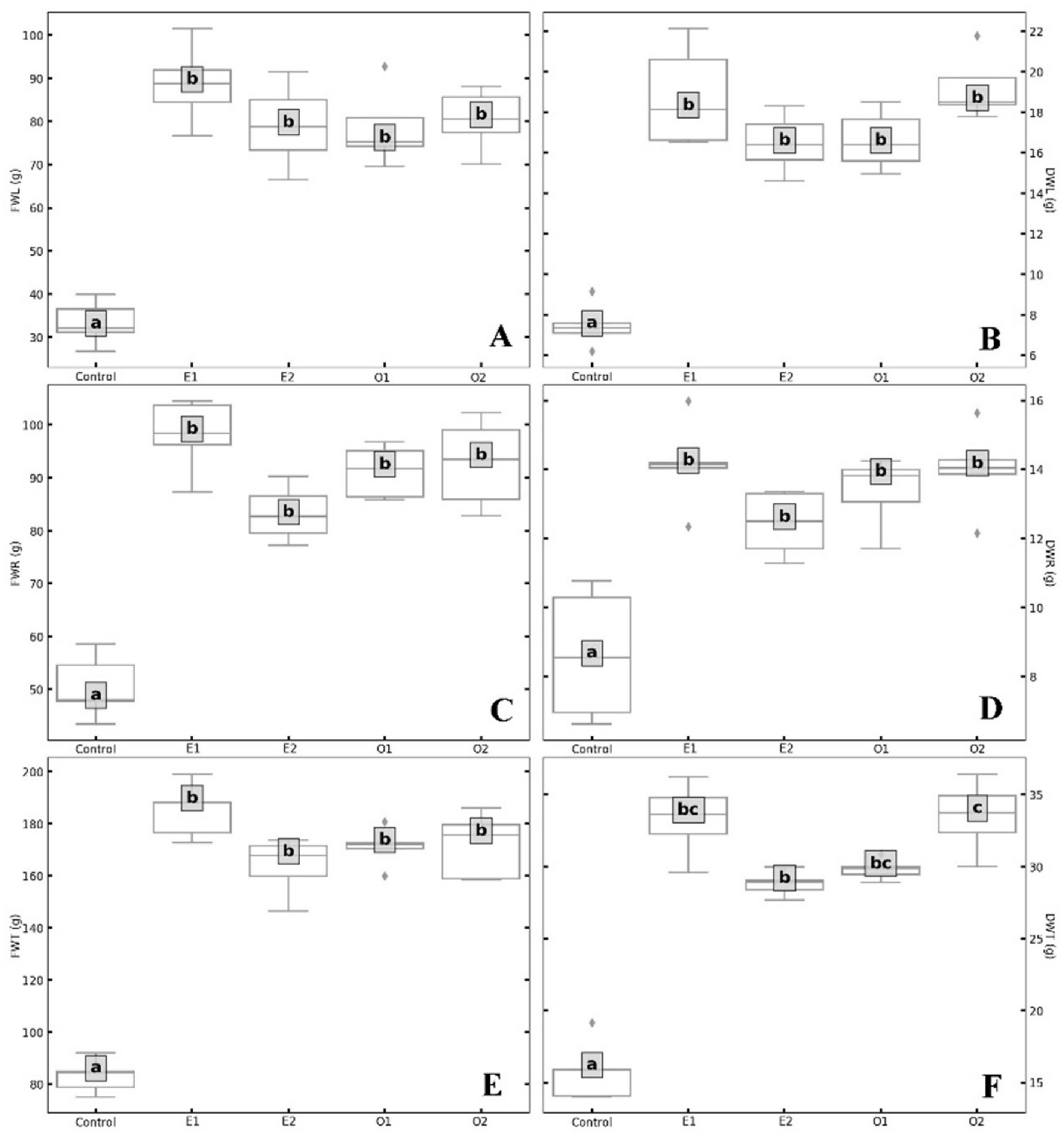
Table A3). Analysis of the different growth parameters showed statistically significant differences. The treated plants showed an average fresh leaves weight (81.6 g) that was about 48 g greater than the Control plants; and the higher value of FWL was observed in the E1 treatment with 88.7 g (Figure 1A; Table A4). Leaves dry weight (DWL) showed an increase from 120% (O1; E2) to about 150% (O2; E1) compared to the Control (Figure 1B and Table A4). The highest values of DWL were observed in E1 and O2, with 18.8 and 19.2 g respectively. Leaves fresh and dry weights showed no statistically significant differences among treatments with the two biostimulants (Figure 1A,B, Table A4).
Regarding the grown factors FWL and DWL, the pairwise analysis (Table A2) showed that the practical significance, expressed in terms of Effect Size is always significant (EF < −5.3) in the comparison between Control and Treatments (E1, E2, O1, O2) and the most significant effects were recorded between Control and O2 (EF = −6.8 for FWL and EF = −7.8 for DWL) (Table A2). Comparing the treatments in pairs, for FWL the higher value of EF was obtained for E1⇔O1 (EF = 1.01), while the minimum difference of response was obtained by comparing the groups E2⇔O1 (EF = 0.046). DWL showed a higher value of EF when comparing in pair E2⇔O2 (EF = −1.64), and the minimum difference in E2⇔O1 (EF = −0.094) (Table A2). Concerning roots fresh and dry weights, they were significantly higher in EM and OMW treatments compared to the Control (Figure 1C,D; Table A4). The increase in fresh weight ranged from 65% (E2) to 94.4% (E1), and the highest value of FW roots was recorded in the E1 treatment with 98.0 g (Figure 1C; Table A4). For the dry weight, the best values were observed in E1 (14.1 g) and O2 (14.0 g) treatments, while the Control recorded 8.6 g (Figure 1D). Roots fresh and dry weights showed no statistically significant differences between treatments with the two biostimulants (Figure 1C,D). Comparing the Control with the treatments the pairwise analysis (Table A2) showed that the maximum response to treatment for FWR was observed for pair Control⇔O1 (EF = −6.67), while among the treatments the maximum value of EF was observed for pair E1⇔E2 (2.17). Instead for DWR, the comparison between Control and treatments exhibited the maximum value for pair Control⇔E1 (EF = −3.08) and the minimum difference in Control⇔E2 (EF = −2.30). In treated plants maximum differences were observed for pair E1⇔E2 and the minimum in E1⇔O2, EF = 1.38 and EF = 0.10 respectively (Table A2). The total fresh (FWT) and total dry weight (DWT) of OMW- and EM-treated plants were always higher in all treatments compared to Control. The treated plants showed an average FWT (172.9 g) that was about 89 g greater than the Control plants, and a higher value was observed in E1 (184.9 g) (Table A4). The highest value in the pairwise analysis was EF = 11.4 in Control⇔O1 (Table A2). The FWT did not show statistically significant differences among the four treatments (Figure 1E). Regarding DWT, the treatments E1 and O2 registered the highest mean values (33.3 g and 33.5 g, respectively) and marginally significant differences were observed between the two biostimulants and the applied concentrations (Figure 1F; Table A4). Control in comparison to treated plants, showed the maximum value of EF (−8.07) for pair Control⇔O1, among treatments the minimum was for E1⇔O2 (EF = −0.06), and the highest was for E2⇔O2 (EF = −2.29) (Table A2). The improved development of treated plants with EM and OMW is highlighted also in an increase in the total RGR index (Figure 2).
At the end of the experiment (75 DTA), the total RGR of treated plants ranged from 50.5 to 53.1 mg g 1 d 1 , with the highest value in O2 treatment, while in the Control was 40.3 mg g 1 d 1 . In all plants the aerial part (leaves) exhibited the highest RGR and, in particular, the treated plants showed a significant increase of about 32% in leaves RGR compared to the Control; the highest value was observed in OMW treatment applied at the maximum concentration (O2; 63.0 mg g 1 d 1 ).
The increased growth observed in Tanacetum balsamita treated plants, can be attributed to the biostimulants influence and the effect is evident in both the rooting system and the aerial biomass development. In literature, several studies reported on horticultural and ornamental plants, the positive influence of microorganism activity (EM) on plant growth parameters [36,37,38,39]. In Figure 3 the plants at T0 and T3 are shown, with details of leaves and roots.
The positive application of EM and OMW resulted also, in an increases in values of leaves number (LN) and leaf area (LA) (Table A4; Figure 3 and Figure 4A,B). The average number of leaves in plants treated with OMW and EM (181.6) enhanced by 78.5% with respect to the Control; the highest values were observed applying the minor biostimulant concentrations, O1 (205 leaves) and in E1 (185.8 leaves) (Figure 4A; Table A4). Control plants registered a mean leaf area of 39.1 cm 2 while treatments determined an increase of leaf area ranging from about 72.0 cm 2 in E1 to 42.1 cm 2 in O1 (Figure 4B; Table A4).
Comparing the Control with the treatments the pairwise analysis (Table A3) showed that the maximum value of EF for LN was −8.03 (Control⇔O1) and the minimum was −5.95 for Control⇔E2, however, the latter value highlights a strong response to treatment. Among the treatments, the maximum value was observed for E2⇔O1 (EF = −3.54) and the minimum was for E1⇔O2 with EF = 0.99 (Table A3). Instead for LA, the comparison between Control and treatment exhibited the maximum value in Control⇔E1 (EF = −4.4) and the minimum difference in Control⇔O1 (EF = −0.51) (Table A3). In treatment plants, maximum differences were observed in E1⇔O1 and the minimum in E1⇔O2, EF = 3.84, and EF = 0.69 respectively (Table A3). Regarding these results, O1 treatment recorded a leaf area value similar to the Control, but the best result was in leaves number (205). This result is not conflicting, Hassanpouraghdam et al. [14] had already observed an inverse relationship between leaf area and leaf number in Tanacetum balsamita plants treated with different concentrations of N, and they considered this result to be not limiting to plant growth. The estimation of leaf number and leaf area is decisive for plant growth and development being the leaf an essential plant structure that allows gas exchange and the transformation of light energy into chemical energy useful for cellular functions [40]. The effects of EM and OMW treatments on growth indices SLA (Specific Leaf Area), LAR (Leaf Area Ratio), and LWR (Leaf Weight Ratio), are reported in Table A1 and Figure 4C–E. SLA is a measure of leaf thickness, correlated with the number and/or size of leaf photosynthetic mesophyll cells [41]. SLA index showed similar values for E2, O1, and O2 treatments and Control, while E1 treatment reported the highest value (715.2 cm 2 g 1 ; Figure 4C). LWR describes the efficiency of assimilation in the whole plant. LWR index ranged from 0.59 in O2 to 0.47 g g 1 in the Control and did not show differences between treated plants, which however showed values higher than the Control (Table A4; Figure 4D). LAR defines the leaf area produced per unit of biomass and therefore it is closely related to photosynthetic activity. In the present study LAR index values in treated plants were higher compared with the Control, and the highest data was recorded in E1 (414.9 cm 2 g 1 ) followed by O2 treatment with 353.1 cm 2 g 1 (Table A4; Figure 4E). Comparing the Control with the treatments the pairwise analysis (Table A3) showed that the maximum value of EF for SLA was −1.31 (Control⇔E1) and the minimum was 0.03 for Control⇔O1. Among the treatments, the maximum value was observed for E1⇔E2 (EF = 2.11) and the minimum was EF = −0.05 for E2⇔O1 (Table A3). Instead for LWR, the comparison between Control and treatment exhibited the maximum value in Control⇔O2 (EF = −3.54) and the minimum difference in Control⇔O1 (EF = −2.20) (Table A3). LAR showed among Control and treatment the maximum value of EF = −2.62 in Control⇔E1 and the minimum in Control⇔O1 (EF = −0.74). The highest value among treated plants was EF = 2.37 in E1⇔E2, and the lowest was in E2 ⇔O1 with EF = 0.27 (Table A3).
In our experimental conditions, EM and OMW determined an increase in leaf number and leaf area but did not affect leaf thickness. These results agree with Scavroni et al. [42] that used organic fertilizers in Mentha piperita L. and with Wadas and Dziugieł [43] for the use of biostimulants in Solanum tuberosum L. The rise of LWR and LAR, due to the application of biostimulants, in combination with enlarged leaf size, can maximize the optical light interception efficiency and the greater acquisition of resources resulting in an increment of plant growth [44,45,46].
The presence of trichomes on the leaf surface of Tanacetum balsamita was observed, and thus effect of biostimulants on the number of trichomes was evaluated. Although trichomes have been described in some species of the genus Tanacetum, this is the first time they are described in Tanacetum balsamita. Costmary presented non-glandular and glandular trichomes on the adaxial and abaxial epidermis (Figure 5A–F), even if they are both more abundant on the lower epidermis. Non-glandular trichomes are long, uniseriate T-shaped hair and consist of 2–3-foot cells and 2 acicular armed hair (Figure 5A,B,G). Glandular trichomes consist of biseriate secretory cells and a large subcuticular cavity where secretory products are stored, like the peltate trichomes of the Lamiaceae ([47,48] (Figure 5C–E,G). Histochemical staining (Nadi Reagent) and fluorescence analysis highlighted the presence of terpenes and wall-bound hydroxycinnamates in glandular trichomes (Figure 5D,E) [49,50]. Under our experimental conditions, no statistically significant difference among treatments was found in the density of glandular trichomes while in non-glandular trichomes, the number was significantly higher in the E2 (81.3) and O1 (78.7) treatments compared to the Control (64.7) (Figure 5F–L). These results agree with the study of Saour [51] who reported an increase in non-glandular hairs in potato plants after treatments with commercial organic biostimulant (Vitazyme™) speculating a positive relationship among the action of biostimulant, the resistance to pathogens and trichomes number.
Until now, there is no published research on the use of EM and OMW in costmary. Many studies reported a positive effect of EM on a wide range of fruits and leafy vegetables in pot and in field experiments [52], such as apples [53], beans [54] and tomato [55]. Similarly pot experiments under greenhouse, reported in Allium cepa [21] an increase in bulb growth parameters and in the medicinal plants Bulbine frutescens [22], a significant improvement in the number of new leaves, shoots, inflorescences per plant, and biomass weight. The efficiency of EM is attributed to the increase in the photosynthesis, in microbial biomass and to the improvement of water supply. EM also stimulates plant growth by improving physiological processes and plant resistance to abiotic stresses producing bioactive substances such as hormones and enzymes, accelerating the decomposition of organic materials, and controlling soil diseases [56,57,58,59]. Although most published studies show a positive effect of EM on plant growth, some researches reported negative or non-significant effects [52], as well as in sweet corn [60], seeds cotton [61] and Chinese cabbage [62]. Few information on the application of OMW on plants is available. OMW has a high content of organic compounds, and macro and microelements, making it valuable as biofertilizers and/or biostimulants. However, OMW obtained during oil production has a high level of acidity, salinity, and polyphenol content that make it harmful [63]. Indeed, the application of undiluted OMW resulted in the suppression of seeds germination in Triticum durum L. [64], Vicia faba L. and Cicer arietinum L. [65]. In addition, it was reported that the use of the unmodified OMW has a negative impact on physico-chemical and biological soil properties and ground waters [65]. To make this product usable in agriculture, it is necessary to remove the detrimental products. Several methods have been developed for the improvement of OMW and the resulting product has been evaluated in different plants [66]. In our experimental study, to reduce toxicity, OMWs were treated by a simple and easily repeatable method: decantation, dilution, and pH adjustment. Our findings are in agreement with [23], where the filtered OMW applied to tomato plants increased growth parameters and fruit size. Other researchers have observed the same results in Triticum aestivum var. Douma1 [61], in Vicia faba L. and Cicer arietinum L. [65], and Phaseolus vulgaris L. [67]. The positive effects of OMWs application are attributed to the large quantity of protein, polysaccharides, humic acids, and macro and micro mineral elements present in this compound [23].

3.2. Mineral Composition of Leaves

The results of the mineral analysis, as tissue concentration, performed on costmary plants at 0 DAT (T0) and 75 DAT (T3) in Control, E1, E2, O1, O2, are shown in Figure 6. The development of root, shoot, and leaves allowed more functional nutrient assimilation, and transport of mineral elements and physiological activators, as already seen by De Pascale et al. [68].
After 75 DAT (T3), Control plants had a typical enhancement of the nutrient content (Figure 6). The mineral element concentrations were differently affected by the type of treatment and treatment concentration. Total N showed the highest values in plants grown on E2 and O2 (28.79 ± 0.34 g Kg 1 DW and 30.23 ± 0.65 g Kg 1 DW, respectively), the highest concentrations used in this experiment. On the other hand, in these plants, N-NO3 was significantly lower (0.93 ± 0.03 g Kg 1 DW and 0.82 ± 0.04 g Kg 1 DW, for E2 and O2, respectively) respect to the Control at T3 and the treated plants with the lowest concentrations (E1 and O1) indicating that these treatments could be useful to reduce nitrates in this edible plant. In fact, an excess consumption of nitrates is considered dangerous because nitrates could be converted into nitrite in the gut and nitrite can bind to hemoglobin preventing the blood from carrying enough oxygen or, in presence of ammine, may generate nitrosamines, known to have carcinogenic activity [69]. For this reason, the reduction of anti-nutritional factors in horticultural products, such as nitrates in leafy vegetables, has become an important objective in agricultural research. Phosphate concentrations in plants treated with the highest concentrations of EM and OWM (E2, 1.10 ± 0.09 g Kg 1 DW; O2, 0.99 ± 0.22 g Kg 1 DW) were significantly minor to those of Control at T3 (2.13 ± 0.04 g Kg 1 DW), E1 (2.91 ± 0.10 g Kg 1 DW), and O1 (2.09 ± 0.23 g Kg 1 DW). Accordingly, K contents decreased significantly with the high EM and OMW concentrations (Control, 1.73 ± 0.01 g Kg 1 DW; E1, 2.01 ± 0.01 g Kg 1 DW; E2, 0.47 ± 0.03 g Kg 1 DW; O1, 2.19 ± 0.05 g Kg 1 DW; O2, 0.23 ± 0.02 g Kg 1 DW). A significant increase in sodium and magnesium was observed adding EM and OMW at the substrates compared with Control (Na, 0.13 ± 0.01 g Kg 1 DW; Mg, 1.03 ± 0.01 g Kg 1 DW), the application of biostimulant compounds seem to increase the availability of these mineral elements for the plant. Calcium was the only element affected simultaneously both by treatment and by the treatment concentrations. Specifically, it was higher in Control (11.60 ± 0.40 g Kg 1 DW). The other elements were all influenced by treatment and concentration.
The EM application has also been investigated in tomatoes [70], and grass species [71]. The authors showed that the addition of EM may enhance the amount of some elements, such as nitrogen, phosphorus, and potassium, promoting growth and productivity. These findings support the results of E1 and E2 treated plants which exhibited also higher growing parameter values with respect to the Control plants.

3.3. Physiological Parameters: Chlorophyll a Fluorescence

The trend of the JIP-test parameters is reported in Figure 7. The values measured for the following parameters F v F m ; Mo; VJ; ϕ Eo, in all the plants at T0 did not exhibit significant differences. These parameters are a useful tool to measure the electron transfer efficiency between the two photosystems of the photosynthetic apparatus, and their variations indicate how the level of this efficiency decreases, in the presence of stress. The F v F m parameter is a measure of the maximum quantum yield of PSII for primary photochemistry, and a lowering of this value reflects a decrease in the ability to carry out photosynthesis. As shown in Figure 7A the photosynthetic activity, expressed as F v F m did not exhibit large variations during the period of the experiment (T0–T3). During the period of the treatment, at each time, no significant changes were detected among the Control and the treated plants, indicating that all the treated plants maintained efficient photosynthetic activity. However, it is interesting to underline that all the treated plants showed F v F m values higher than Control plants, at any time, till T3. The highest values at T3 were detected in O1 and E1 (8.5% and 6.3%). The changes of the parameter Mo are reported in Figure 7B. This parameter is a measure of the efficiency of the reaction centers to transfer electrons into the electron transport chain, and it increases when this efficiency is reduced. The results showed that, during the period of the treatments (T0–T3), all the treated plants exhibited a declined value of Mo. At T3 the highest changes resulted for E1, O1, and O2, whereas only a slight decline, by 2.10% and 4.41%, could be observed for E2 and Control, respectively Figure 7B. Anyway, changes in this parameter indicated better performance of the reaction centers tendentially in the treated plants.
Figure 7C shows the changes in the VJ parameter. The VJ value reflects the reduction state of the photosynthetic apparatus, at the plastoquinone level, and it is a very useful tool to follow the level of accumulation of electrons in the electrons transport chain during the growth and especially under stress conditions which may affect the photosynthetic activity [72]. The value of this parameter, during the examined period, from T0 to T3, resulted unchanged in E2 while it decreased in the other treated plants (O1, E1 and O2) (Figure 7C), a significant change was observed only for O2. At T3 the differences among the VJ values were not significant among the plants. Anyway, the lowering of this parameter, indicated that, during the growth, both OMW and EM exercised a positive effect on photosynthetic electrons transport efficiency. The changes of the parameters ϕ Eo are reported in Figure 7D. The results indicated that it tendentially improved in all the plants at T3, except E2. The highest increase was observed in the following order: O2, O1, E1, and Control (23.87%, 16.90%, 15.22%, and 2.48% respectively). Comparison of the values at T3 showed significant differences for O1 vs. E2, O2 vs. E2, and E1 vs. E2. Also, for this parameter, the results tendentially showed a better performance in the treated plants. The implementation, although slight, of the photosynthetic efficiency in the treated plant with OMW and EM agrees with plant growth parameters, in particular the leaves number and leaf area (Figure 1). The fluorescence parameters measurements showed that the addition of OMW to the plants was not toxic, at the assessed concentration.
The slight improvement of the photosynthetic efficiency in the treated plant with EM and OMW is in agreement with plant growth parameters, in particular the leaves number and leaf area (Figure 1). The fluorescence indices measurement showed that the addition of OMW to the plants was not toxic, at the assessed concentrations. These results confirmed previous findings, reporting that the application of diluted filtered OMW, at neutral pH, incremented both growth and photosynthetic efficiency in tomato plants [23] and in olive trees [72]. The authors reported the increment of chlorophyll fluorescence parameters in olive trees (Olea europaea L. cv. Chemlalì) when soil tillage was combined with OMW irrigation, they associated these results with the attenuation of oxidative stresses [72]. Our findings agree with these results, as O1 and O2 treatments enhanced the photosynthetic activity, electron transport efficiency, and attenuation of reductive conditions at the photosynthetic apparatus level. Several protocols are used for the management of OMWs, in order to make them suitable for agriculture application, including mechanical steps of filtration and microbiological treatments [23,73]. In our study, the OMW treatment was very simple, very low time consuming and economically advantageous, as OMW was just kept settling for a week, the pH was adjusted to neutral value, and the right dilution rates were adopted. With this strategy, the toxicity due to the presence of polyphenolic compounds, conferring dark color and very low pH, was strongly reduced. Moreover, this procedure could not alter the organic and chemical composition of the OMW, which may have supplied nitrogen, phosphorus, and potassium [74] with a positive effect of photosynthetic efficiency. The addition of EM may enhance the amount of absorbable nutrients, such as nitrogen, phosphorus, and potassium [71], and maintain a high efficiency of PSII; these are two important processes for plant growth and productivity [54]. These findings support the observed trend in E1 and E2 treated plants which exhibited a facilitated photosynthetic performance.

3.4. Total Polyphenolic Content and Individual Phenolic Determination

The values of the total phenolic content, measured on all the plants at T0, did not exhibit significant differences. In general, the extracts, of both the Control and treated plants, exhibited some changes in the total polyphenolic content during the period of the experiment (T0–T3) (Table 2).
The highest total polyphenolic content significant increase was observed at T1 in the Control and O1 plants, resulting in 29% higher than at the initial time, under both conditions (Table 2). For the other treatments, changes were not relevant, whereas the highest increment was observed after T2, by 7.5%, 18.0% and 19.1%, for O2, O1 and E1 extracts, respectively, while E2 did not induce any polyphenolic increase, with respect to the initial time. At the end of the growth period T3, in the Control and all the treated plants, the differences among the polyphenolic content in the extracts were not significant and the values were in the range of 18.6–20.9 mg g 1 . The individual phenolic composition was quantified, and it is reported in detail in Table 3. Also in this case, the values measured on all the plants at T0 did not exhibit significant differences, for all the phenolic acids. At the initial time caffeic acid, isochlorogenic acid, rutin, and a very small amount of chlorogenic acid were found. As shown in Table 3, these compounds resulted increased tendentially in all the treated plants, at the harvesting time. At T3 the extracts of the treated plants showed a significant higher amount of the phenolic compounds detected, with respect to the Control. For the chlorogenic acid, at a very low concentration at the initial time, the highest content followed the order: O2, E1, E2, O1, in the range of 2.16–2.45-fold higher than Control (Table 3). The same trend could be observed for the caffeic acid, although the differences were less pronounced, in the range of 1.91-fold and 2.11-fold higher than Control. Whereas the amount of caffeic acid was almost the same in all the treatments, by contrast, isochlorogenic acid content showed significant differences among all the plants, except for E1 and Control, ranging from 1.02 to 2.44-fold the amount of Control. Rutin content in the extracts of the treated plants ranged in a value 1.28–1.50-fold the one of the Control extract (Table 3). The phenolic composition resulted interestingly different among the plants. The higher amount of chlorogenic acid, caffeic acid, isochlorogenic acid, and rutin with respect to the Control plants evidenced how the improvement of the photosynthesis in these plants promoted a positive effect on the production of these antioxidant compounds.The value of total polyphenolic content may result non proportional to or higher than the value obtained by adding all the phenolic compounds quantified by HPLC analyses, and this is our case. The explanation is that the method to determine the total phenolic content may imply the reaction of a hydroxyl group of all phenolic compounds and their degradation product, which cannot be detected by HPLC analysis [75].
It is generally reported that the increment of polyphenolic substances, such as other antioxidants, is induced by the occurrence of oxidative stresses, to counteract the effect of the presence of free radicals [76,77]. However, many officinal plants, such as Tanacetum balsamita L., are constitutively able to produce a high amount of polyphenols also in absence of oxidative stress [13,19]. In the present study, stress in plants did not occur, neither in Control nor in treated plants, as revealed by fluorescence measurements. The most relevant result concerned the presence of important antioxidant phenolic compounds, in all the treated plants, at a concentration higher than in the Control ones and these results underline the importance of the utilization of both OMW and EM. The phenolic acids found in the extracts are well-known compounds synthesized in costmary, which can confer to the leaves anti-inflammatory, carminative and detoxifying properties [19,78].

3.5. Antiradical Activity

Changes in the values of the antiradical activity are reported in Table 3. At the initial time, the I50 value was 0.43 ± 0.01. At T3 the increment of the antiradical activity could be observed particularly in O2 and E2, that showed high level of chlorogenic, isochlorogenic and caffeic acids. Only Control and E1 extracts did not show significant differences with the values of T0. Interestingly, the most consistent I50 decrease was shown by the extracts of the plants treated with the highest concentration, E2 and O2 (42% and 39%, respectively), followed by O1 and E1 (26% and 12%, respectively) (Table 3). In the Control plants, I50 decreased only by 7.5%. The highest antiradical activity showed in all the treated plants fitted with the highest concentration of phenolic compounds in their extracts, which may act as antioxidants [19,79,80], particularly in O2 and E2, that recorded high level of chlorogenic, isochlorogenic and caffeic acids. In this regard, considering that the total polyphenolic content was not significantly different among all the extracts, the qualitative phenolic composition influenced the antioxidant properties of the extracts.

3.6. Principal Component Analysis (PCA)

PCA does not discard any samples or characteristics (variables) but it reduces the overwhelming number of dimensions by constructing principal components (PCs) that describe the variation of the original characteristics. Such influences, or loadings, can be traced back from the PCA plot to find out what produces the differences among clusters. Thus, Principal Component Analysis was performed to obtain a smaller number of linear combinations of all considered variables which were significantly representative of the experimental results (see Section 2.8—Statistical analysis). Three main components were extracted that had eigenvalues greater than 1.0. Together they accounted for 85.1% of the variability in the original data (Table 4). The first and second components of the PCA accounted for 50.0% and 24.6% respectively of the total variation of the traits investigated (Table 4).
The eigenvectors divided satisfactorily the concentrations of the treatments but not the different treatments. There were three groups into three main sectors of the score plot of which Control and low concentrations were separated from the highest ones by the principal component (Figure 8A). Nitrate, K, phosphate, Ca and total polyphenols were positively correlated (at the highest level) with the first principal component. The opposite was observed for N and Mg amounts. The number of leaves was positively correlated with the second principal component. Instead, Na concentrations in plant tissues were positively correlated (at the highest level) with the third principal component, while the opposite tendency was observed for the total plant dry biomass (total DWT). However, photosynthesis showed a high correlation with the second component (Figure 8B, Table 4). The nutrient content of the plants mostly explained the variability in the dataset (Figure 8B). Figure 8 showed a broad separation of the treatments concentration due to significant variations in nutrient levels. The results emphasize how the patterns of covariance found are similar in the two treatments and it is mainly due to the concentration rather than the type of biostimulant.

4. Conclusions

The results of the present study showed that Effective Microorganisms and Olive Mill Wastewater application can effectively improve the growth and physiology performance of Tanacetum balsamita L. in relation to the concentrations used. More specifically, the experiment showed that the two biostimulants applied to the substrate, had positive effects, with statistically significant differences, on fresh and dry weight and plant growth respect to the Control. In addition, all the treated plants maintained efficient photosynthetic activity, reporting, at the end of the experiment, a higher F v F m than the Control. Finally, EM and OMW improved the concentration of the phenolic compounds and antiradical activity of costmary plant. This study confirms the effectiveness of EM to increase the growth and quality of plants and in particular, points out the potential use of OMW on cultivated crops. There are few studies analyzing OMW as a biostimulant and our results demonstrate that this waste product, at the used concentrations, improved costmary plant performance without negative effects on the quality and quantity of secondary metabolites. Further studies are necessary to better define the standardization of the use of OMW, optimizing concentrations and methods of administration to different plants, and safeguarding the environment.

Author Contributions

Conceptualization, C.F., C.G., C.B. and R.P.; methodology, C.F., C.G., C.B., S.D.L., L.A. and R.P.; validation: C.F., C.G., C.B., S.D.L., L.A. and R.P.; formal analysis: C.F., C.G., C.B., S.D.L., R.P., M.A. and F.S.; investigation: C.F., C.G., C.B., S.D.L., L.A. and R.P.; data curation: C.F., C.G., C.B., S.D.L., L.A. and R.P.; writing-original draft preparation: C.F., C.G., C.B., S.D.L., L.A. and R.P.; writing-review and editing: C.F., C.G., C.B., S.D.L., L.A. and R.P.; supervision: C.F., C.G., C.B., S.D.L., L.A. and R.P.; All authors have read and agreed to the published version of the manuscript.

Funding

This research received no external funding.

Institutional Review Board Statement

Not applicable.

Informed Consent Statement

Not applicable.

Data Availability Statement

Not applicable.

Conflicts of Interest

The authors declare no conflict of interest.

Appendix A

Table A1. Chemical composition of Olive Mill Wastewater (OMW) used for costmary treatment.
OMW Composition
Total polyphenols (gL 1 )3.87 ± 0.27
Phosphates (mgL 1 )668.00 ± 34.42
Sulphates (mgL 1 )61.50 ± 14.85
Nitrates (mgL 1 )8.67 ± 0.48
Cu (mgL 1 )3.97 ± 1.28
Mg (mgL 1 )203 ± 32.53
K (mgL 1 )11.9 ± 2.93
Ca (mgL 1 )604.00 ± 32.22
Carbohydrates (gL 1 )8.26 ± 1.52
Proteins (gL 1 )9.68 ± 1.98
Ashes (%)0.75 ± 0.04
COD (gO2L 1 )52.25 ± 0.56
BOD516.05 ± 0.31
Table A2. Treatments pairwise analysis for growth factors.
Growing f.ABmean (A)std (A)mean (B)std (B)Tdofp-uncp-corrp-adjustEffect Size
DWL (g)ControlO27.481.0719.231.58−13.7180.000.00bonf−7.83
DWL (g)ControlO17.481.0716.621.47−11.2580.000.00bonf−6.43
DWL (g)ControlEM27.481.0716.471.45−11.1580.000.00bonf−6.37
DWL (g)ControlEM17.481.0718.802.49−9.3380.000.00bonf−5.33
DWL (g)EM2O216.471.4519.231.58−2.8780.020.21bonf−1.64
DWL (g)O1O216.621.4719.231.58−2.7080.030.27bonf−1.54
DWL (g)EM1EM218.802.4916.471.451.8180.111.00bonf1.03
DWL (g)EM1O118.802.4916.621.471.6980.131.00bonf0.96
DWL (g)EM1O218.802.4919.231.58−0.3280.761.00bonf−0.18
DWL (g)EM2O116.471.4516.621.47−0.1780.871.00bonf−0.09
DWR (g)ControlEM18.641.8914.141.28−5.3980.000.01bonf−3.08
DWR (g)ControlO28.641.8914.001.25−5.3080.000.01bonf−3.03
DWR (g)ControlO18.641.8913.371.03−4.9280.000.01bonf−2.81
DWR (g)ControlEM28.641.8912.430.93−4.0380.000.04bonf−2.30
DWR (g)EM1EM214.141.2812.430.932.4180.040.42bonf1.38
DWR (g)EM2O212.430.9314.001.25−2.2580.050.54bonf−1.29
DWR (g)EM2O112.430.9313.371.03−1.5180.171.00bonf−0.86
DWR (g)EM1O114.141.2813.371.031.0580.321.00bonf0.60
DWR (g)O1O213.371.0314.001.25−0.8880.411.00bonf−0.50
DWR (g)EM1O214.141.2814.001.250.1880.861.00bonf0.10
DWT (g)ControlO115.802.0929.820.74−14.1380.000.00bonf−8.07
DWT (g)ControlEM215.802.0928.800.85−12.8780.000.00bonf−7.35
DWT (g)ControlO215.802.0933.492.46−12.2480.000.00bonf−6.99
DWT (g)ControlEM115.802.0933.312.53−11.9180.000.00bonf−6.80
DWT (g)EM2O228.800.8533.492.46−4.0280.000.04bonf−2.30
DWT (g)EM1EM233.312.5328.800.853.7780.010.06bonf2.15
DWT (g)O1O229.820.7433.492.46−3.1980.010.13bonf−1.82
DWT (g)EM1O133.312.5329.820.742.9580.020.18bonf1.69
DWT (g)EM2O128.800.8529.820.74−2.0480.080.76bonf−1.16
DWT (g)EM1O233.312.5333.492.46−0.1280.911.00bonf−0.07
FWL (g)ControlO233.275.0980.407.10−12.0680.000.00bonf−6.89
FWL (g)ControlEM133.275.0988.689.19−11.7980.000.00bonf−6.74
FWL (g)ControlO133.275.0978.558.89−9.8880.000.00bonf−5.65
FWL (g)ControlEM233.275.0979.039.77−9.2980.000.00bonf−5.31
FWL (g)EM1O188.689.1978.558.891.7780.121.00bonf1.01
FWL (g)EM1EM288.689.1979.039.771.6180.151.00bonf0.92
FWL (g)EM1O288.689.1980.407.101.5980.151.00bonf0.91
FWL (g)O1O278.558.8980.407.10−0.3680.731.00bonf−0.21
FWL (g)EM2O279.039.7780.407.10−0.2580.811.00bonf−0.14
FWL (g)EM2O179.039.7778.558.890.0880.941.00bonf0.05
FWR (g)ControlO150.436.0191.174.97−11.6880.000.00bonf−6.67
FWR (g)ControlEM150.436.0198.046.91−11.6280.000.00bonf−6.64
FWR (g)ControlO250.436.0192.718.34−9.1980.000.00bonf−5.25
FWR (g)ControlEM250.436.0183.245.26−9.1880.000.00bonf−5.25
FWR (g)EM1EM298.046.9183.245.263.8180.010.05bonf2.18
FWR (g)EM2O183.245.2691.174.97−2.4580.040.40bonf−1.40
FWR (g)EM2O283.245.2692.718.34−2.1580.060.64bonf−1.23
FWR (g)EM1O198.046.9191.174.971.8080.111.00bonf1.03
FWR (g)EM1O298.046.9192.718.341.1080.301.00bonf0.63
FWR (g)O1O291.174.9792.718.34−0.3580.731.00bonf−0.20
FWT (g)ControlO183.096.47171.157.42−20.0080.000.00bonf−11.43
FWT (g)ControlEM183.096.47184.9410.47−18.5080.000.00bonf−10.57
FWT (g)ControlEM283.096.47163.8811.06−14.1080.000.00bonf−8.05
FWT (g)ControlO283.096.47171.7012.53−14.0580.000.00bonf−8.03
FWT (g)EM1EM2184.9410.47163.8811.063.0980.010.15bonf1.77
FWT (g)EM1O1184.9410.47171.157.422.4080.040.43bonf1.37
FWT (g)EM1O2184.9410.47171.7012.531.8180.111.00bonf1.04
FWT (g)EM2O1163.8811.06171.157.42−1.2280.261.00bonf−0.70
FWT (g)EM2O2163.8811.06171.7012.53−1.0580.331.00bonf−0.60
FWT (g)O1O2171.157.42171.7012.53−0.0880.941.00bonf−0.05
Table A3. Treatments pairwise analysis for leaves.
Leaf FeaturesABmean (A)std (A)mean (B)std (B)Tdofp-uncp-corrp-adjustEffect Size
LA (cm 2 )ControlEM139.126.0672.059.40−11.04160.000.00bonf−4.40
LA (cm 2 )ControlO239.126.0666.257.28−12.82330.000.00bonf−4.03
LA (cm 2 )EM1O172.059.4042.134.989.74220.000.00bonf3.84
LA (cm 2 )O1O242.134.9866.257.28−10.78280.000.00bonf−3.62
LA (cm 2 )ControlEM239.126.0656.127.01−7.17190.000.00bonf−2.60
LA (cm 2 )EM2O156.127.0142.134.985.63220.000.00bonf2.22
LA (cm 2 )EM1EM272.059.4056.127.014.71220.000.00bonf1.85
LA (cm 2 )EM2O256.127.0166.257.28−3.82240.000.01bonf−1.37
LA (cm 2 )EM1O272.059.4066.257.281.81200.090.86bonf0.69
LA (cm 2 )ControlO139.126.0642.134.98−1.59260.121.00bonf−0.51
LARControlEM1256.0758.64414.9461.03−7.51210.000.00bonf−2.62
LAREM1EM2414.9461.03308.1527.215.70140.000.00bonf2.38
LAREM1O1414.9461.03298.0647.155.25220.000.00bonf2.07
LARControlO2256.0758.64353.1352.44−5.70390.000.00bonf−1.70
LAREM1O2414.9461.03353.1352.442.87210.010.09bonf1.07
LARO1O2298.0647.15353.1352.44−3.00250.010.06bonf−1.06
LARControlEM2256.0758.64308.1527.21−3.90360.000.00bonf−1.06
LAREM2O2308.1527.21353.1352.44−3.23340.000.03bonf−1.05
LARControlO1256.0758.64298.0647.15−2.34270.030.27bonf−0.74
LAREM2O1308.1527.21298.0647.150.67160.511.00bonf0.27
LN nControlO1101.729.34205.0013.52−14.0580.000.00bonf−8.03
LN nControlO2101.729.34175.048.17−13.2280.000.00bonf−7.55
LN nControlEM1101.729.34185.7611.17−12.9180.000.00bonf−7.37
LN nControlEM2101.729.34160.688.53−10.4280.000.00bonf−5.96
LN nEM2O1160.688.53205.0013.52−6.2080.000.00bonf−3.54
LN nO1O2205.0013.52175.048.174.2480.000.03bonf2.42
LN nEM1EM2185.7611.17160.688.533.9980.000.04bonf2.28
LN nEM2O2160.688.53175.048.17−2.7280.030.26bonf−1.55
LN nEM1O1185.7611.17205.0013.52−2.4580.040.40bonf−1.40
LN nEM1O2185.7611.17175.048.171.7380.121.00bonf0.99
LWRControlO20.470.030.590.03−11.72370.000.00bonf−3.54
LWRControlEM20.470.030.570.03−10.24380.000.00bonf−3.08
LWRControlEM10.470.030.570.05−6.96160.000.00bonf−2.72
LWRControlO10.470.030.560.05−5.61160.000.00bonf−2.21
LWRO1O20.560.050.590.03−1.91170.070.72bonf−0.75
LWREM2O20.570.030.590.03−1.54340.131.00bonf−0.50
LWREM1O10.570.050.560.050.96220.351.00bonf0.38
LWREM2O10.570.030.560.050.90170.381.00bonf0.35
LWREM1O20.570.050.590.03−0.75180.461.00bonf−0.29
LWREM1EM20.570.050.570.030.29170.771.00bonf0.12
SLAEM1EM2715.2297.44541.8166.005.39180.000.00bonf2.11
SLAEM1O1715.2297.44545.6696.084.29220.000.00bonf1.69
SLAControlEM1549.48134.39715.2297.44−4.26290.000.00bonf−1.31
SLAEM1O2715.2297.44607.9472.523.26190.000.04bonf1.25
SLAEM2O2541.8166.00607.9472.52−2.86340.010.07bonf−0.93
SLAO1O2545.6696.08607.9472.52−1.91190.070.71bonf−0.73
SLAControlO2549.48134.39607.9472.52−1.83380.070.74bonf−0.51
SLAControlEM2549.48134.39541.8166.000.25370.811.00bonf0.07
SLAEM2O1541.8166.00545.6696.08−0.12180.911.00bonf−0.05
SLAControlO1549.48134.39545.6696.080.10290.921.00bonf0.03
Table A4. Effect of different applications of biostimulants on the growth parameters of Tanacetum balsamita L. (Means and SE).
ParametersControlE1E2O1O2
LEAVES
FWL (g)33.3 ± 5.188.7 ± 9.279.0 ± 9.878.5 ± 8.980.4 ± 7.1
DWL (g)7.5 ± 1.118.8 ± 5.516.5 ± 1.416.6 ± 1.519.2 ± 1.6
LN (n)101.7 ± 9.3185.8 ± 11.2160.7 ± 8.5205.0 ± 13.5175.0 ± 8.2
LA (cm 2 )39.1 ± 6.172.0 ± 9.456.1 ± 7.042.1 ± 4.966.2 ± 7.3
DWL (%)22.521.220.421.623.9
ROOTS
FWR (g)50.4 ± 6.098.0 ± 6.983.2 ± 5.391.2 ± 4.992.7 ± 8.3
DWR (g)8.64 ± 1.914.1 ± 1.312.4 ± 0.913.4 ± 1.014.0 ± 1.2
DWR (%)17.114.414.914.715.1
TOTAL PLANT
FWT (g)83.1 ± 6.5184.9 ± 10.5163.9 ± 11.1171.1 ± 7.4171.7 ± 12.5
DWT (g)15.8 ± 2.133.3 ± 2.528.8 ± 0.829.8 ± 0.733.5 ± 2.5
DWT (%)19.018.017.617.419.5
GROWTH INDICES
SLA (cm 2 g 1 )549.5 ± 134.4715.2 ± 97.4541.8 ± 66.0545.7 ± 96.1607.9 ± 72.5
LAR (cm 2 g 1 )256.1 ± 58.6414.9 ± 61.0308.1 ± 27.2298.0 ± 47.1353.1 ± 52.4
LWR (g g 1 )0.47 ± 0.030.57 ± 0.050.57 ± 0.030.56 ± 0.050.59 ± 0.03

References

  1. Du Jardin, P. The Science of Plant Biostimulants—A Bibliographic Analysis, Ad Hoc Study Report; European Commission: Brussels, Belgium, 2012. [Google Scholar]
  2. Higashinakagawa, T.; Kikuchi, H.; Kuwayama, H. Mg, K-containing microparticle: A possible active principle of a culture extract produced by a microbial consortium. PLoS ONE 2021, 16, e0259297. [Google Scholar] [CrossRef]
  3. Yousfi, S.; Marín, J.; Parra, L.; Lloret, J.; Mauri, P.V. A Rhizogenic Biostimulant Effect on Soil Fertility and Roots Growth of Turfgrass. Agronomy 2021, 11, 573. [Google Scholar] [CrossRef]
  4. Debska, B.; Kotwica, K.; Banach-Szott, M.; Spychaj-Fabisiak, E.; Tobiašová, E. Soil Fertility Improvement and Carbon Sequestration through Exogenous Organic Matter and Biostimulant Application. Agriculture 2022, 12, 1478. [Google Scholar] [CrossRef]
  5. Ceccon, L.; Saccù, D.; Procida, G.; Cardinali, S. Liquid chromatographic determination of simple phenolic compounds in waste waters from olive oil production plants. J. AOAC Int. 2001, 84, 1739–1744. [Google Scholar] [CrossRef] [Green Version]
  6. Cucci, G.; Lacolla, G.; Caranfa, L. Improvement of soil properties by application of olive oil waste. Agron. Sustain. Dev. 2008, 28, 521–526. [Google Scholar] [CrossRef] [Green Version]
  7. Fountoulakis, M.; Dokianakis, S.; Kornaros, M.; Aggelis, G.; Lyberatos, G. Removal of phenolics in olive mill. wastewaters using the white-rot fungus Pleurotus ostreatus Jacq. Water Res. 2002, 36, 4735–4744. [Google Scholar] [CrossRef]
  8. Paraskeva, P.; Diamadopoulos, E. Technologies for olive mill wastewater (OMW) treatment: A review. J. Chem. Technol. Biotechnol. 2006, 81, 1475–1485. [Google Scholar] [CrossRef]
  9. Lesage-Meessen, L.; Navarro, D.; Maunier, S.; Sigoillot, J.C.; Lorquin, J.; Delattre, M.; Simon, J.L.; Asther, M.; Labat, M. Simple phenolic content in olive oil residues as a function of extraction systems. Food Chem. 2001, 75, 501–507. [Google Scholar] [CrossRef]
  10. Foti, P.; Romeo, F.V.; Russo, N.; Pino, A.; Vaccalluzzo, A.; Caggia, C.; Randazzo, C.L. Olive Mill Wastewater as Renewable Raw Materials to Generate High Added-Value Ingredients for Agro-Food Industries. Appl. Sci. 2021, 11, 7511. [Google Scholar] [CrossRef]
  11. Hamdi, M. Future prospects and constraints of olive mill wastewaters use and treatment: A review. Bioprocess Eng. 1993, 8, 209–214. [Google Scholar] [CrossRef]
  12. Petruccioli, M.; Raviv, M.; Di Silvestro, R.; Dinelli, G. Agriculture and Agro-Industrial Wastes, Byproducts, and Wastewaters. In Comprehensive Biotechnology; Elsevier: Amsterdam, The Netherlands, 2011; pp. 531–545. [Google Scholar] [CrossRef]
  13. Ena, A.; Nelli, M. Ritorno alla Natura. Balsamita. La Forza degli Antiossidanti fra Tradizione ed Era Moderna; Aracne: Rome, Italy, 2012. [Google Scholar]
  14. Hassanpouraghdam, M.B.; Tabatabaie, S.; Nazemiyeh, H.; Aflatuni, A. N and K nutrition levels affect growth and essential oil content of costmary (Tanacetum balsamita L.). J. Food Agric. Environ. 2008, 6, 150. [Google Scholar]
  15. Grieve, M.; Leyel, C. A Modern Herbal; Courier Corporation: Middlesex, UK, 1984. [Google Scholar]
  16. Holtom, J.A.; Hylton, W.H. The Complete Guide to Herbs: How to Grow and Use Nature’s Miracle Plants; Rodale Press: Emmaus, PA, USA, 1979. [Google Scholar]
  17. Bown, D. Encyclopaedia of Herbs and Their Uses Dorling; Kindersley: London, UK, 1995; Volume 7513, pp. 20–31. [Google Scholar]
  18. Stuart, M. The Encyclopedia of Herbs and Herbalism; Crescent: New York, NY, USA, 1987; 304p. [Google Scholar]
  19. Faraloni, C.; Bonetti, A.; Leva, A.R. Long–term micropropagation of Balsamita major Desf as a promising in vitro strategy for producing phenolic compounds with antioxidant capacity. Plant Biosyst. - Int. J. Deal. All Asp. Plant Biol. 2021, 155, 336–343. [Google Scholar] [CrossRef]
  20. Faraloni, C. Antioxidant Property and Antimicrobial Activity of the Aromatic Plant Balsamita major Desf. Int. J. Clin. Med. Microbiol. 2018, 3, 138. [Google Scholar] [CrossRef] [Green Version]
  21. Prisa, D. Effective microorganisms for the cultivation and qualitative improvement of onion (Allium cepa L.). World J. Adv. Res. Rev. 2019, 2, 001–007. [Google Scholar] [CrossRef] [Green Version]
  22. Prisa, D. Effective Microorganisms Improve Growth and Minerals Content in the Medicinal Plant Bulbine frutescens. Indian J. Nat. Sci. 2022, 12, 37763–37770. [Google Scholar]
  23. Sawalha, H.; Houshia, O.; Hussein, A.; Mahariq, Q.; Khader, A. Scope of Using Treated Olive Mill Wastewater in Tomato Production. Int. J. Agric. For. 2014, 194, 90. [Google Scholar]
  24. Bonetti, A.; Faraloni, C.; Venturini, S.; Baini, G.; Miraldi, E.; Biagi, M. Characterization of phenolic profile and antioxidant activity of the leaves of the forgotten medicinal plant Balsamita major L. grown in Tuscany, Italy, during the growth cycle. Plant Biosyst. - Int. J. Deal. All Asp. Plant Biol. 2021, 155, 908–913. [Google Scholar] [CrossRef]
  25. David, R.; Carde, J. Coloration différentielle des inclusions lipidiques et terpéniques des pseudophylles du Pin maritime au moyen du réactif nadi. CR Acad. Sci. Paris 1964, 258, 1338–1340. [Google Scholar]
  26. Cataldo, D.; Maroon, M.; Schrader, L.E.; Youngs, V.L. Rapid colorimetric determination of nitrate in plant tissue by nitration of salicylic acid. Commun. Soil Sci. Plant Anal. 1975, 6, 71–80. [Google Scholar] [CrossRef]
  27. Straaer, B. Measuring fast fluorescence transients to address environmental questions; the JIP-test. In Photosynthesis: From Light to Biosphere; KAP Press: Dordrecht, The Netherlands, 1995; pp. 977–980. [Google Scholar]
  28. Haldimann, P.; Strasser, R.J. Effects of anaerobiosis as probed by the polyphasic chlorophyll a fluorescence rise kinetic in pea (Pisum sativum L.). Photosynth. Res. 1999, 62, 67–83. [Google Scholar] [CrossRef] [Green Version]
  29. Appenroth, K.J.; Stöckel, J.; Srivastava, A.; Strasser, R. Multiple effects of chromate on the photosynthetic apparatus of Spirodela polyrhiza L. as probed by OJIP chlorophyll a fluorescence measurements. Environ. Pollut. 2001, 115, 49–64. [Google Scholar] [CrossRef]
  30. Luthria, D.L.; Mukhopadhyay, S.; Kwansa, A.L. A systematic approach for extraction of phenolic compounds using parsley (Petroselinum crispum L.) flakes as a model substrate. J. Sci. Food Agric. 2006, 86, 1350–1358. [Google Scholar] [CrossRef]
  31. Romani, A.; Vignolini, P.; Isolani, L.; Ieri, F.; Heimler, D. HPLC-DAD/MS characterization of flavonoids and hydroxycinnamic derivatives in turnip tops (Brassica rapa L. subsp. sylvestris). J. Agric. Food Chem. 2006, 54, 1342–1346. [Google Scholar] [CrossRef] [PubMed]
  32. Brand-Williams, W.; Cuvelier, M.; Berset, C. Use of a free radical method to evaluate antioxidant activity. LWT—Food Sci. Technol. 1995, 28, 25–30. [Google Scholar] [CrossRef]
  33. Cohen, J. Statistical Power Analysis for the Behavioral Sciences. In Statistical Power Analysis for the Behavioral Sciences; Cohen, J., Ed.; Academic Press: Cambridge, MA, USA, 1977; pp. 1–17. [Google Scholar] [CrossRef]
  34. Dixon, W.J. Simplified Estimation from Censored Normal Samples. Ann. Math. Stat. 1960, 31, 385–391. [Google Scholar] [CrossRef]
  35. Krejcová, A.; Návesník, J.; Jicínská, J.; Cernohorsky, T. An elemental analysis of conventionally, organically and self-grown carrots. Food Chem. 2016, 192, 242–249. [Google Scholar] [CrossRef] [PubMed]
  36. Olle, M. The Effect of Effective Microorganisms on the Performance of Tomato Transplants. In Proceedings of the IECPS 2021, Online, 1–15 December 2021; p. 68. [Google Scholar] [CrossRef]
  37. Araújo, N.A.F.; Brandão, R.M.; Barguil, B.M.; Cardoso, M.d.G.; Pasqual, M.; Rezende, R.A.L.S.; Pereira, M.M.A.; Buttrós, V.H.T.; Dória, J. Plant Growth-Promoting Bacteria Improve Growth and Modify Essential Oil in Rose (Rosa hybrida L.) cv. Black Prince. Front. Sustain. Food Syst. 2020, 4, 606827. [Google Scholar] [CrossRef]
  38. Górski, R.; Kleiber, T. Effect of Effective Microorganisms (EM) on nutrient contents in substrate and development and yielding of rose (Rosa x hybrida) and gerbera (Gerbera jamesonii). Ecol. Chem. Eng. S 2010, 17, 505–513. [Google Scholar]
  39. Naik, K.; Mishra, S.; Srichandan, H.; Singh, P.K.; Choudhary, A. Microbial formulation and growth of cereals, pulses, oil seeds and vegetable crops. Sustain. Environ. Res. 2020, 30, 10. [Google Scholar] [CrossRef]
  40. Li, J.; Zhong, Y.; Guo, H. Correlation of leaf area with tuber yield and tuber quality in potato. Chin. Potato J. 2013, 27, 34–37. [Google Scholar]
  41. Benincasa, M. Análise de Crescimento de Plantas: Noções Básicas; FUNEP: Jaboticabal, Brazil, 2003; 42p. [Google Scholar]
  42. Scavroni, J.; Ferreira, L.C.; Valmorbida, J.; Boaro, C.S.F. Development of mint (Mentha piperita L.) grown on biosolids: Evaluation of productivity and essential oil content. Braz. Arch. Biol. Technol. 2009, 52, 365–377. [Google Scholar] [CrossRef] [Green Version]
  43. Wadas, W.; Dziugieł, T. Changes in assimilation area and chlorophyll content of very early potato (Solanum tuberosum L.) cultivars as influenced by biostimulants. Agronomy 2020, 10, 387. [Google Scholar] [CrossRef] [Green Version]
  44. Pilon, C.; Soratto, R.P.; Moreno, L.A. Effects of soil and foliar application of soluble silicon on mineral nutrition, gas exchange, and growth of potato plants. Crop Sci. 2013, 53, 1605–1614. [Google Scholar] [CrossRef]
  45. Parađiković, N.; Teklić, T.; Zeljković, S.; Lisjak, M.; Špoljarević, M. Biostimulants research in some horticultural plant species—A review. Food Energy Secur. 2019, 8, e00162. [Google Scholar] [CrossRef]
  46. Vitale, E.; Velikova, V.; Tsonev, T.; Ferrandino, I.; Capriello, T.; Arena, C. The Interplay between Light Quality and Biostimulant Application Affects the Antioxidant Capacity and Photosynthetic Traits of Soybean (Glycine max L. Merrill). Plants 2021, 10, 861. [Google Scholar] [CrossRef] [PubMed]
  47. Ascensao, L.; Marques, N.; Pais, M.S. Peltate glandular trichomes of Leonotis leonurus L. leaves: Ultrastructure and histochemical characterization of secretions. Int. J. Plant Sci. 1997, 158, 249–258. [Google Scholar] [CrossRef]
  48. Maleci Bini, L.; Giuliani, C. The glandular trichomes of the Labiatae. A review. In Proceedings of the I International Symposium on the Labiatae, Advances in Production, Biotechnology and Utilisation, Sanremo, Italy, 25–26 February 2006; ISHS: Leuven, Belgium, 2006; Volume 723, pp. 85–90. [Google Scholar]
  49. Agati, G.; Brunetti, C.; Di Ferdinando, M.; Ferrini, F.; Pollastri, S.; Tattini, M. Functional roles of flavonoids in photoprotection: New evidence, lessons from the past. Plant Physiol. Biochem. 2013, 72, 35–45. [Google Scholar] [CrossRef] [PubMed]
  50. Karabourniotis, G.; Tzobanoglou, D.; Nikolopoulos, D.; Liakopoulos, G. Epicuticular phenolics over guard cells: Exploitation for in situ stomatal counting by fluorescence microscopy and combined image analysis. Ann. Bot. 2001, 87, 631–639. [Google Scholar] [CrossRef] [Green Version]
  51. Saour, G. Organic biostimulant application induces increased densities of leaf hairs and trichomes on potato: Implication for susceptibility to potato tuber moth Phthorimaea operculella Zeller (Lepidoptera: Gelechiidae). In Organic Biostimulant Application Induces Increased Densities of Leaf Hairs and Trichomes on Potato; Firenze University Press: Firenze, Italy, 2010; pp. 1000–1005. [Google Scholar]
  52. Olle, M.; Williams, I. Effective microorganisms and their influence on vegetable production—A review. J. Hortic. Sci. Biotechnol. 2013, 88, 380–386. [Google Scholar] [CrossRef]
  53. Filipp, M.; Spornberger, A.; Keppel, H.; Brunmayer, R. Influence of effective microorganisms (EM) on yield and quality in organic apple production. Univ. Nat. Res. Appl. Life Sci. J. Crop Prod. 2009, 281–284. [Google Scholar]
  54. Iriti, M.; Scarafoni, A.; Pierce, S.; Castorina, G.; Vitalini, S. Soil application of effective microorganisms (EM) maintains leaf photosynthetic efficiency, increases seed yield and quality traits of bean (Phaseolus vulgaris L.) plants grown on different substrates. Int. J. Mol. Sci. 2019, 20, 2327. [Google Scholar] [CrossRef] [PubMed] [Green Version]
  55. Tommonaro, G.; Abbamondi, G.R.; Nicolaus, B.; Poli, A.; D’Angelo, C.; Iodice, C.; De Prisco, R. Productivity and Nutritional Trait Improvements of Different Tomatoes Cultivated with Effective Microorganisms Technology. Agriculture 2021, 11, 112. [Google Scholar] [CrossRef]
  56. Higa, T.; Parr, J.F. Beneficial and Effective Microorganisms for a Sustainable Agriculture and Environment; International Nature Farming Research Center: Atami, Japan, 1994; Volume 1. [Google Scholar]
  57. Joshi, H.; Somduttand, C.P.; Mundra, S. Role of effective microorganisms (EM) in sustainable agriculture. Int. J. Curr. Microbiol. Appl. Sci. 2019, 8, 172–181. [Google Scholar] [CrossRef]
  58. Talaat, N.B.; Ghoniem, A.E.; Abdelhamid, M.T.; Shawky, B.T. Effective microorganisms improve growth performance, alter nutrients acquisition and induce compatible solutes accumulation in common bean (Phaseolus vulgaris L.) plants subjected to salinity stress. Plant Growth Regul. 2015, 75, 281–295. [Google Scholar] [CrossRef]
  59. Talaat, N.B.; Shawky, B.T. Microbe-mediated induced abiotic stress tolerance responses in plants. In Plant-Microbe Interactions in Agro-Ecological Perspectives; Springer: Berlin/Heidelberg, Germany, 2017; pp. 101–133. [Google Scholar]
  60. Priyadi, K.; Hadi, A.; Siagian, T.H.; Nisa, C.; Azizah, A.; Raihani, N.; Inubushi, K. Effect of soil type, applications of chicken manure and effective microorganisms on corn yield and microbial properties of acidic wetland soils in Indonesia. Soil Sci. Plant Nutr. 2005, 51, 689–691. [Google Scholar] [CrossRef]
  61. Khalil, J.; Habib, H.; Alabboud, M.; Mohammed, S. Olive mill wastewater effects on durum wheat crop attributes and soil microbial activities: A pilot study in Syria. Energy Ecol. Environ. 2021, 6, 469–477. [Google Scholar] [CrossRef]
  62. In-Ho, H.; Ji-Hwan, K. Study on Plant Growth Hormones. 2012. Available online: http://www.futuretechtoday.com/em/study.htm (accessed on 1 December 2022).
  63. Barbera, A.; Maucieri, C.; Cavallaro, V.; Ioppolo, A.; Spagna, G. Effects of spreading olive mill wastewater on soil properties and crops, a review. Agric. Water Manag. 2013, 119, 43–53. [Google Scholar] [CrossRef]
  64. Casa, R.; D’Annibale, A.; Pieruccetti, F.; Stazi, S.R.; Sermanni, G.G.; Cascio, B.L. Reduction of the phenolic components in olive-mill wastewater by an enzymatic treatment and its impact on durum wheat (Triticum durum Desf.) germinability. Chemosphere 2003, 50, 959–966. [Google Scholar] [CrossRef]
  65. Mekki, A.; Dhouib, A.; Sayadi, S. Review: Effects of olive mill wastewater application on soil properties and plants growth. Int. J. Recycl. Org. Waste Agric. 2013, 2, 15. [Google Scholar] [CrossRef] [Green Version]
  66. Haddad, K.; Jeguirim, M.; Jerbi, B.; Chouchene, A.; Dutournié, P.; Thevenin, N.; Ruidavets, L.; Jellali, S.; Limousy, L. Olive mill wastewater: From a pollutant to green fuels, agricultural water source and biofertilizer. ACS Sustain. Chem. Eng. 2017, 5, 8988–8996. [Google Scholar] [CrossRef]
  67. Tajini, F.; Ouerghi, A.; Hosni, K. Effect of irrigation with olive-mill waste-water on physiological and biochemical parameters as well as heavy-metal accumulation in common bean (Phaseolus vulgaris L.). New Sci. 2019, 66, 4193–4203. [Google Scholar]
  68. De Pascale, S.; Rouphael, Y.; Colla, G. Plant biostimulants: Innovative tool for enhancing plant nutrition in organic farming. Eur. J. Hortic. Sci. 2017, 82, 277–285. [Google Scholar] [CrossRef]
  69. Speijers, G.; van den Brandt, P. Biochemical Aspects; Ilnchem: Geneva, Switzerland, 2003; Available online: https://inchem.org/documents/jecfa/jecmono/v50je06 (accessed on 4 December 2022).
  70. Lindani, N.; Pearson, N.S.M.; Marc, O.B. Agronomic suitability of effective micro-organisms for tomato production. Afr. J. Agric. Res. 2011, 6, 650–654. [Google Scholar]
  71. Radkowski, A.; Radkowska, I. Influence of effective microorganisms on the dry matter yield and chemical composition of meadow vegetation. J. Elem. 2018, 23. [Google Scholar] [CrossRef]
  72. Tekaya, M.; Mechri, B.; Dabbaghi, O.; Mahjoub, Z.; Laamari, S.; Chihaoui, B.; Boujnah, D.; Hammami, M.; Chehab, H. Changes in key photosynthetic parameters of olive trees following soil tillage and wastewater irrigation, modified olive oil quality. Agric. Water Manag. 2016, 178, 180–188. [Google Scholar] [CrossRef]
  73. Palumbo, G.; Schiavon, M.; Nardi, S.; Ertani, A.; Celano, G.; Colombo, C.M. Biostimulant potential of humic acids extracted from an amendment obtained via combination of olive mill wastewaters (OMW) and a pre-treated organic material derived from municipal solid waste (MSW). Front. Plant Sci. 2018, 9, 1028. [Google Scholar] [CrossRef]
  74. Regni, L.; Nasini, L.; Ilarioni, L.; Brunori, A.; Massaccesi, L.; Agnelli, A.; Proietti, P. Long Term Amendment with Fresh and Composted Solid Olive Mill Waste on Olive Grove Affects Carbon Sequestration by Prunings, Fruits, and Soil. Front. Plant Sci. 2017, 7, 2042. [Google Scholar] [CrossRef]
  75. Antony, A.; Farid, M. Effect of Temperatures on Polyphenols during Extraction. Appl. Sci. 2022, 12, 2107. [Google Scholar] [CrossRef]
  76. Nikolova, M.; Petrova, M.; Zayova, E.; Vitkova, A.; Evstatieva, L. Comparative study of in vitro, ex vitro and in vivo grown plants of Arnica montana L.—Polyphenols and free radical scavenging activity. Acta Bot. Croat. 2013, 72, 13–22. [Google Scholar] [CrossRef]
  77. Sangwan, S.; Rao, D.; Sharma, R. In-vitro and In-vivo antioxidant activity and total phenolic content of Pongamia pinnata Pierre): An important medicinal plant. Int. J. Biotechnol. 2011, 4, 568–574. [Google Scholar]
  78. Ena, A.; Nelli, M.; Pintucci, C.; Faraloni, C.; Paperi, R.; Torzillo, G.; Pushparaj, B. Antioxidant potential of leaf extract Balsamita major Desf. J. Med. Aromat. Plant Sci. 2009, 31, 228–233. [Google Scholar]
  79. Boğa, M.; Alkan, H.; Ertaş, A.; Oral, E.V.; Yılmaz, M.A.; Yeşil, Y.; Gören, A.C.; Temel, H.; Kolak, U. Phytochemical profile and some biological activities of three Centaurea species from Turkey. Trop. J. Pharm. Res. 2016, 15, 1865–1875. [Google Scholar] [CrossRef] [Green Version]
  80. Bączek, K.B.; Kosakowska, O.; Przyby, J.L.; Pióro-Jabrucka, E.; Costa, R.; Mondello, L.; Gniewosz, M.; Synowiec, A.; Węglarz, Z. Antibacterial and antioxidant activity of essential oils and extracts from costmary ( Tanacetum balsamita L.) and tansy (Tanacetum vulgare L.). Ind. Crops Prod. 2017, 102, 154–163. [Google Scholar] [CrossRef]
Figure 1. Box plots representing the variation in plant growth at the end of the treatments, for (A) leaf fresh weight, (B) leaf dry weight, (C) root fresh weight, (D) root dry weight, (E) total fresh weight, and (F) total dry weight in response to the application of EM and OWM biostimulants at two concentrations in Tanacetum balsamita plants. The central line displays the median, the bottom and top of the box are the first and third quartiles. Different letters indicate significant differences (p < 0.05) using the Tukey’s test.
Applsci 13 00722 g001
Figure 2. Dynamic of the RGR in plant parts of Tanacetum balsamita. Error bars represent the standard deviation (SD). Different letters above each column indicate significant differences among the treatments (Tukey’s test p < 0.05).
Applsci 13 00722 g002
Figure 3. Plants and roots grown at different concentrations of Effective Microorganisms and Olive Mill Wastewater, at time T0 and T3 (final time).
Applsci 13 00722 g003
Figure 4. Box plots representing the variation in leaf parameters at the end of the experiment, for: (A) leaves number, (B) leaf area, (C) Specific Leaf Area, (D) Leaf Weight Ratio and (E) Leaf Area Ratio, of Tanacetum balsamita plants in response to the application of EM and OMW biostimulants at two different concentrations. The central line displays the median, the bottom and top of the box are the first and third quartiles. Different letters indicate significant differences (p < 0.05) using the Tukey’s test.
Applsci 13 00722 g004
Figure 5. Trichomes in Tanacetum balsamita leaf. SEM (A) and Light (B) micrographs of non-glandular trichomes. Structural and histochemical features of glandular trichomes (CE): (C) Light micrograph of a section of leaf; (D) The violet-blu stain produced by Nadi Reagent indicates the presence of terpens in the secretory cells and oil sac; (E) Fluorescence micrograph, the pale blue autofluorescence at the external edge of trichomes is due to the presence of wall-bound hydroxycinnamates; (F) Mean with SD of Glandular and non-glandular trichomes density in the different treatments: Control; O1 (OMW 2.5%); O2 (OMW 5%); E1 (EM 5%); E2 (EM 10%), different letters indicate a significant difference (p < 0.05) according to Tukey’s test, ns non-significant. SEM micrographs (GL) of trichomes: (G) glandular (white arrow) and non-glandular (black arrows) trichomes; (H) Control; (I) O1 treatment; (L) E2 treatment. Scale bars = 100 µm.
Applsci 13 00722 g005
Figure 6. Nutrient analysis in costmary plants at 75 DAT. Control T0 at 0 DAT, Control T3 = only water at 75 DAT, E1 = EM 5%, E2 = EM 10%, O1 = OMW 2.5%, O2 = OMW 5%. Significance analysis was performed among Control T3 and the treatments (E1, E2, O1, O2). n.s. = non significant or *, **, *** = significant at p < 0.05, p < 0.01 and p < 0.001, respectively.
Applsci 13 00722 g006
Figure 7. JIP -test parameters were calculated from the fluorescence measurements. reported for Control (C, closed circle, red) and treated plants (O1, square; O2, closed triangle; E1, open triangle; E2, diamond). (A) F v F m , the maximum quantum yield of PSII for primary photochemistry; (B) V J = ( F J F 0 ) ( F m F 0 ) , indicating the level of QA reduction; (C) M o = 4 ( F 300 μ s F 0 ) ( F m F 0 ) , corresponding to the net rate of the reaction center closure; (D) ϕ E o = F v F m × Y o , the quantum yield of electron.
Applsci 13 00722 g007
Figure 8. Data scores (A) and variable loadings with the contribution of variables (B) obtained by PCA.
Applsci 13 00722 g008
Table 1. Analysis of variance for growth parameters.
Growth Parameters Sum of SquaresMean of SquaresdfFPR(>F)1Effect Size
LN nModel30,763.87690.9472 1.38 × 10 11 0.94
Residual2137.1106.920
LA (cm 2 )Model13,653.13413.3470.5 2.58 × 10 24 0.79
Residual3532.448.473
SLAModel296,323.774,080.947.4 4.11 × 10 5 0.27
Residual802,888.710,036.180
LWRModel0.20435.8 4.01 × 10 17 0.64
Residual0.1080
LARModel237,042.659,260.7422.9 1.27 × 10 12 0.53
Residual207,305.92591.380
FWL (g)Model9705.52426.4436.2 6 79 × 10 9 0.88
Residual1340.76720
DWL (g)Model455.3113.8440.3 2.65 × 10 9 0.89
Residual56.52.820
FWR (g)Model7240.61810.1444 1.23 × 10 9 0.9
Residual823.641.220
DWR (g)Model10325.8414.8 8.86 × 10 6 0.75
Residual34.81.720
FWT (g)Model33,433.18358.3486 2.62 × 10 12 0.95
Residual194497.220
DWT (g)Model1054263.5472.7 1.27 × 10 11 0.94
Residual72.53.620
1 The Pr(>F) in Anova is the probability of observing a difference as large or larger than the one observed, if the null hypothesis were true.
Table 2. Total phenolic content mg g 1 in the extracts of Tanacetum balsamita L. plants from different treatments and times. At T0 the average value for all the plants was 18.91 ± 0.83 mg g 1 .
1 Treatments/TimesT1T2T3
Control24.38 ± 1.08 bc22.96 ± 1.01 b20.96 ± 0.93 n.s
O124.42 ± 0.95 c22.37 ± 0.99 bc20.51 ± 0.80
O218.43 ± 0.81 a20.32 ± 0.90 bc18.64 ± 0.82
E121.04 ± 0.85 abc22.52 ± 0.99 b19.78 ± 0.80
E219.76 ± 0.80 ab18.07 ± 0.80 ac18.74 ± 0.89
1 Control; O1 (OMW 2.5%); O2 (OMW 5%); E1 (EM 5%); E2 (EM 10%). Each value represents the mean ± standard deviation (SD), different letters in column indicate a significant difference (p < 0.05) according to Tukey’s test, ns non-significant.
Table 3. Phenolic content and antiradical activity in the extract of plants from different treatments.
Teatraments/TimesChlorogenic AcidCaffeic AcidIsochlorogenic AcidRutinI50
mg g−1mg mL−1
Control (T0)0.02 ± 0.001 a4.01 ± 0.13 c1.28 ± 0.04 a6.42 ± 0.20 b0.43 ± 0.01 c
Control (T3)1.66 ± 0.05 b1.59 ± 0.05 a2.10 ± 0.07 b5.15 ± 0.16 a0.41 ± 0.01 c
O1 (T3)3.59 ± 0.11 c3.03 ± 0.09 b2.71 ± 0.09 d7.67 ± 0.24 c0.32 ± 0.01 ab
O2 (T3)4.08 ± 0.13 d3.35 ± 0.11 b4.19 ± 0.15 e7.14 ± 0.23 bc0.26 ± 0.01 a
E1 (T3)3.88 ± 0.12 cd3.27 ± 0.10 b2.15 ± 0.07 b7.28 ± 0.23 bc0.38 ± 0.01 bc
E2 (T3)3.75 ± 0.12 cd3.30 ± 0.10 b5.12 ± 0.16 f6.60 ± 0.21 bc0.25 ± 0.01 a
Each value represents the mean ± Standard Deviation (SD), different letters indicate a significant difference (p < 0.05) according to Tukey’s test, ns non-significant.
Table 4. Eigenvalues, factor patterns, and percentages of the variance explained by each factor.
Principal ComponentsPC1PC2PC3
Eigenvalue5.52.71.2
Variance (%)50.024.610.5
Cumulative variance (%)50.074.685.1
Eigenvectors
N. of leaves−0.0490.558−0.259
Total DW−0.1800.368−0.568
Fv/Fm0.1700.221−0.080
Total polyphenols0.2900.0360.083
N−0.410−0.072−0.168
Nitrate0.396−0.153−0.059
Phosphate0.3610.099−0.416
Mg−0.403−0.134−0.162
Ca0.293−0.391−0.282
K0.3850.232−0.038
Na0.0240.4900.538
Disclaimer/Publisher’s Note: The statements, opinions and data contained in all publications are solely those of the individual author(s) and contributor(s) and not of MDPI and/or the editor(s). MDPI and/or the editor(s) disclaim responsibility for any injury to people or property resulting from any ideas, methods, instructions or products referred to in the content.

