Abstract
The accurate analysis of multi-scale flame development plays a crucial role in improving firefighting decisions and facilitating smart city establishment. However, flames’ non-rigid nature and blurred edges present challenges in achieving accurate segmentation. Consequently, little attention is paid to extracting further flame situation information through fire segmentation. To address this issue, we propose Flame-SeaFormer, a multi-scale flame situation detection model based on the pixel-level segmentation of visual images. Flame-SeaFormer comprises three key steps. Firstly, in the context branch, squeeze-enhanced axial attention (SEA attention) is applied to squeeze fire feature maps, capturing dependencies among flame pixels while reducing the computational complexity. Secondly, the fusion block in the spatial branch integrates high-level semantic information from the contextual branch with low-level spatial details, ensuring a global representation of flame features. Lastly, the light segmentation head conducts pixel-level segmentation on the flame features. Based on the flame segmentation results, static flame parameters (flame height, width, and area) and dynamic flame parameters (change rates of flame height, width, and area) are gained, thereby enabling the real-time perception of flame evolution behavior. Experimental results on two datasets demonstrate that Flame-SeaFormer achieves the best trade-off between segmentation accuracy and speed, surpassing existing fire segmentation methods. Flame-SeaFormer enables precise flame state acquisition and evolution exploration, supporting intelligent fire protection systems in urban environments.
1. Introduction
Fire is a pervasive and hazardous threat that poses significant risks to public safety and social progress. For example, for high-rise buildings with dense populations, fires cause incalculable damage to the personal and property safety of residents. Forest fires engender substantial economic losses, air pollution, environmental degradation, and risks to both humans and animals. As shown in Figure 1, typical fire incidents include the Australian forest fires, the Notre Dame Cathedral fire, the parking shed fire in Shanghai, China, and the industrial plant fire in Anyang, China. Australia experienced devastating wildfires lasting for several months between July 2019 and February 2020, claiming the lives of 33 individuals and resulting in the death or displacement of three billion animals. On 22 December 2022, a sudden fire engulfed a parking shed in a residential area in Shanghai, resulting in the destruction of numerous vehicles. In secure areas such as residential housing, flames appear seconds after vehicle short circuits or malfunctions. Within approximately three minutes, the flame temperature can escalate to 1200 . High-temperature toxic gases rapidly permeate corridors and rooms, causing people to suffocate to death. Shockingly, a vehicle fire takes a person’s life in as little as 100 s. Therefore, efficient fire prevention and control measures can effectively reduce casualties and property losses.
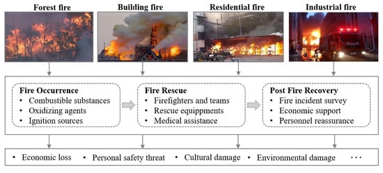
Figure 1.
Process of dealing with fire incidents.
Fire situation information plays a crucial role in guiding fire rescue operations by providing essential details such as the fire location, fire area, and fire intensity. As shown by the flame temperature data captured by sensors [1], shown in the subsequent Figure 2a, the evolution of a fire typically encompasses three distinct stages: the fire initiation stage, violent burning stage, and decay extinguishing stage. During the stage of fire initiation, the flame burns locally and erratically, accompanied by relatively low room temperatures. This phase presents an opportune time to effectively put out the fire. In the violent burning stage, the flame spreads throughout the entire room, burning steadily and causing the room temperature to rapidly rise to approximately 1000 . Extinguishing the fire becomes challenging during this stage. In the decay stage, combustible materials are consumed, and fire suppression efforts take effect. However, it is crucial to note that the fire environment undergoes rapid and dynamic changes during these stages. This renders traditional sensor-based detectors inadequate, primarily due to limitations in detection distance and susceptibility to false alarms triggered by factors such as light and dust. Moreover, these detectors are incapable of providing a visual representation of the fire scene, hindering comprehensive situational awareness.
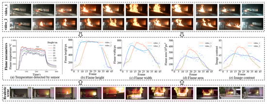
Figure 2.
Flame parameters trends during combustion. Based on two fire videos captured in the experimental scenario, flame parameters for both fire processes were computed. Similar to the sensor-based approach, flame parameters derived from visual data exhibit a three-stage combustion pattern. It is evident that the vision-based fire detection method can be extended to respond rapidly to real-world fire incidents.
Fire detection technology based on visual images offers inherent advantages. On the one hand, the portability and anti-interference of camera equipment enhance the reliability of visual fire detection. On the other hand, fire situation parameters derived from visual methods such as the flame height, width, and area are significant to fire detection and control [2]. Figure 2 illustrates the acquisition of flame situation parameters through visual fire detection technology. In the upper part of Figure 2, video_1 and video_2 represent two fire video sequences obtained in the experimental scene, in which the images were acquired through the acquisition device in Figure 3a. For the two fire videos, 45 frames of images (including three processes of combustion) were selected from each for flame parameter analysis. These image samples were subjected to the calculation process described in Figure 3b to obtain the flame height, width, and area in each frame of image, as well as the image contrast. The obtained flame parameter trends are shown in the middle of Figure 2. Initially, the size of the fire region is small. As the flames spread, the values of the flame parameters rapidly increase until they reach a stable state. After complete combustion, the flames gradually diminish, resulting in a decrease in each parameter value. Figure 2a shows the flame temperature data detected by Zhu et al. using sensors at different locations in their experimental scenario [1]. They observed that the fire process also exhibited three-stage characteristics. The five sub-figures show that the vision-based fire detection method captures flame motion patterns similar to those obtained through sensor-based methods. The visual fire detection method can be extended to realistic fire scenes, such as the home fire scene in the lower part of Figure 2. With the rapid development of computer vision technology and intelligent monitoring systems, vision-based methods offer faster response times and lower misjudgment rates than traditional sensors. The strength significantly contributes to accelerating the intelligent development of fire safety in urban areas.
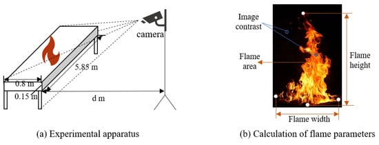
Figure 3.
Schematic diagram of experimental setup and flame parameters.
In recent years, scholars have extensively explored fire detection methods from the perspectives of image classification, object detection, and semantic segmentation. The method based on image classification aims to determine whether smoke or flame is present in an image. Zhong et al. optimized a convolutional neural network (CNN) model and combined it with the RGB color space model to extract relevant fire features [3]. Dilshad et al. proposed a real-time fire detection framework called E-FireNet, specifically designed for complex monitoring environments [4]. The object detection-based fire detection method aims to annotate fire objects in images using rectangular bounding boxes. Avazov et al. employed an enhanced YOLOv4 network capable of detecting fire areas by adapting to diverse weather conditions [5]. Fang et al. accelerated the detection speed by extracting key frames from a video and subsequently locating fires using superpixels [6]. The fire detection method based on semantic segmentation detects the fire objects’ contours by determining whether each pixel in the fire image is a fire pixel. This approach has potential to gain fine-grained parameter information (such as flame height, width, and area) in complex fire scenarios. De et al. proposed a rule-based color model, which employed the RGB and YCbCr color spaces to allow the simultaneous detection of multiple fires [7]. Wang et al. introduced an attention-guided optical satellite video smoke segmentation network that effectively suppresses the ground background and extracts the multi-scale features of smoke [8]. Ghali et al. utilized two vision-based variants of Transformer (TransUNet and MedT) to explore the potential of visible spectral images in forest fire segmentation [9]. Many fire segmentation methods have achieved notable results. However, flames exhibit variable shapes and sizes, and their edges are blurred, posing challenges to accurate segmentation. Therefore, little attention is paid to further mining fire situation information through fire segmentation.
To solve the issue, we propose a flame situation detection method called Flame-SeaFormer, which utilizes the pixel-level segmentation results of images to obtain flame parameters. By analyzing these flame parameters, valuable insights into fire propagation behavior are derived, offering crucial references for firefighting decision making and enabling the development of intelligent fire safety systems. The main contributions of this paper are as follows.
- In the context branch, squeeze-enhanced axial attention (SEA attention) squeezes the fire feature map into compact column/row information and computes self-attention to acquire the dependencies between flame pixels. In the spatial branch, the fusion block fuses low-level spatial information and high-level semantic information to obtain a more comprehensive flame feature.
- The light segmentation head maps the flame features to the pixel-level flame segmentation results using a lightweight convolution operation. Based on the flame segmentation mask, flame parameters (flame height, width, area, rate of change of flame height, and so on) are calculated to analyze the flame situation.
- The experimental results on both private and public datasets show that Flame-SeaFormer outperforms existing fire segmentation models. It extracts reliable and valid flame state information and mines flame development dynamics to support intelligent firefighting.
The rest of the paper is organized as follows. In Section 2, the related work on fire segmentation techniques is reviewed. Section 3 provides a detailed description Flame-SeaFormer. In Section 4, experiments are described to demonstrate the effectiveness of Flame-SeaFormer. Finally, conclusions are drawn in Section 5.
2. Related Work
Fire segmentation detects fire pixels in fire images by separating the foreground of smoke or flame from the background. It avoids using bounding boxes and focuses on delineating distinct boundaries. There are two categories of fire segmentation methods, feature analysis-based methods and deep learning-based methods, as shown in Figure 4.
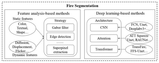
Figure 4.
Overview of relevant research on fire segmentation.
Feature analysis-based methods: Fire objects exhibit rich visual characteristics, encompassing both static features like color, texture, and shape, and dynamic features such as diffusion, displacement, and flicker [10]. Researchers have employed distinct methods to extract these features and construct comprehensive feature representations to enable effective recognition. Celik et al. employed the YCbCr color space instead of RGB to construct a universal chromaticity model for flame pixel classification [11]. Yang et al. fused two-dimensional Otst and HSI color gamut growth to handle reflections and smoke areas, efficiently segmenting suspected fire regions [12]. Ajith et al. combined optical flow, scatter, and intensity features in infrared fire images for discriminative segmentation features [13]. Chen et al. presented a fire recognition method based on enhanced color segmentation and multi-feature description [14]. The approach employs the area coefficient of variation, centroid dispersion, and circularity of images as statistics to determine the optimal threshold in fine fire segmentation. Malbog et al. compared the Sobel and Canny edge detection techniques, finding that Canny edge detection suppresses noisy edges better, achieving higher accuracy and facilitating fire growth detection [15].
Deep learning-based methods: Deep learning methods have gained prominence in computer vision across various application domains [16]. These methods utilize deep neural networks to automatically learn feature representations through end-to-end supervised training. Researchers have made substantial progress by improving classical CNN for fire segmentation. Yuan et al. proposed a CNN-based smoke segmentation method that fuses information from two paths to generate a smoke mask [17]. Zhou et al. employed Mask RCNN to identify and segment indoor combustible objects and predict the fire load [18]. Harkat et al. applied the Deeplab v3+ framework to segment flame areas in limited aerial images [19]. Perrolas et al. introduced a multi-resolution iterative tree search algorithm for flame and smoke region segmentation [20]. Wang et al. selected four classical semantic segmentation models (Unet, Deeplab v3+, FCN, and PSPNet) with two backbones (VGG16 and ResNet50) to analyze forest fires [21]. They found the Unet model with the ResNet50 backbone to have the highest accuracy. Frizzi et al. introduced a novel CNN-based network for smoke and flame detection in forests [22]. The network generates accurate flame and smoke masks in RGB images, reducing false alarms caused by clouds or haze. Attention mechanisms have also been employed, such as in ATT Squeeze Unet and Smoke-Unet, to focus on salient fire features [23,24]. Wang et al. introduced Smoke-Unet, an improved Unet model that combines an attention mechanism and residual blocks for smoke segmentation [24]. It utilizes high-sensitivity bands and remote sensing indices in multiple bands to detect forest fire smoke early. CNN-based models are effective for fire detection and segmentation, but they struggle in capturing global image information. Transformer-based models, with their self-attention mechanism, excel at capturing global features. Chali et al. employed two Transformer-based models (TransUnet and TransFire) and a CNN-based model (EfficientSeg) to identify precise fire regions in wildfires [25].
Existing fire segmentation algorithms are proficient in identifying flame pixels in video images, but accurately perceiving intricate contour semantics of flames presents a challenge, limiting the exploration of fire situation information. To address the problem, this paper employs SEA attention to capture long-range dependencies between flame pixel semantics and a fusion block to fuse low-level spatial and high-level semantic information. This refined representation of the flame’s contour enables a more detailed exploration and analysis of fire situation information.
3. Method
In the following sections, the flame situation detection task is defined. Then, the Flame-SeaFormer model is described in detail. Specifically, the general semantic segmentation model SeaFormer is introduced as an integral part of the Flame-SeaFormer framework. Moreover, a computational procedure is described to gain several static and dynamic flame parameters.
3.1. Task Definition
The flame situation detection method based on visual pixel-level segmentation aims to identify flame contours to extract flame information by determining whether each pixel in the fire image corresponds to a flame pixel.
The input of the task is a fire image captured from the original video, denoted as , where , , and represent the height, width, and number of channels of the image, respectively.
The output of the flame segmentation method SeaFormer is a mask image , where 0 corresponds to background and 1 denotes flame. From the segmentation mask, the set of contour points of the flame objects is obtained. These points serve as the basis in calculating various flame parameters. The static flame parameters include the flame height, width, and area, while the dynamic flame parameters encompass the rates of change in the flame height, width, and area. These parameters serve as outputs provided by the Flame-SeaFormer model.
3.2. The Framework of Flame-SeaFormer
Squeeze-Enhanced Axial Transformer (SeaFormer) [26] is a lightweight semantic segmentation algorithm for general domains. This model incorporates a new attention mechanism characterized by the squeeze axial and detail enhancement features, making it suitable for crafting cost-effective semantic segmentation architectures. In the context of flame segmentation, SeaFormer establishes self-adaptive global dependencies among flame pixels in the horizontal and vertical directions. This capability enables the accurate determination of flame pixels’ presence within their respective neighborhoods. This paper introduces Flame-SeaFormer, a flame situation detection model based on the pixel-level segmentation of visual images. It modifies specific parameters (such as the number of segmentation categories) of the SeaFormer model to suit the research task. The difference between Flame-SeaFormer and SeaFormer is shown in Table 1. SeaFormer focuses on the design of a semantic segmentation model, while Flame-SeaFormer places a greater emphasis on the further application of the model to analyze flame situations and explore flame combustion patterns. The overall framework of Flame-SeaFormer is illustrated in Figure 5. Firstly, for input fire video sequences containing complete combustion processes (top-left of Figure 5), the SeaFormer model (middle-left of Figure 5) extracts prominent fire features from the images and outputs pixel-level segmentation results for each image (bottom-left of Figure 5). Secondly, following the calculation of the flame parameters, static and dynamic flame parameters at different time points are obtained. Finally, based on the predicted flame parameters, flame parameter trend curves are plotted (right side of Figure 5; for spatial constraints, only static flame parameters are displayed). Then, a flame situation analysis is conducted. It consists of three main parts: the flame segmentation model SeaFormer, the inversion of static flame parameters, and the inversion of dynamic flame parameters. Subsequently, three parts of the model are introduced.

Table 1.
The differences between Flame-SeaFormer and SeaFormer.
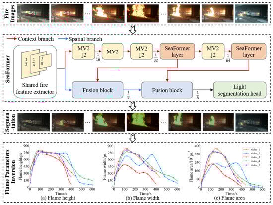
Figure 5.
The framework of multi-scale flame situation detection model Flame-SeaFormer. For input fire images, the SeaFormer model produces pixel-level segmentation results. Based on the segmentation results of fire video sequences, the flame parameter inversion section calculates static and dynamic flame parameters and then analyzes the development trends of the flames. Due to space limitations, only the trends of the flame static parameters of the five combustion processes are shown here.
3.2.1. Flame Segmentation Model: SeaFormer
As shown in Figure 5, SeaFormer consists of four modules: the shared fire feature extractor, context branch, spatial branch, and light segmentation head. Firstly, the shared fire feature extractor is employed to extract low-level fire feature maps. Secondly, both the context branch and spatial branch share the feature maps. The context branch captures global context information through axial attention, modeling features using axial attention mechanisms to obtain long-range semantic information dependencies. The spatial branch fuses low-level spatial information with high-level semantic information through the fusion block to achieve more accurate fire features. Finally, the light segmentation head employs lightweight convolution operations to map the fused features to the pixel-level fire segmentation results. The following sections will provide detailed descriptions of these four modules.
- (1)
- Shared fire feature extractor: SeaFormer adopts MobileNetV2 as the feature extraction network, leveraging its high efficiency and accuracy while operating within limited computing resources. The shared fire feature extractor consists of a regular convolution with a step size of 2 and four MobileNet blocks. Given an input image I, the extractor extracts fire features and produces a feature map , where r is the scaling factor of the feature map and is the number of channels. The operation of the fire feature extraction process is expressed aswhere FE denotes the fire feature extraction operation.
- (2)
- Context branch: The context branch is designed to capture more global and fine-grained context information from the feature map , as shown in the red branch of Figure 5. To achieve a good trade-off between segmentation accuracy and inference speed, the SeaFormer layer is introduced in the last two stages of the context branch. It consists of a squeeze-enhanced axial attention block (SEA attention) and feed-forward network (FFN), as shown in Figure 6a.
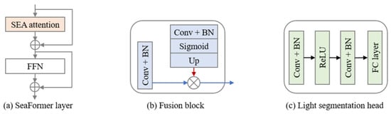
Figure 6.
Illustration of the three major modules in SeaFormer. (a) SeaFormer layer consists of SEA attention and an FFN. (b) Fusion block is utilized to fuse high-resolution fire feature maps in the spatial branch and low-resolution fire feature maps in the context branch. (c) Light segmentation head consists of two convolution layers.
As depicted in Figure 7, SEA attention employs concise squeeze axial attention for global semantic extraction, while using an efficient detail enhancement kernel based on convolution to supplement local details. Squeeze axial attention and the detail enhancement kernel are described separately.
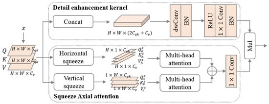
Figure 7.
Schematic illustration of SEA attention. SEA attention includes detail enhancement kernel and squeeze axial attention. The symbol ⊕ indicates an element-wise addition operation. Mul means multiplication.
Squeeze axial attention: For the feature maps obtained in the previous step for each SeaFormer layer, matrix transformation is applied to derive the query, key, and value, which is expressed as
where , , and represent the query, key, and value, respectively. , , and are learnable weight matrices. Firstly, the query matrices are horizontally and vertically compressed by averaging:
where denotes element-wise multiplication, and is a vector with all elements equal to 1. The compression operation on Q is also performed on K and V, obtaining , , , , , and . Secondly, a multi-head attention mechanism is employed to self-adaptively obtain the dependency relationships between horizontal and vertical flame pixels. Additionally, pixel-level addition is utilized to fuse the horizontal and vertical fire feature information to obtain a global fire feature. The feature value at position within this feature map is expressed as follows:
where position embedding , are introduced to make and perceive their positions in the compressed axial feature. These position embeddings are obtained through linear interpolation from the learnable parameters , , where L is a constant. In the same way, , is applied to , . Finally, a convolution operation is employed to linearly transform and adjust the input feature map in the channel dimension.
where Conv means the convolution operation.
Detail enhancement kernel: To compensate for the loss of local details caused by the compression operation, an auxiliary kernel based on convolution is introduced to enhance the spatial details. As shown in Figure 5, another query, key, and value set is obtained from the feature map x.
where , , and are learnable weight matrices. Firstly, the three matrices are concatenated in the channel dimension.
where Concat represents the concatenation operation. Then, the concatenated feature matrix is processed through a block composed of a deep convolutional layer and a batch normalization (BN) layer. This step enables the aggregation of local details from . Finally, a linear projection is employed to reduce the channel from to C, generating the detail enhancement weight. The last two steps are shown as follows:
where ReLU represents the activation function, and each convolution operation here is followed by a BN operation.
The squeeze-enhanced feature map is obtained through the multiplication of the global semantic features extracted from squeeze axial attention and the detail enhancement features derived from the detail enhancement kernel:
where Mul means the bit-wise multiplication operation. The SeaFormer layer feeds into the FFN to produce the output , enhancing the non-linear modeling capability of the model. To preserve important aspects of the original feature information and facilitate the transfer and fusion of fire feature information, residual connections are employed after the SEA attention and the FFN operations. This connection combines the learned features with the original features, ensuring the incorporation of valuable contextual information. The above operations can be summarized as follows:
where Residual means the residual connection, and FFN represents the feed-forward neural network.
- (3)
- Spatial branch: The spatial branch is designed to obtain high-resolution spatial information. Similar to the context branch, the spatial branch also operates on the feature map . However, early convolutional layers tend to contain abundant spatial information but lack higher-level semantic information. To address this, the fusion block integrates features from the context branch with the spatial branch, combining high-level fire semantic and low-level fire spatial information. As shown in the blue branch of Figure 5, the spatial branch module mainly consists of two fusion blocks. The fusion block is shown in detail in Figure 6b. In the first fusion block, the low-level feature undergoes a convolutional layer and a BN layer to generate a feature to be fused.Then, the high-level feature map derived from the context branch undergoes a sequence of operations, comprising a convolutional layer, a BN layer, and a sigmoid layer. The processed feature map is upsampled to match the high resolution via bilinear interpolation, producing a semantic weight.where Up is the upsampling operation and Sigmoid is the activation function. Finally, the semantic weight from context branch is element-wise multiplied with the feature from the spatial branch to obtain the fire feature that contains rich spatial and semantic information.The fusion block enables low-level spatial features to acquire high-level semantic information, thereby improving the accuracy of flame segmentation.
- (4)
- Light segmentation head: The output feature from the last fusion block is directly fed into the light segmentation head, as illustrated in Figure 6c. To achieve efficient inference, the segmentation head consists of two convolutional layers, each preceded by a BN layer. The feature from the first BN layer undergoes an activation layer. Subsequently, the feature is further processed by another convolutional layer, which maps the feature to the original dimensions of the input image. This process generates a semantically rich flame feature.where is the output of the second fusion block. Finally, a fully connected layer is utilized to assign a category label for each pixel.where FC denotes the fully connected operation. By aggregating the category labels of all pixels across the entire image, the flame semantic segmentation result is generated.
3.2.2. Static Flame Parameter Inversion of Individual Combustion Image
Static parameter inversion focuses on deducing static flame parameters, including the flame height, width, and area, by analyzing flame edge information based on image segmentation results. Image contrast is omitted from this analysis due to its susceptibility to external factors such as lighting and shadows.
Firstly, the coordinates of all non-zero elements are obtained from the binary mask image:
where is the position of the i-th non-zero element in the mask. Then, the coordinates are sorted in ascending order, with priority given to vertical coordinates. In the case of the same vertical coordinates, ascending order is applied to horizontal coordinates:
The sorted sequence of flame pixels is then used to extract the flame contour. Starting with the first point in , it is considered the initial point on the flame contour and subsequently removed from the sequence. The remaining points are searched, and any point with or is added to the contour coordinate set and removed from the sequence. This process continues until the sequence is empty. The extraction of contour points is expressed as
where contour represents the method of extracting contour points. denotes the initial flame contour coordinate set, which serves as the basis for the calculation of the subsequent flame width, height, and area.
The contour from the fire segmentation results may not accurately fit the real contour of the flame. To address this, a fusion process is employed to enhance the accuracy of the flame height, width, and area values. Firstly, Canny edge detection is performed on the input image I to obtain the set of edge :
For every pixel p in , if it is near the pixels in , it is added to . The process is iterated continuously until the fused contour is obtained, where n is the number of contour points.
Based on , the flame height, width, and area can be calculated. The height of a flame object is defined as the difference between the maximum and minimum values of the y-coordinates in the sequence of coordinate points along the flame’s contour:
where Y represents the set of y-coordinates of the flame contour points, max means to take the maximum value, and min means to take the minimum value. The width of a flame object is defined as the difference between the maximum and minimum values of the x-coordinates:
where X means the set of x-coordinates of the flame contour points. Finally, the polygon area method is employed to obtain the flame area :
Through the fusion operation described above, more accurate static flame parameters are obtained.
It is worth noting that in cases where the flame object in the image is fragmented or dispersed, multiple contour sequences may exist. In such a scenario, the calculation of their static parameters is carried out as follows:
where sum means summation, and d is the number of flame objects, which is equivalent to the number of contours.
3.2.3. Dynamic Flame Parameter Inversion of Time-Series Combustion Images
The dynamic flame parameter inversion of time-series combustion images involves calculating the flame height, width, and area change rates based on a sequence of consecutive images denoted as , where is length of the image sequence. For each image within this sequence, the flame contour is extracted using the previously described method. Here, represents the set of contour points of the flame object in the i-th image at time t.
For consecutive time points and , the change amounts of the flame’s height, width, and area are expressed as
where , , and denote the height, width, and area of the flame object in fire images at time t, respectively. Then, the dynamic flame parameters are obtained as follows:
where , , are the change rates of the flame height, width, and area at time t, respectively. indicates the limit at which the time interval approaches 0.
Therefore, the dynamic flame parameters are approximated by computing the differences and proportions of the flame’s height, width, and area between two adjacent frames. According to these parameters, the dynamic behavior of the flame is analyzed within a sequence of successive images.
4. Experiments
In this section, a series of experiments are described to demonstrate the effectiveness of the Flame-SeaFormer model in flame situation detection. The model’s performance is evaluated on two datasets: Our_flame_smoke (a private dataset) and FLAME (a public dataset). Widely used image segmentation models from the general domain, including FCN, Unet, Deeplab v3+, SegFormer, and GMMSeg, are chosen as comparative models. In comparison to these five methods, Flame-SeaFormer achieves superior performance in accurately detecting the state of flames.
4.1. Datasets
Our_flame_smoke and FLAME are applied to compare the segmentation performance of Flame-SeaFormer with that of other methods. The training, validation, and testing sets of the two datasets are divided at the ratio of 8:1:1, as shown in Table 2.
Table 2.
Details of two datasets.
- Our_flame_smoke: This dataset comprises 4392 fire images acquired by self-designed fire experiments, each with a resolution of 1920 × 1080. The experimental apparatus is depicted in Figure 3a. All the images in this dataset depict indoor fire scenarios, providing a comprehensive representation of the entire burning process of flames. The dataset exhibits variations in flame scale and shape, offering a diverse range of flame instances for evaluation.
- FLAME (https://ieee-dataport.org/open-access/flame-dataset-aerial-imagery-pile-burn-detection-using-drones-uavs, accessed on 24 March 2023): This dataset consists of fire images collected by drones during a pileup debris burn in an Arizona pine forest. The dataset includes 2003 flame images, each having a resolution of 3840 × 2160 pixels. Several images of the dataset are shown in the first row of Figure 8. It is worth noting that the scale of the flame objects in this dataset is relatively small as all the images were captured from an overhead view using drones.
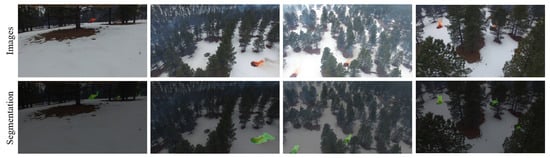 Figure 8. Several images in FLAME dataset along with their corresponding segmentation results. The first row displays the original images, while the second row shows the segmentation results. Flame pixels are highlighted in green, while background pixels remain uncolored, consistent with the original image.
4.2. Evaluation Metrics
The performance of the fire pixel-level segmentation models is evaluated in three aspects: segmentation accuracy, model complexity, and inference speed. Segmentation accuracy is quantified using metrics such as mean accuracy (), mean F1-score (), and mean intersection over union (). Model complexity analysis aims to assess the memory requirements, which are represented by the number of learnable parameters, denoted as . Inference speed refers to the number of image frames per second that the model detects, which is measured by frames per second (). The calculation processes for each metric are detailed below.
represents the average ratio of the number of correctly predicted pixels for each category to the number of true pixels in that category. It is calculated as follows:
where c is the number of categories. (true positive) represents the number of pixels correctly classified by the model as category i out of the pixels belonging to category i. (false positive) is the number of pixels incorrectly classified by the model as category i out of the pixels not belonging to category i. (true negative) indicates the number of pixels correctly classified by the model as not belonging to category i out of the pixels not belonging to category i. (false negative) is the number of pixels incorrectly classified by the model as not belonging to category i out of the pixels belonging to category i.
calculates the average F1-score for each category, as a measure of the classification or segmentation model performance. The F1-score is the harmonic mean of precision and recall. is computed by the formula
where and denote the precision and recall of class i, respectively. They are defined, respectively, as
The intersection over union () is a commonly employed evaluation metric for image segmentation tasks.It measures the ratio of the intersection area between the predicted and labeled regions to the total area covered by both regions. is expressed by the following equation:
where is the set of pixel locations within the predicted region, and represents a set of pixel locations within the true labeled region. In the case of multiple classifications, the above equation is extended to by averaging the IoU values for each category:
where is the intersection ratio of category i. The task of flame segmentation is a binary classification problem, and the pixels in the flame image are divided into two classes: flame and background. Therefore, for the above three metrics, .
The count of parameters in a model encompasses all trainable elements, including convolutional kernel weights, weights in fully connected layers, and others. For example, for a CNN model with n convolutional layers, the size of the weight matrix of each convolutional layer is and the bias vector size is ; the total number of parameters of the model is calculated as follows:
Generally, models with a smaller number of parameters tend to be lighter and exhibit faster inference speeds.
is the number of image frames processed by a model within a second. To reduce random errors, multiple images are typically averaged during actual testing. The calculation formula for is as follows:
where N denotes the number of image samples; denotes the time required for the model to process the i-th image. In this paper, .
4.3. Baselines
This paper incorporates five comparative methods to evaluate the flame segmentation performance. There are three CNN-based methods (FCN, Unet, and Deeplab v3+) and two Transformer-based methods (SegFormer and GMMSeg). These semantic segmentation methods are migrated from the generic domain to the flame segmentation domain. The baseline methods are described as follows.
- FCN (CVPR 2015) [27]: FCN (Fully Convolutional Network) is a CNN-based semantic segmentation model. It replaces fully connected layers with convolutional layers, allowing for end-to-end pixel-level classification across the entire image.
- Unet (MICCAI 2015) [28]: Unet is a segmentation method initially designed for medical images, employing an encoder–decoder architecture. It utilizes a skip connection to establish connections between the encoder and decoder layers, enabling the extraction of information from feature maps at different scales.
- Deeplab v3+ (ECCV 2018) [29]: Deeplab v3+ is an image semantic segmentation model that utilizes dilated convolution and multi-scale feature fusion. It employs dilated convolutions to expand the receptive field and incorporates the ASPP (Atrous Spatial Pyramid Pooling) module to fuse multi-scale features.
- SegFormer (NeuIPS 2021) [30]: SegFormer is a Transformer-based image segmentation model. It captures global information through a self-attention mechanism and handles features at different scales through hierarchical feature fusion.
- GMMSeg (NeuIPS 2022) [31]: GMMSeg is an image semantic segmentation model that incorporates a Gaussian mixture model and adaptive clustering. It adopts a separate mixture of Gaussians to model the data distribution of each class in the feature space. The model is trained using the adaptive clustering algorithm.
4.4. Experimental Setup
The experiments in this paper are deployed on a computer equipped with an NVIDIA GeForce RTX 3090 GPU (Nvidia Corporation, Santa Clara, CA, USA).The Pytorch deep learning framework is employed for model training, leveraging the CUDA, Cudnn, and OpenCV libraries to facilitate the training and testing of the flame segmentation model. The network is optimized using the Adam optimizer. The initial learning rate is 0.0002 and the weight decay is 0.01. In the two datasets, a batch size of 6 is employed during the training process. The training images are randomly scaled and then cropped to the fixed size of 512 × 512.
4.5. Experimental Result and Analysis
This subsection presents a comprehensive performance analysis of Flame-SeaFormer, encompassing both quantitative and qualitative evaluations. Firstly, the segmentation results of Flame-SeaFormer and the baselines are shown from the global and local perspectives of flame burning. The results reveal that Flame-SeaFormer exhibits superior suitability for the pixel-level flame segmentation task. Secondly, the case study section clearly shows the visualization results of the Flame-SeaFormer model on multi-scale, small-scale, and negative samples. Then, the Flame-SeaFormer method is employed to estimate static flame parameters, such as the flame height, width, and area, in individual fire images. Finally, dynamic flame parameters, the change rates of the flame height, width, and area, are analyzed based on the sequence of flame-burning images to achieve multi-scale flame situation detection and analysis.
4.5.1. Visual Segmentation Results of the Global Flame-Burning Process
The comparative results of global visual segmentation between Flame-SeaFormer and other methods on two datasets are shown in Table 3 and Table 4, respectively. In particular, the results of the metric for each model are visualized in Figure 9. Through careful observation, the following information is obtained.
Table 3.
Comparation results on Our_flame_smoke (testing set).
Table 4.
Comparation results on FLAME (testing set).
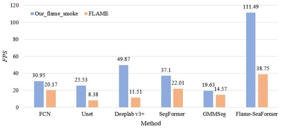
Figure 9.
The results on the two datasets.
On the Our_flame_smoke dataset, GMMSeg achieves the highest segmentation accuracy, surpassing Deeplab v3+ (the lowest performer) by 1.99%, 1.18%, and 2.15% in terms of , , and , respectively. However, GMMSeg relies on a Gaussian distribution for pixel modeling, leading to the highest parameter count and the longest inference time. Flame-SeaFormer ranks third in the segmentation accuracy metrics, with the differences between GMMSeg and Flame-SeaFormer being relatively minor. Notably, Flame-SeaFormer exhibits a significant advantage in terms of , processing 111 frames per second. Compared with GMMSeg, Flame-SeaFormer offers a tenfold increase in inference speed with only a 10% reduction in parameter count, at the cost of a mere 0.73% decrease in . When compared to SegFormer, the second highest ranked model, Flame-SeaFormer achieves a nearly three times faster inference speed while losing only 0.11% . In scenarios requiring a swift response to fire incidents, the model’s response speed is the most critical metric, which needs to be balanced with the inference performance. Overall, Flame-SeaFormer provides the best choice for multi-scale fire segmentation tasks, striking the best balance between accuracy and speed.
Regarding the FLAME dataset, SegFormer emerges as the top performer in segmentation accuracy, attaining an of 91.06%. Flame-SeaFormer secures second place in terms of , , and , trailing SegFormer by merely 0.12% in the metric. In comparison to the worst-performing model, FCN, Flame-SeaFormer improves by 6.52%, 5.25%, and 7.78% across the three segmentation accuracy metrics. In terms of inference speed, Flame-SeaFormer still maintains its dominance, exhibiting twice the inference speed and one fifth of the model complexity when compared to SegFormer, at the expense of only a 0.12% decrease in . Collectively, when dealing with small-scale flame images, Flame-SeaFormer still exhibits excellent and fast segmentation performance.
In summary, Flame-SeaFormer demonstrates superior overall performance compared to the baselines across the two datasets. Meanwhile, its inference accuracy and speed align with the requirements of real-time fire information perception. This achievement is attributed to the SEA attention, which integrates crucial spatial information, facilitating the enhancement of local details and effective fusion of global contextual information. Moreover, the comparative analysis of the model’s performance on two datasets reveals challenges in accurately segmenting flames within the FLAME dataset. These challenges stem from the concealed, diminutive nature of small-sized flame targets and their dispersed distribution across multiple points.
4.5.2. Visual Segmentation Results of the Local Flame-Burning Stage
As described in the Introduction, this paper divides the flame combustion process into three stages: the initial fire, the violent burning, and the decaying extinguishing stages. The images on the FLAME dataset were captured from a top-down perspective using a drone, and it is difficult to distinguish the corresponding flame-burning stage of each image. Consequently, a local analysis of FLAME is omitted from this study. Instead, the focus is on evaluating the performance of Flame-SeaFormer and other methods on the Our_flame_smoke dataset, specifically concerning the visual segmentation results at each stage. The segmentation accuracy metric is selected as the evaluation criterion. The results are presented in Table 5, with the stages conveniently labeled as early, midterm, and later. Furthermore, the metric for each stage is visualized in a histogram shown in Figure 10. Through observation, the following information is obtained.
Table 5.
Segmentation results of the three stages of flame combustion on Our_flame_smoke.
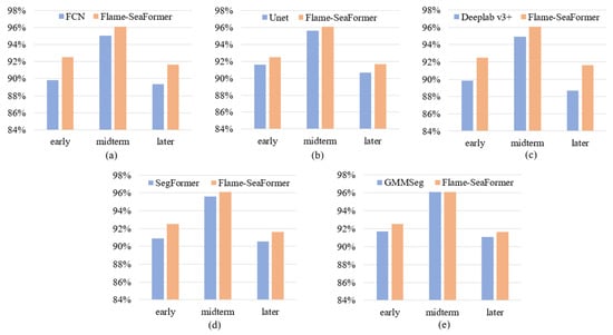
Figure 10.
The results of the three stages of flame combustion. (a) FCN vs. Flame-SeaFormer. (b) Unet vs. Flame-SeaFormer. (c) Deeplab v3+ vs. Flame-SeaFormer. (d) SegFormer vs. Flame-SeaFormer. (e) GMMSeg vs. Flame-SeaFormer.
Flame-SeaFormer exhibits superior segmentation performance across the three distinct stages of flame combustion. Compared to Unet, which is considered the top-performing model in the CNN architecture category, Flame-SeaFormer achieves significant improvements of 0.91%, 0.49%, and 0.96% in for the respective stages. In comparison to GMMSeg, the top-performing Transformer-based model, Flame-SeaFormer showcases comparable performance during the intense flame-burning phase, while outperforming GMMSeg by 0.83% and 0.59% in for the fire initiation and decay extinction phases, respectively. The analysis of the flame-burning stages reveals distinct characteristics. During the initial stage, there is an observable increase in the scale of the flames, while, in the intense combustion phase, the flames spread slowly and remain stable, reaching their maximum scale. In the flame extinction stage, the flames gradually diminish, resulting in a reduction in scale. There exist flame objects of varying shapes and scales during the combustion process. Flame-SeaFormer has excellent segmentation quality for multi-scale flame targets. Apparently, the SEA attention and fusion block enable the model to adaptively capture low-level spatial and high-level semantic features in flames of different scales. This capability allows the model to perceive flame edge details and enhance the accuracy of flame parameter estimation.
4.5.3. Case Analysis
To demonstrate the superiority of the Flame-SeaFormer model, some images from each of the two datasets are selected for inference to visualize the quantitative segmentation results. The images from the FLAME dataset are all UAV overhead shots where the flame targets are hidden and small, making it difficult to distinguish the corresponding flame-burning stages. Therefore, small-scale flame segmentation result analysis is performed on this dataset. The images in Our_flame_smoke are derived from multiple fire videos that contain the complete burning process, and thus the analysis of the multi-scale flame segmentation results is performed on the Our_flame_smoke dataset. Further, several negative samples (i.e., images without flame targets) are chosen from the two datasets to evaluate the interference resistance capabilities of Flame-SeaFormer. In the following, small-scale flame segmentation analysis, multi-scale flame segmentation analysis, and negative sample segmentation analysis are described in detail.
Four original images containing different numbers of fire targets are selected from the FLAME dataset for small-scale flame segmentation analysis. Employing the trained model weights for inference, the qualitative segmentation results of the four images are shown in the second row of Figure 8. Through the analysis, it can be seen that Flame-SeaFormer has superior performance in small target flame pixel segmentation. Meanwhile, Flame-SeaFormer demonstrates a certain degree of flame recognition capability, even in cases of occluded flames.
Several fire images representing three combustion stages in the Our_flame_smoke dataset are selected for inference. The segmentation results are visually presented in Figure 11, from which several key observations can be drawn. During the initial and decaying stages, where weak flame targets exist and the number of flame pixels is relatively low, Flame-SeaFormer exhibits exceptional sensitivity and recognition accuracy in detecting subtle flame regions. In the intense flame-burning phase, characterized by visible and large-scale flames, the model accurately identifies flame regions by leveraging the global interdependence among multiple pixel points, enabling precise mapping between fine-grained pixels and flame semantics. Furthermore, Flame-SeaFormer effectively avoids misclassifying light shadows refracted by the flame as flames, demonstrating its ability to automatically filter interference features and utilize valid flame information. In summary, consistent with the quantitative results in Table 5, Flame-SeaFormer identifies and distinguishes flame regions of diverse scales throughout the entire flame-burning process. The finding validates the model’s potential in quantifying flame development and supports its application in improving urban fire safety.
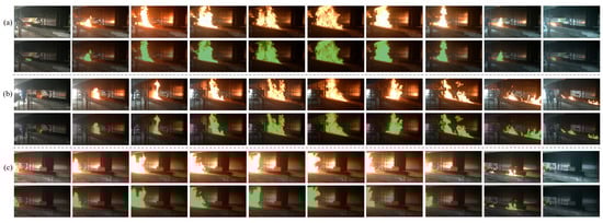
Figure 11.
Multi-scale flame segmentation results on Our_flame_smoke dataset. (a–c) represent the original image sequences of three burning processes, respectively. The next line of each sequence corresponds to the flame segmentation result. The flame pixels are highlighted in green, while the background pixels are uncolored and consistent with the original image.
Two representative negative samples from each of the two datasets are selected for inference, and the segmentation results are shown in Figure 12. For the two images from Our_flame_smoke, the color of the fire extinguisher in Figure 12a has similarity with the flame in the color hierarchy, and the refracted light shadows on the tin in Figure 12b are also confused with firelight. Nevertheless, Flame-SeaFormer demonstrates the adaptive capability to effectively filter out interfering features associated with fire-like objects. The images from the FLAME dataset feature diverse non-fire objects with varying shapes. However, Flame-SeaFormer remains resilient to the complexities of the environment. From the above analysis, it is evident that Flame-SeaFormer exhibits strong anti-interference ability.
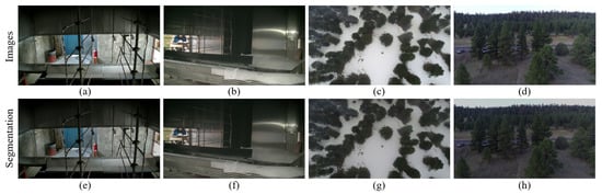
Figure 12.
Segmentation results of negative samples. (a–d) are four negative samples selected from two datasets, where (a,b) are from the Our_flame_smoke dataset. (c,d) are from the FLAME dataset. (e–h) are their corresponding segmentation results.
4.5.4. Inversion Results of Static Flame Parameters
Based on the preceding analysis, Flame-SeaFormer is selected to invert the static flame parameters: flame height, width, and area. Five combustion processes are chosen for analysis, capturing one image frame every 1 s. The inversion results are depicted in Figure 13. Due to variations in the duration of the different combustion processes, the endpoint coordinates of the five curves differ.
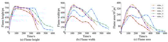
Figure 13.
The static flame parameters of a flame in five videos.
Among the three subplots, the flame height exhibits the most distinct pattern. From 0–100 s, the flames in the five combustion experiments burned rapidly. The values of the three static flame parameters reach peaks at around 100 s. Subsequently, each static parameter remains stable or fluctuates slightly, indicating the vigorous combustion stage. After 300 s, groups 1, 3, 4, and 5 entered the decay and extinction phase, with flames gradually decreasing in intensity. The second experiment lasted longer, entering the third stage of combustion at around 400 s. Flame-SeaFormer accurately calculates reasonable flame parameters for all individual images at different combustion moments. A typical study conducted by Mangs et al. investigated the upward spread of a flame on an FRNC N2XCH cable using a thermocouple [32]. The burn length (i.e., flame height) was treated as a function of time, with the curve shown in Figure 14. A comparison between the image-based Flame-SeaFormer model’s results and the physical device’s measurements in Figure 14 reveals a consistent flame development pattern. The consistency provides strong evidence for the reliability and efficiency of the gained flame-burning parameters by the model. In urgent fire scenarios, Flame-SeaFormer shows great promise for the real-time sensing of multi-scale flame information and the analysis of flame propagation properties.
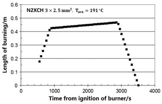
Figure 14.
Flame height on an FRNC N2XCH cable pre-heated to T = 191 .
4.5.5. Inversion Results of Dynamic Flame Parameters
Utilizing the obtained values of the flame height, width, and area parameters from the previous section, the dynamic flame parameters (rates of change in flame height, width, and area) are calculated. The rates of change are computed at 1-s intervals and and visualized in Figure 15. Positive rates of change indicate gradual increases in each static flame parameter, signifying flame spread in the vertical and horizontal directions. A rate of change of 0 indicates relatively stable flame shapes and complete burning. Conversely, negative values indicate a decrease in flame regions. According to Figure 15, some observations are made as follows.
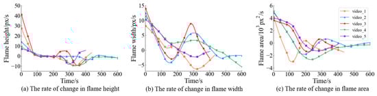
Figure 15.
The dynamic flame parameters of a flame in five videos.
During the initial stage of the fire, the flame spreads rapidly, with the spreading rate gradually decreasing before reaching the violent burning stage. In the intense burning stage, the rates of change remain close to 0 or stable. As the flame decays, the rate of change becomes negative, resulting in the contraction of the flame height, width, and area. Chen et al. studied the evolution of ammonia/air flame fronts and laminar flame parameters influenced by buoyancy [33]. The red and blue curves in Figure 16 depict the rate of increase for the flame in the height and width directions over time during the early and midterm stages of flame propagation. After ignition, the flame exhibits vertical expansion, with the flame generally growing at a higher rate in height than in width. After a certain time, the flame reaches a smooth burning state. Although the figure does not display the rates of change during the flame extinction phase, it is reasonable to infer that the flame intensity gradually decreases during the later stages of combustion. These findings further support the potential of Flame-SeaFormer in utilizing fire images to explore flame development, specifically focusing on the analysis of evolving flame patterns. Clearly, the flame parameters calculated from the Flame-SeaFormer model are reasonably plausible.
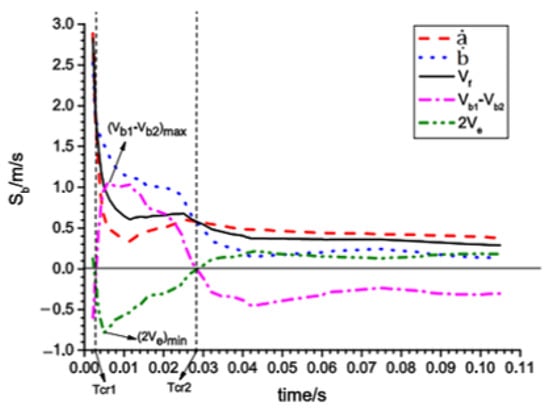
Figure 16.
Variations in axial length under increasing velocity with time in ammonia/air mixture.
5. Conclusions
Flames in fire incidents pose challenges regarding precise segmentation and obtaining reliable flame situation parameters due to their variable shapes and sizes. To address this problem, this paper proposes the Flame-SeaFormer model for the pixel-level segmentation of multi-scale flame images, enabling the analysis of the flame-burning state and the extraction of static and dynamic flame parameters. Firstly, in the context branch, SEA attention models the fire feature map along the horizontal and vertical directions, facilitating self-attention mechanisms to capture long-range dependencies among flame pixel semantics. Secondly, in the spatial branch, the fusion block fuses low-level spatial information with high-level semantic information to refine the flame edges and enhance the flame information. Finally, the light segmentation head segments the feature map containing global fire information at the pixel level in a very short time. Leveraging the flame segmentation results, the contours of flames are obtained, facilitating the extraction of both static flame parameters (flame height, width, and area) and dynamic flame parameters (change rates of flame height, width, and area). The experimental results demonstrate that Flame-SeaFormer achieves an excellent balance between inference accuracy and speed, outperforming existing fire segmentation models. Its ability to provide dependable fire status information and mine flame dynamics will help firefighters to make accurate decisions and drive the development of smart cities.
From the experimental findings, our work still has limitations in two aspects. On the one hand, although the Flame-SeaFormer model achieves the best balance between segmentation accuracy and speed, there remains room for improvement in the segmentation accuracy, particularly in enhancing its ability to delineate boundary flame pixels. On the other hand, Flame-SeaFormer is only applied in self-constructed experimental scenarios and forest fire scenarios. The exploration of flame parameter analysis within more realistic fire scenarios, such as common urban building fires, remains an uncharted domain. Addressing these limitations, future work will primarily focus on refining the model architecture and broadening its application scope. In terms of model architecture design, the fire feature extraction method could be optimized by combining counterfactual assumptions and removing confounding elements in the data to further reduce the missed segmentation of flames. Concerning the extension of the application scenarios, more fire images of real scenarios could be collected and annotated, facilitating model training on diverse datasets to enhance its generalization capacity.
Author Contributions
Conceptualization, X.W.; methodology, X.W., M.L. and Y.C.; validation, X.W., Q.L., Y.C. and H.Z.; formal analysis, X.W. and M.L.; investigation, M.L. and Y.C.; resources, X.W. and Q.L.; data curation, X.W. and Q.L.; writing—original draft preparation, M.L. and Y.C.; writing—review and editing, X.W., M.L., Q.L. and H.Z.; visualization, M.L.; supervision, X.W., Q.L. and H.Z.; project administration, X.W.; funding acquisition, X.W. All authors have read and agreed to the published version of the manuscript.
Funding
This work was funded by the National Science Foundation of China (Grant No. 72204155, Grant No. U2033206), the Natural Science Foundation of Shanghai (Grant No. 23ZR1423100), and the Project of Civil Aircraft Fire Science and Safety Engineering Key Laboratory of Sichuan Province (Grant No. MZ2022KF05, Grant No. MZ2022JB01).
Institutional Review Board Statement
Not applicable.
Informed Consent Statement
Not applicable.
Data Availability Statement
The FLAME dataset is available from https://ieee-dataport.org/open-access/flame-dataset-aerial-imagery-pile-burn-detection-using-drones-uavs (accessed on 24 March 2023). Our self-built dataset (Our_flame_smoke) will be made publicly available after publication.
Conflicts of Interest
The authors declare no conflict of interest.
References
- Zhu, P.; Luo, S.; Liu, Q.; Shao, Q.; Yang, R. Effectiveness of aviation kerosene pool fire suppression by water mist in a cargo compartment with low-pressure environment. J. Tsinghua Univ. (Sci. Technol.) 2022, 62, 21–32. [Google Scholar]
- Chen, X.; Hopkins, B.; Wang, H.; O’Neill, L.; Afghah, F.; Razi, A.; Fulé, P.; Coen, J.; Rowell, E.; Watts, A. Wildland Fire Detection and Monitoring Using a Drone-Collected RGB/IR Image Dataset. IEEE Access 2022, 10, 121301–121317. [Google Scholar] [CrossRef]
- Zhong, Z.; Wang, M.; Shi, Y.; Gao, W. A convolutional neural network-based flame detection method in video sequence. Signal Image Video Process. 2018, 12, 1619–1627. [Google Scholar] [CrossRef]
- Dilshad, N.; Khan, T.; Song, J. Efficient Deep Learning Framework for Fire Detection in Complex Surveillance Environment. Comput. Syst. Sci. Eng. 2023, 46, 749–764. [Google Scholar] [CrossRef]
- Avazov, K.; Mukhiddinov, M.; Makhmudov, F.; Cho, Y.I. Fire detection method in smart city environments using a deep-learning-based approach. Electronics 2021, 11, 73. [Google Scholar] [CrossRef]
- Fang, Q.; Peng, Z.; Yan, P.; Huang, J. A fire detection and localisation method based on keyframes and superpixels for large-space buildings. Int. J. Intell. Inf. Database Syst. 2023, 16, 1–19. [Google Scholar] [CrossRef]
- De Sousa, J.V.R.; Gamboa, P.V. Aerial forest fire detection and monitoring using a small uav. KnE Eng. 2020, 5, 242–256. [Google Scholar]
- Wang, T.; Hong, J.; Han, Y.; Zhang, G.; Chen, S.; Dong, T.; Yang, Y.; Ruan, H. AOSVSSNet: Attention-guided optical satellite video smoke segmentation network. IEEE J. Sel. Top. Appl. Earth Obs. Remote Sens. 2022, 15, 8552–8566. [Google Scholar] [CrossRef]
- Ghali, R.; Akhloufi, M.A.; Jmal, M.; Souidene Mseddi, W.; Attia, R. Wildfire segmentation using deep vision transformers. Remote Sens. 2021, 13, 3527. [Google Scholar] [CrossRef]
- Chen, Y.; Xu, W.; Zuo, J.; Yang, K. The fire recognition algorithm using dynamic feature fusion and IV-SVM classifier. Clust. Comput. 2019, 22, 7665–7675. [Google Scholar] [CrossRef]
- Celik, T.; Demirel, H. Fire detection in video sequences using a generic color model. Fire Saf. J. 2009, 44, 147–158. [Google Scholar] [CrossRef]
- Yang, L.; Zhang, D.; Wang, Y.H. A new flame segmentation algorithm based color space model. In Proceedings of the 2017 29th Chinese Control And Decision Conference (CCDC), Chongqing, China, 28–30 May 2017; pp. 2708–2713. [Google Scholar]
- Ajith, M.; Martínez-Ramón, M. Unsupervised segmentation of fire and smoke from infra-red videos. IEEE Access 2019, 7, 182381–182394. [Google Scholar] [CrossRef]
- Chen, X.; An, Q.; Yu, K.; Ban, Y. A novel fire identification algorithm based on improved color segmentation and enhanced feature data. IEEE Trans. Instrum. Meas. 2021, 70, 5009415. [Google Scholar] [CrossRef]
- Malbog, M.A.F.; Lacatan, L.L.; Dellosa, R.M.; Austria, Y.D.; Cunanan, C.F. Edge detection comparison of hybrid feature extraction for combustible fire segmentation: A Canny vs. Sobel performance analysis. In Proceedings of the 2020 11th IEEE Control and System Graduate Research Colloquium (ICSGRC), Shah Alam, Malaysia, 8 August 2020; pp. 318–322. [Google Scholar]
- Voulodimos, A.; Doulamis, N.; Doulamis, A.; Protopapadakis, E. Deep learning for computer vision: A brief review. Comput. Intell. Neurosci. 2018, 2018, 7068349. [Google Scholar] [CrossRef] [PubMed]
- Yuan, F.; Zhang, L.; Xia, X.; Wan, B.; Huang, Q.; Li, X. Deep smoke segmentation. Neurocomputing 2019, 357, 248–260. [Google Scholar] [CrossRef]
- Zhou, Y.C.; Hu, Z.Z.; Yan, K.X.; Lin, J.R. Deep learning-based instance segmentation for indoor fire load recognition. IEEE Access 2021, 9, 148771–148782. [Google Scholar] [CrossRef]
- Harkat, H.; Nascimento, J.M.; Bernardino, A.; Thariq Ahmed, H.F. Assessing the impact of the loss function and encoder architecture for fire aerial images segmentation using deeplabv3+. Remote Sens. 2022, 14, 2023. [Google Scholar] [CrossRef]
- Perrolas, G.; Niknejad, M.; Ribeiro, R.; Bernardino, A. Scalable fire and smoke segmentation from aerial images using convolutional neural networks and quad-tree search. Sensors 2022, 22, 1701. [Google Scholar] [CrossRef]
- Wang, Z.; Peng, T.; Lu, Z. Comparative research on forest fire image segmentation algorithms based on fully convolutional neural networks. Forests 2022, 13, 1133. [Google Scholar] [CrossRef]
- Frizzi, S.; Bouchouicha, M.; Ginoux, J.M.; Moreau, E.; Sayadi, M. Convolutional neural network for smoke and fire semantic segmentation. IET Image Process. 2021, 15, 634–647. [Google Scholar] [CrossRef]
- Zhang, J.; Zhu, H.; Wang, P.; Ling, X. ATT squeeze U-Net: A lightweight network for forest fire detection and recognition. IEEE Access 2021, 9, 10858–10870. [Google Scholar] [CrossRef]
- Wang, Z.; Yang, P.; Liang, H.; Zheng, C.; Yin, J.; Tian, Y.; Cui, W. Semantic segmentation and analysis on sensitive parameters of forest fire smoke using smoke-unet and landsat-8 imagery. Remote Sens. 2022, 14, 45. [Google Scholar] [CrossRef]
- Ghali, R.; Akhloufi, M.A.; Mseddi, W.S. Deep learning and transformer approaches for UAV-based wildfire detection and segmentation. Sensors 2022, 22, 1977. [Google Scholar] [CrossRef] [PubMed]
- Wan, Q.; Huang, Z.; Lu, J.; Yu, G.; Zhang, L. SeaFormer: Squeeze-enhanced Axial Transformer for Mobile Semantic Segmentation. In Proceedings of the Eleventh International Conference on Learning Representations, ICLR 2023, Kigali, Rwanda, 1–5 May 2023. [Google Scholar]
- Long, J.; Shelhamer, E.; Darrell, T. Fully convolutional networks for semantic segmentation. In Proceedings of the IEEE Conference on Computer Vision and Pattern Recognition, Boston, MA, USA, 7–12 June 2015; pp. 3431–3440. [Google Scholar]
- Ronneberger, O.; Fischer, P.; Brox, T. U-net: Convolutional networks for biomedical image segmentation. In Proceedings of the Medical Image Computing and Computer-Assisted Intervention—MICCAI 2015: 18th International Conference, Munich, Germany, 5–9 October 2015; Springer: Cham, Switzerland, 2015; pp. 234–241. [Google Scholar]
- Chen, L.C.; Zhu, Y.; Papandreou, G.; Schroff, F.; Adam, H. Encoder-decoder with atrous separable convolution for semantic image segmentation. In Proceedings of the European Conference on Computer Vision (ECCV), Munich, Germany, 8–14 September 2018; pp. 801–818. [Google Scholar]
- Xie, E.; Wang, W.; Yu, Z.; Anandkumar, A.; Alvarez, J.M.; Luo, P. SegFormer: Simple and efficient design for semantic segmentation with transformers. Adv. Neural Inf. Process. Syst. 2021, 34, 12077–12090. [Google Scholar]
- Liang, C.; Wang, W.; Miao, J.; Yang, Y. GMMSeg: Gaussian Mixture based Generative Semantic Segmentation Models. In Proceedings of the NeurIPS 2022, New Orleans, LA, USA, 28 November–9 December 2022. [Google Scholar]
- Mangs, J.; Hostikka, S. Vertical flame spread on charring materials at different ambient temperatures. Fire Mater. 2013, 37, 230–245. [Google Scholar] [CrossRef]
- Chen, X.; Liu, Q.; Jing, Q.; Mou, Z.; Shen, Y.; Huang, J.; Ma, H. Flame front evolution and laminar flame parameter evaluation of buoyancy-affected ammonia/air flames. Int. J. Hydrogen Energy 2021, 46, 38504–38518. [Google Scholar] [CrossRef]
Disclaimer/Publisher’s Note: The statements, opinions and data contained in all publications are solely those of the individual author(s) and contributor(s) and not of MDPI and/or the editor(s). MDPI and/or the editor(s) disclaim responsibility for any injury to people or property resulting from any ideas, methods, instructions or products referred to in the content. |
© 2023 by the authors. Licensee MDPI, Basel, Switzerland. This article is an open access article distributed under the terms and conditions of the Creative Commons Attribution (CC BY) license (https://creativecommons.org/licenses/by/4.0/).