Research on a Time Series Data Prediction Model Based on Causal Feature Weight Adjustment

Abstract

As the Information Age brings people an amount of data, research on data prediction has been widely concerned. Time series data, a sequence of data points collected over an interval of time, are very common in many areas such as weather forecasting, stock markets, and so on. Thus, research on time series data prediction is of great significance. Traditional prediction methods are usually based on correlations between data points, but correlations do not always reflect the relationship exactly within the data. In this paper, we propose the LiNGAM Weight Adjust–LSTM (LWA-LSTM) algorithm, which combines a causality discovery algorithm, feature weight adjustment, and a deep neural network for time series data prediction. Several stocks in the Chinese stock market were selected and the algorithm was used to predict the stock price. Comparing the prediction effect of the model with that of the LSTM model alone, the results show that the LWA-LSTM model can find the stable relationship between the data better and has fewer prediction errors.

1. Introduction

Time series data, also referred to as time-stamped data, are a sequence of data points indexed in time order. They are widely present in our daily lives, such as in weather forecasting, stock markets, and other fields. Nowadays, the accurate prediction and analysis of time series data have become a hot research topic in the field of artificial intelligence. Stock prices are typical time series data. Many scholars have carried out research on stock price forecasting due to its potential high returns. However, since stock data are often unstable and noisy and are greatly affected by international relations and national policies, the prediction of stock data has always been a challenging problem. Therefore, we take stock price data as an example to study the forecast of time series data, proposing a new method to improve prediction accuracy.

Thanks to the extensive research scholars have conducted, many effective methods have been proposed. Before the advent of machine learning, statistical approaches were widely tried and tested. The Exponential Smoothing Model [1] uses the exponential window function to smooth time series data and then analyze them. The ARMA [2] is another popular technique for stock market analysis, which combines the Auto-Regressive (AR) model, which models the momentum and mean reversion effects observed in trading markets, and the Moving Average (MA) model, which tries to capture the shock effects observed. The ARIMA [3] is a natural extension of the ARMA model that can reduce a non-stationary series to a stationary series. Machine learning methods include random forest [4], xgboost [5], and support vector machine [6]. As neural network models show their great potential, more and more deep learning models have been proposed for stock price prediction, based on RNN [7], CNN [8], LSTM [9], GRU [10], and so on. We will introduce some of them in the next chapter.

We found that when using machine learning methods for time series prediction, the choice of features greatly affects the prediction performance. Existing methods often can only find correlations within variables. As we all know, correlation differs from causality, which is a more essential and thus more stable and reliable relationship in time series data. Therefore, it is of great significance to explore the causal relationship between stock price data for forecasting.

To achieve this, we devised an effective novel method. First, we selected a set of stock factors as features and used a causal discovery algorithm to model the causal relationship between these features and the objective. Next, we adjusted the weights of the features that had a causal relationship with the objective. Finally, we used the weighted feature set as input to predict the stock price with the LSTM neural network.

The contributions of this paper are as follows: (1) To the best of our knowledge, we apply the causal discovery algorithm based on a structural causal model to the stock price prediction for the first time. (2) Based on the LiNGAM algorithm and LSTM algorithm, we propose LWA-LSTM, which is capable of discovering causality and predicting time series data. (3) We find that there is a causal relationship rather than a correlation between many features and the stock price to be predicted. (4) LWA-LSTM achieved excellent performance when tested on real stock data. Our work validates the potential for adding causality and causal weight adjustment to produce more reliable and accurate predictions for such tasks.

This paper is organized as follows. Section 2 introduces the relevant work. Section 3 provides a detailed description of the LWA-LSTM method we devised. In Section 4, we show the experiment settings and results. Finally, in Section 5, we summarize our work and look forward to the future.

2. Related Work

For a long time, people have been disputing whether the stock market can be predicted. The efficient market hypothesis proposed by Fama [11] holds that information is efficient; that is, new information can be quickly reflected in asset prices, so future stock prices cannot be predicted based on historical information. Goyal and Welch [12] systematically investigated the empirical real-world out-of-sample performance of plain linear regressions to predict the equity premium and found that none of the popular variables worked. Goyal, Welch, and Zafirov [13] reexamined whether 29 variables from 26 papers published after Goyal and Welch, as well as the original 17 variables, were useful in predicting the equity premium in-sample and out-of-sample. The results show that the predictive performance of popular variables is still disappointing. However, because the efficient market hypothesis has very strong assumptions, it is difficult to satisfy in the real world. With the development of computer technology, various forecasting methods other than linear regression have been enriched. Therefore, many researchers still make stock forecasts for high returns. Fundamental analysis and technical analysis have been used for decades. The traditional stock forecasting method is generally based on statistical models, establishing a linear model between stock features and stock price. Li et al. [14] built an ARIMA model using the monthly closing price of the SSE Composite Index to predict the closing price in three months, verifying the accuracy of the ARIMA model in short-term prediction. Such methods achieved good results with very few model parameters and low computational complexity. However, they often assume data with linearity, stationarity, and normality, which is often too strict. There are many complex nonlinear relationships between stock variables.

Thanks to the massive data recorded in the financial market, the use of machine learning in stock markets is growing rapidly. Various algorithms such as support vector machines, perceptrons, artificial neural networks, and decision trees have been applied to stock price prediction to improve the accuracy.

Kim [15] applied a support vector machine to stock prediction, and experiments showed that the method outperformed traditional neural networks. Qiu [16] used artificial neural networks combined with global search techniques (GA/SA) to make predictions. Although these methods have been greatly improved compared with the traditional methods, complex feature engineering and poor model scalability have always troubled researchers. Deep learning has now become the most popular solution for most AI problems. Many researchers use RNNs to make stock price predictions. Although Recurrent Neural Networks (RNNs) possess internal memory and feedback connections, making them capable of handling sequences of arbitrary length, the model’s performance is heavily compromised as the input length increases. Furthermore, excessively long inputs can lead to issues of vanishing or exploding gradients, making the training process extremely challenging. The LSTM (Long Short-Term Memory) model was developed based on the RNN. LSTM incorporates three control units: the forget gate, the input gate, and the output gate. These units effectively enhance the model’s ability to handle long-range dependencies in sequential data. In addition to approximating complex non-linear relationships, LSTM also offers advantages such as high accuracy, strong learning capability, robustness, and fault tolerance. Catalin [17] designed stock forecasting models based on LSTM and CNN, respectively, and built a stock trading strategy with prediction results. Sellvin et al. [18] proposed three stock prediction models based on the CNN, RNN, and LSTM respectively, and compared their performance by predicting the stock price of listed companies. Chen et al. [19] proposed a stock price trend prediction model (TPM) based on the encoder–decoder mechanism. This proposed method consists of two phases. First, it applied a piece-wise linear regression method (PLR) (which extracts long-term temporal features) and a CNN (which extracts short-term spatial market features) as a dual feature extraction method. Second, an encoder–decoder framework formed by an LSTM was applied to select and merge relevant features and then perform trend prediction. Among the multiple advantages of transformers, the ability to capture long-range dependencies and interactions is especially attractive for time series modeling, leading to exciting progress in various time series applications. By highlighting their advantages and limitations, Wen et al. [20] comprehensively and systematically summarize transformers’ work on the latest advances in time series data modeling. Liu et al. [21] proposed a capsule network based on a transformer. They captured semantic features with a transformer encoder and text structure information with capsule networks, thereby extracting features from the text on social media for stock predictions. Lin et al. [22] proposed a new deep learning method for time series prediction, SSDNet. This approach combines the transformer architecture with a state-space model to provide probabilistic and interpretable predictions. The paper evaluates the performance of SSDNet on five datasets, showing that SSDNet is an effective method in terms of accuracy and speed. Gupta et al. [23] proposed the StockNet model based on GRU with a new data augmentation approach to overcome the issue of overfitting. Hossain et al. [24] propose a deep learning-based hybrid model that consists of two well-known DNN architectures: LSTM and GRU. The approach involves passing the input data to the LSTM network to generate a first-level prediction and then passing the output of the LSTM layer to the GRU layer to obtain the final prediction. A novel deep-learning approach to predict the stock market using both historical stock prices and financial news data can be found in Lien Minh et al. [25]. In this study, mainly two novel approaches were used. First, a two-stream gated recurrent unit (TGRU) model for stock price trend forecasting; second, a sentiment Stock2Vec embedding model associated with financial news data as well as a sentiment dictionary. The proposed network achieved a mean squared error (MSE) of 0.00098 in prediction, outperforming previous neural network approaches. Shah et al. [26] proposed AutoAI for time series forecasting (AutoAI-TS). The model can use classical statistical models, machine learning (ML) models, and deep learning models to create prediction pipelines and use the T-Daub mechanism to select the best pipeline for prediction.

Existing predictive models often only reveal the underlying correlation relationships rather than causal relationships between features and stock prices. A common causal analysis method for time series data is the Granger causality test proposed by C.W.J. Granger [27], which promoted econometrics. Hiemstra and Jones [28] tested the nonlinear causality between transaction volume and returns, confirming the validity of the Granger causality test. With the linear and non-linear Granger causality tests, Param et al. [29] found that there is a significant two-way causality between daily stock returns and trading volume in Korea. Using the same technique, Zhuo et al. [30] found that the Michigan Consumer Sentiment Index has a causal relationship with the consumption trend in the United States. However, there is no solid causal theory foundation for the Granger causality test. It has been recognized that proving causality requires counterfactual reasoning. A causal relationship is more stable and does not change over time, which is of more interest to equity investors. Therefore, there is an urgent need to study the real causal relationship between stock factors.

The existing literature shows that the research on stock price prediction based on causality among factors has not received enough attention. Hu et al. [31] proposed an improved additive noise model with conditional probability to solve the problem of many-to-one causality discovery in high-dimensional dynamic stock markets and successfully mined the relationship between multiple factors and returns. Zhang et al. [32] proposed the causal feature selection (CFS) algorithm by using the constraint-based causal discovery algorithm, which can select the feature set with the best effect on stock market prediction.

The importance of each feature to the predicted objective is different and the features that have a causal relationship with the stock price should be more critical to the forecast. Therefore, we propose that the weight of these features should be different from other features. We propose a method to adjust the feature weights, which combines the causal discovery algorithm based on the structural causal model, feature weight adjustment, and deep neural network to improve the accuracy of stock price prediction. Our work is different from existing methods.

3. LWA-LSTM Method

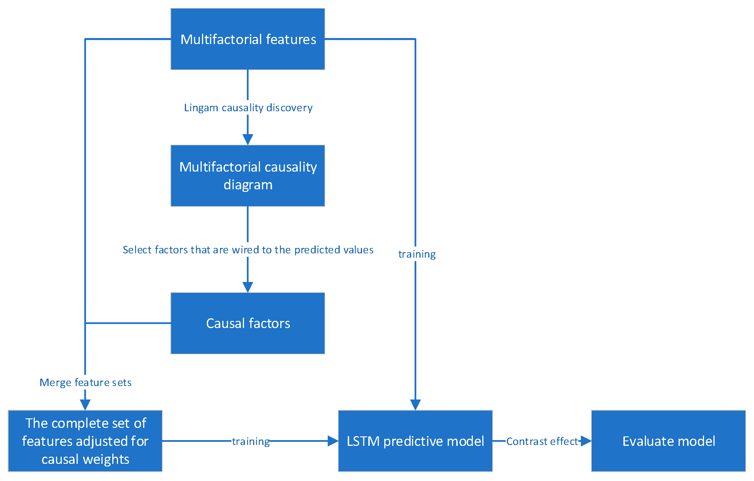
We propose a stock prediction method called LWA-LSTM based on the structural causal model. This approach begins by using a causal discovery algorithm to identify features that have a causal relationship with the predicted values within the feature set. Subsequently, these identified features are subjected to feature weight adjustment to enhance their importance within the entire feature set. Finally, the adjusted feature set is fed into a neural network for prediction. The flowchart of this method is shown in Figure 1.

Figure 1. LWA-LSTM model flowchart.

3.1. Multifactorial Forecasting

The daily real-time trading in the stock market generates a large amount of data for analysis. Various types of trading data that reflect changes in stock prices are suitable for stock price prediction, making them the focus of research. Traditional stock prediction methods often rely on single features such as opening and closing prices for forecasts. However, due to the limited number of features, these models struggle to capture the patterns of stock price fluctuations, resulting in limited predictive accuracy. A multifactor model utilizes multiple relevant features, which can improve the accuracy and robustness of stock prediction while enhancing the model’s interpretability. Therefore, we have chosen to use a multifactor model for stock forecasting.

Factors in addition to common ones such as the highest price, lowest price, and trading volume also include some manually constructed composite technical indicators. They can be divided into the following categories: scale-related features, valuation-related features, trading-related features, and price-related features. When selecting features, several factors need to be considered: firstly, the selected features should be representative and able to reflect the stock’s trading situation and changing trends; secondly, the selected features should have a strong causal relationship with the predicted value, and for predicting stock prices, they should possess greater stability and interpretability. Based on these requirements, we have selected 33 initial features for the model, which include price-related features, trading-related features, and others, as shown in Table 1.

Table 1. Complete set of multifactorial features.

Number	Factor	Number	Factor	Number	Factor
X1	next_close	X12	open_qfq	X23	macd
X2	open	X13	close_hfq	X24	kdj_k
X3	high	X14	close_qfq	X25	kdj_d
X4	low	X15	high_hfq	X26	kdj_j
X5	pre_close	X16	high_qfq	X27	rsi_6
X6	change	X17	low_hfq	X28	rsi_12
X7	pct_change	X18	low_qfq	X29	rsi_24
X8	vol	X19	pre_close_hfq	X30	boll_upper
X9	amount	X20	pre_close_qfq	X31	boll_mid
X10	adj_factor	X21	macd_dif	X32	boll_lower
X11	open_hfq	X22	macd_dea	X33	cci

3.2. LiNGAM Algorithm and Causal Weight Adjustment

Currently, the mainstream causal discovery algorithms can be classified into three main types: constraint-based methods, structure-based causal model methods, and hybrid methods. Constraint-based methods remove redundant edges in the causal graph by conducting independence tests on variables. Structure-based causal model methods start from the causal mechanisms generated by data and construct functions to determine the causal relationships between variables, thereby identifying the direction of causality. Hybrid methods combine both approaches, aiming to achieve both the high-dimensional scalability of constraint-based methods and the strong causal discovery capability of structure-based causal model methods.

Constraint-based methods often have drawbacks such as misidentification and high time complexity. Additionally, these methods are unable to learn all edges in a causal network graph; they can only obtain a directed acyclic graph comprising a set of Markov equivalent classes. On the other hand, structure-based causal modeling methods overcome these limitations by studying the distribution properties of data to discover causal relationships. However, research on hybrid approaches is still in its early stages and faces challenges like insufficient theoretical analysis. Therefore, we have chosen to study the LiNGAM algorithm, which is based on structure-based causal modeling.

LiNGAM, short for Linear Non-Gaussian Acyclic Model, was proposed by Shimizu et al. It is a variation of structural equation models and Bayesian networks. The model requires that the causal structure of the variables satisfies three conditions: first, the directed graph formed by all the variables must be acyclic; second, the model must be linear, with the target variable being a linear sum of its corresponding cause variables; third, the noise variables follow non-Gaussian distributions with nonzero variances and are mutually independent.

The variables in the LiNGAM model are generated in a causal order, so after the variables are arranged in a causal order, the variable located in the back cannot be the dependent variable of the preceding variable. In practice, the arrangement of the observed variables is random, as opposed to the causal order. We write the variables as {$v_1$, $v_2$, …, $v_n$}, denoting the causal order as $k \left(i\right)$,$i\in [1, n]. \left(i\right) \in [1, n]$ represents the position of the i-th variable in the causal order of the observation sequence, then the generation process of the variable can be described as:

$$v_i={\sum }_{k\left(j\right)<k\left(i\right)}{b}_{ij}{v}_j+n_i i,j\in [1,n]$$

(1)

In the formula, $n_i$ represents the noise terms that obey the non-Gaussian distribution, and the noise terms are independent of each other in pairs; if $b_{ij}$ is not 0, there is an edge with $v_j$ pointing to $v_i$.

Under the linear non-Gaussian acyclic conditions described above, the LiNGAM model is expressed as a matrix:

$$V=BV+n$$

(2)

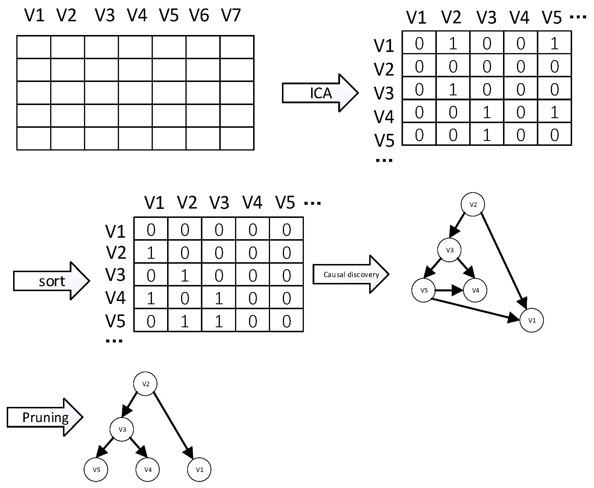
$V$ is a p-dimensional random vector, $B$ is a $p\times p$ adjacency matrix, and n is a p-dimensional non-Gaussian random noise variable. Under the assumption of a cycle-free graph, there exists a permutation matrix $P\in R^{m\times m}$ such that $B^{\prime }=PB{P}^T$ is a strictly lower triangular matrix with all diagonal elements equal to 0. This solving method is proposed based on the Independent Component Analysis (ICA) algorithm. The algorithm first obtains the limit matrix $W$ in the connection matrix $Y=WV$ from the observation data through ICA, where $Y$ is the vector containing independent components. As you can see, W has a derivation relationship with $(I-B)$. Then, combined with the characteristics of $B^{\prime }$ as a strictly lower triangular matrix, the causal order can be obtained from $W$ by using methods such as row and column permutation. Finally, after a pruning algorithm, we obtain the final cause-and-effect diagram. The basic flow is shown in Figure 2.

Figure 2. LiNGAM algorithm flowchart.

In our algorithm, we first use the daily data of the features and the closing price of the next day as variables. We apply the LiNGAM algorithm to determine the causal ordering of the variables, obtain the causal matrix, and draw a causal graph. Then, we observe the factors in the causal graph that have a causal relationship with the next day’s closing price. We select these feature factors and add them to the original feature set by duplicating a column. This increases the weight of causal feature factors in the feature set.

3.3. LSTM Algorithm

Due to the good performance of LSTM in time series data prediction, our approach selects the LSTM algorithm for stock price prediction.

The specific structure of the LSTM unit is as follows:

$$f_t=sigm\left(w_{fx}{x}_t+w_{th}{h}_{t-1}+b_f\right)$$

(3)

$$i_t=sigm\left(w_{ix}{x}_t+w_{th}{h}_{t-1}+b_i\right)$$

(4)

$$g_t=tanh\left(w_{gx}{x}_t+w_{gh}{h}_{t-1}+b_g\right)$$

(5)

$$c_t=f_t\times c_{t-1}+i_t\times g_t$$

(6)

$$o_t=sigm\left(w_{ox}{x}_t+w_{oh}{h}_{t-1}+b_o\right)$$

(7)

Among them, $f_t$ stands for the door of forgetting, which determines how much information from the upper layer will be recorded. $i_t$ represents an input gate that determines how much input information will be used. $g_t$ represents a source of alternative information, ready to update new cell status $c_t$. The final output $h_t$ is determined by the current cell state $c_t$ and the intermediate output $o_t$ and entered into the LSTM unit at the next moment. LSTM realizes the long-term transmission of information by building input, forget, and output gates, ensuring that the previous information can always participate in network training.

4. Experiment

In order to verify the effectiveness of the algorithm, we select the actual trading data of the Chinese stock market for training and predicting future stock prices, and the experimental results prove that the algorithm can better reduce the prediction error and improve the accuracy of stock prediction.

4.1. Data Sources and Preprocessing

All stock data are from the Tushare data interface package in Python. We have selected 33 factors, including opening price, trading volume, trading value, and adjustment factors, as features. The full sample period is from 20 May 2019 to 24 May 2022 and the test set selects the last 20% of the total sample set. In total, there are 733 days of data and 137 days of test sets.

Ping An Bank (000001.SZ), formerly known as Shenzhen Development Bank, is the first nationwide joint-stock commercial bank in mainland China to be publicly listed. We believe that Ping An Bank has good representativeness for the Shenzhen stock market, so we chose to conduct our experiment using it. Some of the data for it are presented in Table 2. There are various types of stocks in the stock market, and in order to ensure that the prediction errors are not caused by differences in stock types, we selected four banking stocks listed on the Shenzhen Stock Exchange: Jiangyin Bank (002807.SZ), Zhengzhou Bank (002936.SZ), and Qingdao Bank (002948.SZ) as data sources.

Table 2. Ping An Bank partial factor data graph.

Trade_Date	Close	Open	High	Low	Pre_Close	…	Boll_Mid	Boll_Lower	cci
20190520	12.38	12.35	12.54	12.25	12.44	…	12.62	11.05	−75.58
20190521	12.56	12.4	12.73	12.36	12.38	…	12.53	11.00	−45.01
20190522	12.4	12.57	12.57	12.32	12.56	…	12.42	11.01	−60.71
20190523	12.29	12.24	12.42	12.14	12.4	…	12.33	10.96	−99.07
⋮	⋮	⋮	⋮	⋮	⋮	⋮	⋮	⋮	⋮
20220523	14.83	15.07	15.07	14.76	15.02	…	14.70	13.76	35.00
20220524	14.4	14.87	14.87	14.4	14.83	…	14.63	13.74	−50.46
20220525	14.39	14.43	14.49	14.3	14.4	…	14.55	13.80	110.45

Since variables in the raw data may have different scales, we first use the fit_transform method to normalize the train data, then use the transform method on the test set. This transforms the variance to 1 and the mean to 0.

4.2. Causality Discovery

We used the LiNGAM algorithm from the causal-learn library in Python to discover causal relationships between variables. The lower limit was set to 0.9, indicating that only causal relationships with weights greater than 0.9 are displayed in the causal graph.

Due to the large number of characteristic values and the complexity of the connection between the characteristic factors, the Bank of Qingdao (002948.SZ) causal discovery is taken as an illustrative example in Figure 3.

Figure 3. Thirty-three-factor causal discovery diagram of the Bank of Qingdao.

Among them, X1 represents the closing price of the next day. From the above chart, it can be observed that the lowest price (low) has a causal relationship with the closing price. By observing the causal relationships between the remaining stocks and the closing price, the characteristic factors that have a causal relationship with the closing price are shown in Table 3: for Ping An Bank, the lowest price (low) and the closing price before adjustment (close_qfq) have a causal relationship; for Jiangyin Bank, the lowest price (low) and the trading volume (amount) have a causal relationship with X1; for Zhengzhou Bank, the lowest price (low), highest price (high), and opening price (open) have a causal relationship with X1; for Qingdao Bank, the lowest price (low) has a causal relationship with X1.

Table 3. Characteristic values in the four stocks that have a causal relationship with the closing price X1.

Stock	Features that Have a Causal Relationship with X1
000001.SZ	low, close_qfq
002807.SZ	low, amount
002936.SZ	low, high, open
002948.SZ	low

4.3. Model Building and Parameter Setting

The experimental model in this paper is built and run under the TensorFlow framework of Python 3.10, using the sequential model in Keras in TensorFlow and combining two layers of LSTM and a layer of Dense to complete the stock prediction. Above the model parameters, the number of neurons in the first layer of LSTM is 80, and the number of neurons in the second layer is 100. Optimizing parameters in 200 epochs using the Adam optimizer with a learning rate of 0.001 and a batch size batch_size of 128, the experiment uses a 10-day time step as a sliding time window. The model takes 1 day as the forecast time step, which means that we will use the stock characteristics data of the previous 10 days to predict the closing price of the stock on the eleventh day.

4.4. Evaluation Indicators

Since our job is to predict stock prices, which is a regression problem, some evaluation indicators can be used to evaluate how well our predictions work. In this paper, three evaluation indicators, mean squared error (MSE), root mean square error (RMSE), and mean absolute error (MAE), are used to evaluate the matching degree between the predicted value and true value and quantify the predictive performance of the model. The formulas for the three evaluation indicators are as follows:

$$\mathrm{M}\mathrm{S}\mathrm{E}=\frac{1}{n}\sum _{i=1}^n{\left(y_i-\widehat{y_i}\right)}^2$$

(8)

$$\mathrm{R}\mathrm{M}\mathrm{S}\mathrm{E}=\sqrt{\frac{1}{n}\sum _{i=1}^n{\left(y_i-\widehat{y_i}\right)}^2}$$

(9)

$$\mathrm{M}\mathrm{A}\mathrm{E}=\frac{1}{n}\sum _{i=1}^n\left|y_i-\widehat{y_i}\right|$$

(10)

where n is the number of samples, $y_i$ is the real data, and $\widehat{y_i}$ is the fitted data. The three evaluation indicators are used to measure the deviation between the true value and the predicted value. A smaller value indicates that the predicted value is closer to the true value, indicating that the model selection and fitting are better and that the data prediction is more successful.

4.5. Experimental Results and Analysis

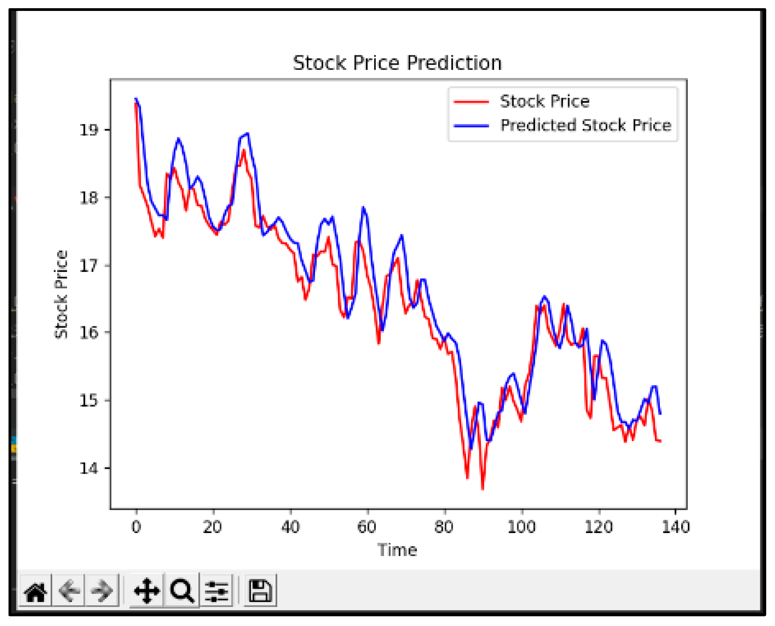
Figure 4 shows the stock price prediction graph obtained by our algorithm with 000001.SZ as an example. Table 4, Table 5 and Table 6 present the comparative results between our approach, the original LSTM model, and the LSTM model after eliminating causal feature factors. The results indicate that our algorithm outperforms in terms of all evaluation metrics for the four stocks. Particularly, Ping An Bank’s mean square error has decreased by 39.24%, achieving excellent performance.

Figure 4. Stock price prediction chart of 000001.SZ using the LWA-LSTM algorithm.

Table 4. MSE of predicted values under different causal weights.

Stock	LSTM	Remove Causal Factors	LWA-LSTM
000001.SZ	0.195848	0.230194	0.192025
002807.SZ	0.007361	0.007476	0.006347
002936.SZ	0.033469	0.027553	0.028261
002948.SZ	0.076080	0.090381	0.046225

Table 5. RMSE of predicted values under different causal weights.

Stock	LSTM	Remove Causal Factors	LWA-LSTM
000001.SZ	0.442547	0.479785	0.438206
002807.SZ	0.085796	0.086466	0.079671
002936.SZ	0.182945	0.165992	0.168110
002948.SZ	0.275827	0.300634	0.215000

Table 6. MAE of predicted values under different causal weights.

Stock	LSTM	Remove Causal Factors	LWA-LSTM
000001.SZ	0.348708	0.377324	0.352999
002807.SZ	0.060039	0.056817	0.055776
002936.SZ	0.133097	0.138641	0.119297
002948.SZ	0.159176	0.175881	0.150178

The causal feature factors selected for the experiment, represented by variables pointing to the closing price, are all dependent variables that predict the target variable, which is the closing price. Adding these feature values as an additional column to the complete set of features implies increasing the initial weights of features with causal relationships when inputting them into the neural network. After removing features with causal relationships, the predictive performance of three out of four stocks declined, demonstrating the importance of these variables in predicting the closing price. Following the implementation of the new algorithm, the prediction errors of all four stocks decreased, with the smallest prediction error observed among the three stocks. In 002948.SZ stock, the MSE error using our algorithm even dropped by 39%, further validating the effectiveness of our algorithm.

In previous research, it was widely recognized that features such as the lowest price and highest price have a positive impact on predictive effectiveness. However, there has not been any study analyzing whether this effect is based on correlation or causation. Our research demonstrates that there is a causal relationship between these feature values and the closing price. Additionally, we also provide evidence that boosting the weights of these causal features effectively enhances predictive effectiveness.

5. Summary and Outlook

In this paper, the features found with the LiNGAM algorithm are used for stock price prediction after weight adjustment. In order to make causal features play a more important role in stock price prediction, a new method is proposed in this paper, which combines the LiNGAM algorithm, feature weight adjustment, and LSTM algorithm. In this algorithm, we only select the features that point to the predicted objective in the causal graph to adjust their weights, which increases the interpretability of the method. We conducted experiments on real stock data, and the results show that our method can effectively improve prediction accuracy.

Mining the causal relationship between data to make predictions and adjust the weights of factors is a very promising research direction in the future, meeting various challenges. On the basis of this paper, future research directions can be: (1) Combining causality discovery with more advanced models such as GRU and transformers. (2) Mining the adjustment rules of feature weights to enhance the method’s generality in predicting different stocks.