Service Recommendation of Industrial Software Components Based on Explicit and Implicit Higher-Order Feature Interactions and Attentional Factorization Machines

Abstract

In the context of the rapid advancement of the Industrial Internet and Urban Internet, a crucial trend is emerging in the realization of unified, service-oriented, and componentized encapsulation of IT and OT heterogeneous entities underpinned by a service-oriented architecture. This is pivotal for achieving componentized construction and development of extensive industrial software systems. In addressing the diverse demands of application tasks, the efficient and precise recommendation of service components has emerged as a pivotal concern. Existing recommendation models either focus solely on low-order interactions or emphasize high-order interactions, disregarding the distinction between implicit and explicit aspects within high-order interactions as well as the integration of high-order and low-order interactions. This oversight leads to subpar accuracy in recommendations. Real-world data exhibit intricate structures and nonlinearity. In practical applications, different interaction components exhibit varying predictive capabilities. Therefore, in this paper we propose an EIAFM model that fuses explicit and implicit higher-order feature interactions and introduce an attention mechanism to identify which low-level feature interactions contribute more significantly to the prediction results. This approach leads to increased interpretability, combining both generalization and memory capabilities. Through comprehensive experiments on authentic datasets that align with the characteristics of the Service Recommendation of Industrial Software Components problem, we demonstrate that the EIAFM model excels compared to other cutting-edge models in terms of recommendation effectiveness, with the evaluation metrics for the AUC and log-loss reaching values of 0.9281 and 0.3476, respectively.

1. Introduction

With Industry 4.0 marked by the full use of industrial Internet of Things, the industrial system architecture has evolved from the previous centralized model to a collaborative cloud- and edge-based distributed system architecture [1]. Consequently, new industrial software has emerged to address the challenges posed by complex industrial application scenarios [2], with a focus on achieving interoperability and reusability. The service-oriented architecture (SOA) system, known for its flexibility, composability, and independence, has been recognized as the optimal solution for this scenario [3]. Therefore, the development of industrial software systems in IoT adopts a service-oriented approach, encapsulating each hardware and algorithm-related functional block into a service component, thereby enabling interoperability and facilitating reusability. This concept of service-oriented componentization represents the future direction of low-code platforms, and serves as a vital theoretical tool for digital transformation in the industrial field [4].

As mentioned earlier, industrial software service components encapsulate hardware functions to provide a flexible and efficient way to implement solutions for industrial tasks. For example, in traditional manufacturing industry, robot arm service components, sensor service components, etc., can be selected for different task requirements in shop floor production scenarios to coordinate the flow of production tasks. In addition, service components avoid the problem of repeated development, effectively reducing development costs, as the same service component can be applied to different scenarios and tasks according to the requirements. Users do not need to have advanced programming knowledge, only to understand the combination of component functions according to the task scenario. The above advantages make service components a powerful tool to meet different task requirements. In this context, the number of industrial software service components is rapidly increasing, and implementing service component recommendations for different tasks to improve component utilization and reduce the development cost of manual selection is becoming a key technical issue.

The recommendation domain has long been at the forefront of technological advancement and innovation. Numerous methods have been introduced to enhance the precision of service recommendations. In previous research, these have been broadly classified into two categories, namely, traditional recommendation models and deep learning recommendation models. Traditional recommendation models such as Collaborative Filtering (CF) [5,6,7], Matrix Factorization (MF) [8,9,10], Logistic Regression (LR) [11], and Factorization Machines (FM) [12,13,14] rely on the advantages of strong interpretation, fast training, and low hardware requirements for easy deployment; they are used in a large number of practical scenarios, and form the basis of deep learning models. However, traditional models may not possess strong generalization capabilities, rely more on manual preprocessing, and do not take into account the higher-order relationships between features. To address these shortcomings, deep learning recommendation models have been proposed in the recommendation domain, such as the AutoRec system [15] proposed by the Australian National University. AutoRec integrates AutoEncoder principles with Collaborative Filtering, presenting a neural network recommendation model featuring a single hidden layer. However, its simple structure suffers from a certain lack of expressive power. Google proposed the Wide&deep model [16] in 2016, combines the memory Capability of traditional low-order feature interaction with the generalization capability of deep learning model. This initiated the idea of fusing different network structures. DeepFM [17] is an integration of the FM model structure with the Wide&deep model; however, it ignores either the explicit and implicit feature interactions or does not closely combine the higher-order and lower-order feature interactions, resulting in missing information and making the recommendation results less accurate. In the real world, data are nonlinear and have a complex structure; indeed, different interaction components have varying predictive capabilities.

To address these issues, in this paper we propose a new model named EIAFM that incorporates explicit and implicit higher-order feature interaction components to better capture the higher-order features of complex nonlinear structures. Additionally, we introduce an attention mechanism to measure the differential importance of lower-order feature interactions [18]. The probability that a task target in industry invokes an industrial software service component is the target predicted by our model. On a real-world dataset that meets the problem description definition, our comprehensive experiments show that EIAFM outperforms several cutting-edge models in terms of recommendation. In summary, this paper makes the following contributions:

• The innovation of the EIAFM model lies in its integration of explicit and implicit higher-order feature interactions to accurately capture valuable information from complex data. Furthermore, the introduction of an attention mechanism enables precise measurement of the varying importance within feature interactions, endowing the model with both low-level memory capability and high-level generalization ability.
• An industrial software service component recommendation framework based on EIAFM is proposed, which is mainly applicable to typical industrial collaborative manufacturing systems; its application can obtain better service component recommendation results.
• Comprehensive experiments are conducted using a real dataset that fits the description of the Service Recommendation of Industrial Software Components problem; the experimental outcomes demonstrate the notable superiority of the proposed EIAFM model over several mainstream recommendation approaches.

The rest of this paper is structured as follows: Section 2 introduces related papers in the field of service recommendation; Section 3 develops a recommendation architecture for industrial collaborative manufacturing systems based on EIAFM; Section 4 proposes the EIAFM model, which contains the problem description of industrial software service component recommendation, existing mainstream FM-based service recommendation models (FM, AFM, XDeepFM), and the relationship between EIAFM and the above models; Section 5 conducts an extensive experimental evaluation using a real dataset that fits the problem definition of industrial software service component recommendation; and finally, Section 6 summarizes the contributions of this paper while offering a glimpse into prospective future research directions.

2. Related Work

The research on service recommendation models is mainly divided into traditional recommendation models and deep learning recommendation models, although there is a close relationship between the two, and the evolution of the FM model reflects the innovation of different features across methods. This paper primarily addresses lower-order feature interactions and higher-order feature interactions. In lower-order feature interactions, the relationships between features are linear and the influence of each feature on others is independent, with no complex interactions. In higher-order feature interactions there may be nonlinear relationships between features, feature combinations, cross-features, etc. In such cases the relationships between features are more complex, requiring higher-order models for modeling.

2.1. Traditional Recommendation Models

Despite the current popularity of deep learning, traditional models can offer significant advantages, including strong interpretability, low hardware requirements, quick deployment, and training capabilities. These advantages make them particularly valuable in industry applications where effectiveness is a priority. Collaborative filtering, for instance, has gained substantial attention since Amazon’s publication on the topic in 2003 due to its strong interpretability. However, it lacks the ability to generalize well, meaning that it cannot efficiently calculate the similarity between items based on their shared characteristics, leading to challenges when dealing with vector sparsity issues [19,20,21]. To address this problem, matrix decomposition-based recommendation algorithms have been proposed, which strengthen the model’s ability to handle sparse matrices. Compared with collaborative filtering, matrix decomposition has the following advantages: (1) strong generalization ability, which can solve the problem of data sparsity to a certain extent; (2) low space complexity, without the need to store the collaborative filtering service larger dimensional similarity matrices; and (3) strong scalability and flexibility [22,23,24]. Matrix decomposition has drawbacks, however; as with collaborative filtering, matrix decomposition cannot make effective recommendations when it lacks historical information. In order to solve this problem, logistic regression models and the subsequent development of models such as factor decomposition machines with different feature fusion capabilities have become more widely used in the recommendation field.

Logistic regression converts the recommendation problem into a click-through rate (CTR) prediction problem [25]. Insufficient expressive power of logistic regression methods result in an inability to perform higher-order operations of feature crossover, leading to loss of information. In order to solve this problem, higher-dimensional complex models, such as factor decomposition machines, have been derived. For the feature crossing problem, engineers often use a manual combination of features and then filter features through various analysis means; however, this method is too dependent on manual experience. The POLY2 model [26] seeks to address this by crossing all features two by two, and does not assign weights to all combinations, which solves the feature combination problem to an extent by violent combination. However, violent combination makes the feature vectors even sparser when dealing with sparse vectors, which leads to a lack of effective data for training and inability to converge. In order to overcome the defects of the POLY2 model, Rendle proposed the FM model, which assigns a hidden vector to each feature and uses the inner product of the corresponding hidden vectors as the weight when two features are intersected, thereby solving the problem of data sparsity and reducing the parameter size of the model by introducing hidden vectors. The FM-based FFM model [27], on the other hand, introduces the concept of feature domain perception, which makes the model more expressive.

2.2. Deep Learning Recommendation Models

In contrast with conventional recommendation models, deep learning recommendation models can extract hidden information from data, and have stronger expression ability. AutoRec combines a self-encoder with collaborative filtering, and uses a single hidden layer neural network model. The idea revolves around employing the co-occurrence matrix within collaborative filtering for the purpose of vector self-coding, then using the results of the self-coding to produce a predicted score for service recommendation. The AutoRec model’s architecture is quite straightforward, though it lacks expression ability. Microsoft proposed the Deep Crossing model [28], a complete solution for feature engineering from sparse vectors to dense vectors and multi-layer neural networks for optimization of fitting and other deep learning applications in the field of recommendation. This model uses embedding coupled with a multi-layer neural network structure; the original features are input into the neural network structure through embedding to carry out model training, which can be adjusted by changing the depth of the network when carrying out feature crossover. Similarly, the main contribution of the PNN model proposed by the Shanghai Jiao Tong University [29] lies in the feature crossover part of the product. The feature crossover part is divided into the outer product and the inner product. The structural characteristics of this model emphasize the crossover of the different features, making the model good for capturing the feature crossover information; however, the PNN model crosses all the features without any discrimination, which ignores the valuable information of the original features.

The Wide&deep model consists of a multi-layer deep part and a single-layer wide part, providing the model with both memory and generalization capabilities while opening up the idea of feature structure fusion. The similar Deep&cross model has been proposed by researchers at Stanford University and Google [30]; it replaces the previous wide layer with a cross layer to increase the degree of feature crossover while avoiding the need for manual feature engineering based on experience.

2.3. Factorization Machine-Based Models

As deep learning advances, FM models are gradually evolving. The FNN model proposed by the University of London [31] mainly solves the problem of training convergence with embedding, for which it uses the hidden vectors of individual feature vectors trained by the FM model as the initialization parameters of the embedding layer. It is understood as the initialization of the network parameters with the addition of a priori information, accelerating the neural network’s convergence. The structure is simple, and there is no separate feature cross layer. Harbin University and Huawei researchers proposed DeepFM optimized for the Wide&deep model to replace the original wide layer with the FM model. The resulting model has automatic feature combination capability. Deep&cross is different in its use of multi-layer cross-network feature combination, while DeepFM uses FM for combination. xDeepFM [32], on the other hand, improves on CrossNet by proposing a compressed interaction network, which avoids the situation in which the output of each hidden layer and the initial vectors are scalar multiples by making the interaction of the vectors bit-level. However, it ignores the combination of lower-order and higher-order interactions. The AFM [33] model proposed by Zhejiang University, on the other hand, introduces an attention mechanism to measure valuable information; however, it is limited to low-order feature interactions and ignores the importance of high-order interactions. The current deep learning technique based on the FM model is a more advanced recommendation model, which has the advantage of modeling the complex relationship hidden in the higher-order and lower-order interactions [34,35].

In summary, current recommendation models either have only low-order interaction modeling, neglecting the nonlinearity and intricate structure inherent in actual data, or focus only on high-order feature interactions while ignoring the mutual complementarity of explicit and implicit interactions, making them unable to better integrate low-order and high-order feature interactions. In real complex application scenarios, different interaction components exhibit different predictive capabilities; thus, a new model is needed to fit the application scenario in which a model captures high-order explicit and implicit interactions and infers which low-level feature interactions contribute more significantly to the predictions. On the other hand, for the recommendation problem of service components in industrial software it is necessary to improve the existing deep learning models and build an efficient recommendation architectures in accordance with the actual application to improve the recommendation accuracy and component utilization, which is the research motivation of this paper.

3. Recommended Architecture for Industrial Software Service Components

The following describes the proposed framework for industrial software service component recommendation, as shown in Figure 1. The framework applies to the scenario of a typical industrial collaborative manufacturing system based on the proposed explicit and implicit higher-order feature interactions and attentional factorization machine model.

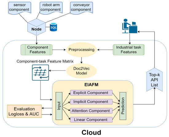
Figure 1. Industrial software service component recommendation framework based on EIAFM mode.

In this scenario, end-node devices are encapsulated in a microservice style to form service components and invoked through APIs such as sensor components, robotic arm components, conveyor components, etc. Features such as component descriptive information, prevalence, and categories are stored by the edge nodes, which transmit the component feature information to the cloud, while the staff transmit features such as descriptive information and categories of the industrial tasks to the cloud. The cloud repository not only stores the above two kinds of feature information, it stores the combination relationship between historical industrial tasks and service components. The description information of service components and industrial tasks in the cloud repository is preprocessed, usually in the steps of stemming, normalization, tagging, and stop-word deletion, then the processed results are used as inputs to the Doc2Vec [36] model. It is precisely because Doc2Vec is designed to learn embeddings for entire documents or paragraphs that it is more suitable for capturing document-level semantic information, such as descriptions of industrial tasks and service components. The textual representation of the description information is transformed into a vectorial representation, based on which the similarity between the industrial task description information and the service component description information are calculated using the cosine similarity. Subsequently, additional relevant attributes, including factors such as the popularity of industrial service components, the category of industrial service components, and industrial tasks, are retrieved from the cloud industrial service database to form a feature matrix. In summary, the feature matrix consists of vector representations of relevant feature attributes of service components and industrial tasks, such as categories, description statements, similarities, etc. This matrix is then processed and serves as the training data for the EIAFM model.

The EIAFM model has five components: a prediction component, implicit component, attention component, explicit component, and linear component. The linear component discerns the direct relationship among the input and the goal, the implicit component is used to capture the information about the implicit higher order feature intersections, the explicit component is used to capture the information about the explicit higher-order feature intersections, the attention component is used to quantify the contributions of different second-order feature interactions to the prediction results, and the prediction component finally sums the initial four outputs and estimates the recommendation probability using a sigmoid function. The model’s performance is evaluated using the AUC and log-loss metrics during the training process. The reason for using the AUC value is because it can robustly measure the model’s ability to identify positive and negative samples under different threshold settings. When using the EIAFM model trained with data on historical industrial tasks and service component combination relationships, the framework recommends the top-k ranked industrial based on staff members’ descriptions of the industrial task requirements and software service components with the highest probability.

4. Combination of Explicit and Implicit Higher-Order Feature Interaction and Attentional Factorization Machines

In this segment, we first outline the problem definition for the recommendation of industrial software service components related to industrial tasks. Then, the structure and formulas of the current FM-based recommendation models (basicFM, AFM, XDeepFM) are presented as prior knowledge, followed by outlining the architecture and mathematical equations employed in our EIAFM model. Finally, the relationship between the EIAFM and current FM-based recommendation models is compared, demonstrating the theoretical advantages of the proposed model.

4.1. Problem Definition

In common industrial scenarios, for an industrial task set $M=\left\{m_1,m_2,m_3,\dots \right\}$ and component set $C=\left\{c_1,c_2,c_3,\dots \right\}$, the expression of the model’s prediction function takes the form

$$y:M\times C\to R.$$

(1)

In the above formula, $y(m,c)$ is the anticipated score, which represents the industrial task m on the service component c. In the recommendation scenario of the industrial software service component, the recommendation probability is predicted using the description information of the industrial task and the industrial software service component, the similarity between the industrial task and the industrial software service component, the popularity of the industrial software service component, and the category information of the industrial task and the industrial software service component, which are used as the input feature vectors of the model. Thus, for the recommendation problem in (1), it can be represented by the formula below:

$$y:DC\times DM\times SIM\times POC\times CC\times CM\to S$$

(2)

The above formula takes six main aspects of features as inputs: $DC$ denotes the descriptive information of the service component, $DM$ denotes the descriptive information of the industrial task, $SIM$ denotes the similarity between the service component and the industrial task, $POC$ denotes the prevalence of the service component, $CC$ denotes the class of the service component, $CM$ denotes the class of the industrial task, and S is the final prediction score. The service component recommendation in the thesis is related to the prediction of the probability of the industrial task invoking the service component.

4.2. FM-Based Models for Service Recommendation

4.2.1. Introducing Hidden Vectors

A factorization machine (FM) is based on logistic regression. By adding the second-order feature crossover part, introducing the concept of hidden vectors for each feature, and using the inner product of the hidden vectors as the weight of each combination of features, the introduction of hidden vectors solves the problem of data sparsity and provides second-order crossover ability. This enhances the model’s expression capability compared to logistic regression; however, because of the combinatorial complexity, extending the FM model to higher-order feature interactions presents challenges. The FM is defined as follows:

$${\widehat{y}}_{FM}\left(x\right)=w_0+\sum _{i=1}^n{w}_i{x}_i+\sum _{i=1}^n\sum _{j=i+1}^n⟨v_i,v_j⟩x_i{x}_j.$$

(3)

With the parameters $w_0\in \mathbb{R}$, $W\in {\mathbb{R}}^n$, and $V\in {\mathbb{R}}^{n\times k}$, where $w_0\in \mathbb{R}$ represents the global bias term, $w_i$ signifies the strength of the impact that the ith feature has on the outcome variable, $⟨.,.⟩$ denotes two vectors making up an inner product, $v_i$ is the ith row variable of V having k factors, denoted as the embedding vector of the ith feature, i.e., the hidden vector, and $k\in {\mathbb{R}}_0^{+}$ is a hyperparameter defining the dimension of the factorization.

4.2.2. Measuring Feature Importance

Because FM uses the same weight for all combined features, incorporating unnecessary feature interactions introduces noise and diminishes the predictive efficacy. Introducing an attention mechanism can help to measure the importance of different features, making the model more interpretable. The network’s input consists of an interaction vector formed by two features, and the combined information is encoded within the embedding domain; the output is the attention score corresponding to the combined features. The network responsible for attention can be characterized as follows:

$$\begin{array}{c}{a}_{ij}^{\prime }={\mathit{h}}^{T}ReLU\left(W\left(v_i\odot v_j\right)x_i{x}_j+b\right)\\ a_{ij}=\frac{exp\left(a_{ij}^{\prime }\right)}{{\sum }_{(i,j)\in {\mathbb{R}}_x}exp\left(a_{ij}^{\prime }\right)}\end{array}$$

(4)

The parameters are defined as $W\in {\mathbb{R}}^{t\times k}$, $b\in {\mathbb{R}}^t$, and $h\in {\mathbb{R}}^t$, with t signifying the dimensionality of the hidden layer within the attention network, often referred to as the attention factor. The result from the attention pooling layer is a k-dimensional vector that efficiently compresses features within the representation space through interactive operations into a single vector, uses different weights to differentiate their importance, and projects the vector onto the prediction score. The overall formulation of the introduced structure of the attention mechanism model is outlined as follows:

$$\begin{array}{cc}\hfill {\widehat{y}}_{AFM}\left(\mathit{x}\right)=& w_0+\sum _{i=1}^n{w}_i{x}_i+\hfill \\ \hfill & {\mathit{p}}^T\sum _{i=1}^n\sum _{j=i+1}^n{a}_{ij}⟨v_i\odot v_j⟩x_i{x}_j\hfill \end{array}$$

(5)

The above equation contains two parts; the first part is a linear model which weights and sums the input embedding vectors, and the second part is a nonlinear model which first performs element-wise product operation on every two input embedding vectors to obtain a new vector. These interaction vectors are then weighted, the weighted vectors are pooled by the attention scores obtained from Formula (4), and the neural weights of the prediction layer are finally weighted with p to obtain the final prediction results. The interactions of the higher-order features are not taken into account.

4.2.3. Explicit and Implicit Higher-Order Feature Interactions

DNNs are good at learning higher-order interactions between features; however, a DNN is a kind of implicit feature interaction which is learned at a bit-wise level, and its interpretability is not high. Thus, we designed a higher-order explicit cross-feature Compressed Interaction Network (CIN) and combined it with the DNN to form a combination of explicit and implicit higher-order interactions. These mainly consists of two components, namely, the CIN component and the DNN component; the computation of each layer of the CIN network based on the fixed formulas is defined as follows:

$${\mathbf{X}}_{h,\ast }^k=\sum _{i=1}^{H_{k-1}}\sum _{j=1}^m{\mathbf{W}}_{ij}^{k,h}\left({\mathbf{X}}_{i,\ast }^{k-1}\circ {\mathbf{X}}_{j,\ast }^0\right)$$

(6)

Here, ${\mathbf{X}}^0\in {\mathbb{R}}^{m\times D}$ is the input to the model, i.e., m features, the dimension of embedding is a matrix stacked in D dimensions, ${\mathbf{X}}_{i,\ast }^0=e_i$ denotes the embedding vector corresponding to the ith feature $e_i$, the superscript denotes the kth layer of the network, ${\mathbf{X}}^k\in {\mathbb{R}}^{H_k\times D}$ denotes the output matrix of the kth layer of the CIN network, D is the dimension of the embedding, $H_k$ is the number of features in the kth layer (which can be viewed as the number of neurons in that layer), ${\mathbf{X}}_{h,\ast }^k$ is the hth eigenvector of layer k, the range of values of h is $1\le \mathrm{h}\le H_k$, ${\mathbf{W}}^{k,h}\in {\mathbb{R}}^{H_{k-1}\times m}$ is the parameter matrix of the hth feature, and ∘ means the Hadamard product $<a_1,a_2,a_3>\circ <b_1,b_2,b_3>=<a_1{b}_1,a_2{b}_2,a_3{b}_3>$. The formula shows that ${\mathbf{X}}^k$ is the result of a calculation performed by ${\mathbf{X}}^{k-1}$ and ${\mathbf{X}}^0$, which for the ith feature vector is sequentially multiplied with the other m feature vectors in a Hadamard product operation by the weights of the corresponding positions and summed to obtain a D-dimensional vector, which is ${\mathbf{X}}_{h,\ast }^k$. Thus, each feature of the matrix is output one by one according to the varying neuron counts across layers following the same steps. Explicit higher-order interactions of features are of vector-size level, which is easily achieved through the CIN network. For the analysis of the above equation, each output feature vector at layer k combines the information from the explicit higher-order interactions of each embedding vector in the input, then the matrix of $H_k\times D$ is summed along the D-dimension to obtain the vector of $H_k$ with the following formula:

$$p_i^k=\sum _{j=1}^D{\mathbf{X}}_{i,j}^k$$

(7)

where $i\in \left[1,H_k\right]$, the pooling vector is ${\mathbf{p}}^k=\left[p_1^k,p_2^k,\dots ,p_{H_k}^k\right]$, the length of the kth hidden layer is $H_k$, and the pooled vectors from each layer are spliced to obtain the output of the final CIN: ${\mathbf{p}}^{+}=\left[{\mathbf{p}}^1,{\mathbf{p}}^2,\dots ,{\mathbf{p}}^T\right]\in {\mathbb{R}}^{{\sum }_{i=1}^T{H}_i}$.

As mentioned earlier, xDeepFM complements both CIN and DNN, including both explicit and implicit higher-order interactions while adding linear components; the final model output equation is

$$\widehat{y}=sigmoid\left({\mathbf{w}}_{\mathrm{linear}}^T\mathbf{a}+{\mathbf{w}}_{dnn}^T{\mathbf{x}}_{dnn}^k+{\mathbf{w}}_{\mathrm{cin}}^T{\mathbf{p}}^{+}+b\right),$$

(8)

where $\mathbf{a}$ represents the original features ${\mathbf{x}}_{dnn}^k$, ${\mathbf{p}}^{+}$ denotes the respective results yielded by the DNN and CIN, respectively, and ${\mathbf{w}}_{\ast }$ and b are the learnable parameters.

4.3. Explicit and Implicit Higher-Order Feature Interactions and Attention Factorization Machine for Service Component Recommendation

In order to simultaneously learn nonlinear explicit and implicit high-order feature interactions and measure the varying importance of feature interactions, we propose a novel model structure, EIAFM, which employs a compressed interaction network to capture explicit higher-order feature interactions, a deep neural network to extract valuable information from implicit higher-order feature interactions, and attention weights to measure the contributions of cross-features to prediction results, thereby enhancing model interpretability. From a mathematical perspective, the EIAFM model formula is derived by incorporating two additional nonlinear functions onto the foundational Formula (5):

$$\begin{array}{cc}\hfill & {\widehat{y}}_{EIAFM}\left(\mathbf{x}\right)=w_0+\sum _{i=1}^n{w}_i{x}_i+g\left(\mathbf{x}\right)+f\left(\mathbf{x}\right)\hfill \\ \hfill & +{\mathbf{p}}^T\sum _{i=1}^n\sum _{j=i+1}^n{a}_{ij}⟨{\mathbf{v}}_i\odot {\mathbf{v}}_j⟩x_i{x}_j\hfill \end{array}$$

(9)

Here, the first and second terms are nonlinear components similar to the FM, the third captures the explicit higher-order component, the fourth captures the implicit higher-order component, and the fifth is the interaction of different attention scores for second-order features. In this paper, these four components are referred to as the linear component, implicit component, explicit component, and attention component. Equation (9) can be interpreted as follows:

$${\widehat{y}}_{EIAFM}\left(\mathbf{x}\right)={\widehat{y}}_{LC}\left(\mathbf{x}\right)+{\widehat{y}}_{EC}\left(\mathbf{x}\right)+{\widehat{y}}_{IC}\left(\mathbf{x}\right)+{\widehat{y}}_{AC}\left(\mathbf{x}\right)$$

(10)

$$\begin{array}{c}\hfill where\left\{\begin{array}{cc}\hfill {\widehat{y}}_{LC}\left(\mathbf{x}\right)& =w_0+\sum _{i=1}^n{w}_i{x}_i\hfill \\ \hfill {\widehat{y}}_{EC}\left(\mathbf{x}\right)& =g\left(\mathbf{x}\right)\hfill \\ \hfill {\widehat{y}}_{IC}\left(\mathbf{x}\right)& =f\left(\mathbf{x}\right)\hfill \\ \hfill {\widehat{y}}_{AC}\left(\mathbf{x}\right)& ={\mathbf{p}}^T\sum _{i=1}^n\sum _{j=i+1}^n{a}_{ij}⟨{\mathbf{v}}_i\odot {\mathbf{v}}_j⟩x_i{x}_j\hfill \end{array}\right.\end{array}$$

(11)

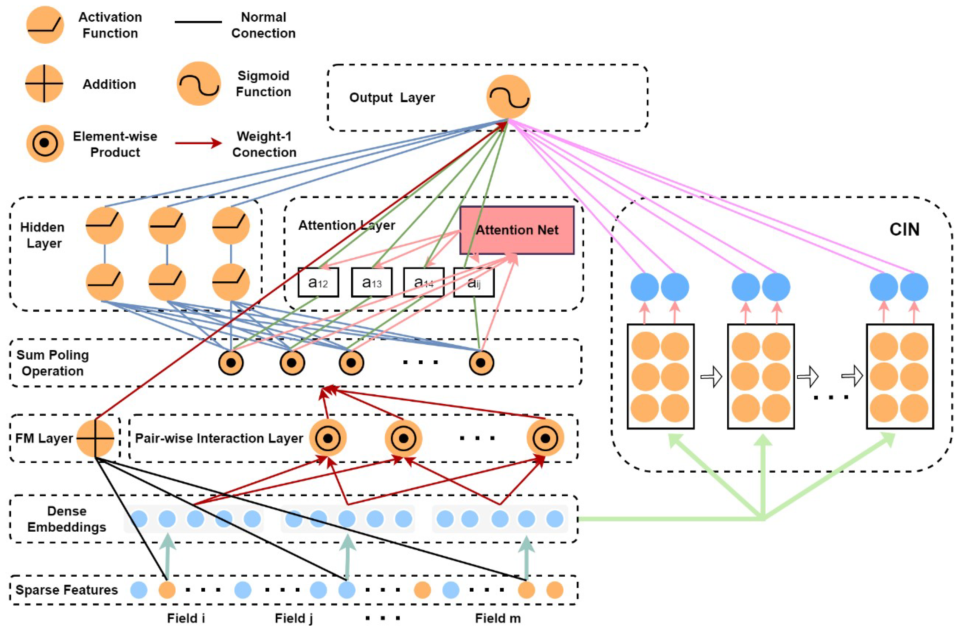
Figure 1 presents a visual depiction of the EIAFM model proposed in this article. The input and embedding layers are identical to those in the FM model, with sparse vector representations of the input features which are then mapped and embedded into dense vectors, and the model parameters of the linear components are ${\Theta }_{LC}=\left\{w_0,{\left\{w_i\right\}}_{i=1}^n\right\}$. Figure 2 shows how the embedding layer compresses the input vectors into low-dimensional dense vectors to facilitate network training, the embedding set ${\mathbf{v}}_x$ is input to the pairwise interaction layer, and a set of embedding vectors is mapped into a single vector by a pooling operation, as described by the following formula:

$$f_{PI}\left({\mathbf{v}}_x\right)=\sum _{i=1}^n\sum _{j=i+1}^n{\mathbf{v}}_i{x}_i\odot x_j{\mathbf{v}}_x$$

(12)

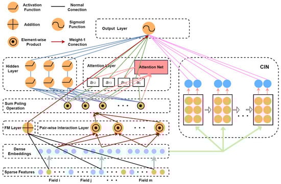
Figure 2. The network architecture of the EIAFM model.

In the model, the pair-wise interaction layer generates a k-dimensional vector to represent the second-order interaction relationships among different features in the embedding domain, conveying information about how these features influence each other. In the xDeepFM and AFM models, the input data for the attention layer and the hidden layer are not the same. The architecture of the EIAFM model is different from both in that it pools the vector outputs from the pair-wise interaction layer and utilizes the processed data as the joint input for both the attention layer and the hidden layer. This aids in the convergence of the model during training. Simultaneously, EIAFM employs sparse features as training data for the FM layer, and the output of the embedding layer serves as the input for the CIN network. Additionally, for the implicit component’s output, $Q_L$ is partially mapped to the result based on weights:

$$f\left(x\right)={\mathbf{h}}^T{Q}_L.$$

(13)

In this context, the vector $\mathbf{h}$ represents the weights associated with the implicit component prediction layer, and Formula (13) can be generalized as follows:

$$f\left(\mathbf{x}\right)={\mathbf{h}}^T{\sigma }_L\left({\mathbf{W}}_L\left(\cdots {\sigma }_1\left({\mathbf{W}}_1{f}_{PI}\left({\mathbf{v}}_x\right)+{\mathbf{b}}_1\right)\cdots \right)+{\mathbf{b}}_L\right)$$

(14)

where L represents the count of hidden layers, ${\mathbf{W}}_L$ represents the weight matrix, ${\mathbf{b}}_L$ is the bias vector, and ${\sigma }_L$ denotes the activation function for the ith layer. The parameters related to the implicit component in the model are represented by ${\Theta }_{IC}=\left\{\mathbf{h},\left\{{\mathbf{W}}_L,{\mathbf{b}}_L\right\}\right\}$, and are depicted by the blue link in Figure 2.

In the attention component, the feature interactions are subjected to an attention mechanism in which the sum of the interacting vectors is weighted. The definition of the attention network follows the same structure as that described in Formula (4). The outcome of the pooling layer, which depends on the attention mechanism, is subsequently projected to be proportional to the predicted score. It corresponds to the term identified as the fifth in Formula (9), and the attention model’s parameter set is ${\Theta }_{AC}=\left\{\mathbf{p},\mathbf{W},\mathbf{b},\mathbf{h}\right\}$.

For the explicit component, higher-order feature interactions are explicitly learned using the CIN network, which models the interactions at the vector level. The resulting dense embedding vectors are used as inputs to the CIN network; each layer of the CIN network is defined in a manner consistent with Formula (6), and the pooled vectors from each layer are concatenated to form the ultimate CIN output vector. This CIN output vector contributes to the prediction score and corresponds to the third term in Formula (9):

$${g\left(\mathbf{x}\right)=\mathbf{p}}^{+}=\left[{\mathbf{p}}^1,{\mathbf{p}}^2,\dots ,{\mathbf{p}}^T\right]\in {\mathbb{R}}^{{\sum }_{i=1}^T{H}_i}$$

(15)

where T signifies the count of hidden layers in CIN, ${\mathbf{p}}^i$ is the pooling vector of each layer, ${\mathbf{p}}^{+}$ is the final output vector of the CIN, and the model parameters of the CIN network are ${\Theta }_{EC}=\left\{{\mathbf{W}}_{cin},\mathbf{b}\right\}$. To summarize EIAFM, the overall parameters of the model are $\Theta =\left\{{\Theta }_{LC},{\left\{{\mathbf{v}}_i\right\}}_{i=1}^n,{\Theta }_{IC},{\Theta }_{AC},{\Theta }_{EC}\right\}$, which contain the embedding vector.

The problem of recommending industrial software service components can be regarded as a classification task. A sigmoid function is employed in the ultimate output transformation to $y\left(\mathbf{x}\right)=sigmoid\left({\widehat{y}}_{EIAFM}\left(\mathbf{x}\right)\right)$. In the context of regression, $y\left(\mathbf{x}\right)$ represents a real-valued variable, and we can aggregate the final results from the four components. In the case of binary classification tasks, cross-entropy commonly serves as the loss function for evaluating the predictive performance. Therefore, the loss function for EIAFM is formally expressed as Formula (16), and L2 regularization is employed within the model to avoid overfitting.

$$L(\Theta )=-\frac{1}{n}\sum _{i=1}^n\left[y^{\left(i\right)}ln\left({\widehat{y}}^{\left(i\right)}\right)+\left(1-y^{\left(i\right)}\right)ln\left(1-{\widehat{y}}^{\left(i\right)}\right)\right]$$

$$+\frac{\lambda }{2m}\sum _{j=1,{\theta }_j\in \Theta }^m{\theta }_j^2$$

(16)

Here, n is the the number of samples, $\lambda$ regulates the strength of L2 regularization, and the training of the EIAFM model involves the utilization of stochastic gradient descent.

4.4. Relationship of EIAFM to Existing FM-Based Models

The mathematical formulation of the model described in Section 4.2 and Section 4.3 can potentially encapsulate the connection between existing FM-based models and EIAFM. Table 1 compares the models from five aspects; notably, EIAFM is the only model that captures explicit and implicit higher-order interactions and the different importance of second-order feature interactions at the same time. EIAFM improves on xDeepFM and AFM while reducing the complexity of the model through the summing–pooling operation.

Table 1. Contrasting FM-Based Models.

Models	Order-One Features	Order-Two Features	Explicit High-Order Features	Implicit High-Order Features	Distinguish the Importance of Order-2 Feature Interation
basicFM	✓	✓	×	×	×
DeepFM	✓	✓	×	✓	×
AFM	✓	✓	×	×	✓
xDeepFM	✓	✓	✓	✓	×
EIAFM	✓	✓	✓	✓	✓

5. Experiments and Discussion

This section provides the experimental outcomes used to assess the proposed EIAFM model. Considering that FM-based models have been established as the most highly endorsed models in the field, we contrasted EIAFM against models containing AFM, basicFM, deepFM, and xdeepFM. In addition, we compared the outcomes of various parameters of EIAFM and studied the performance of its different components. The experimental results of EIAFM are summarized as follows. EIAFM is implemented using TensorFlow. We first describe the original dataset for the experiments, then introduce the evaluation of the indicators, and finally present the experimental findings. The experimental configurations and versions are as follows: Numpy-1.15.4, Pandas-1.1.5, Tensorflow-1.4.0, Python-3.6.13.

5.1. Dataset

Following the problem definition in Section 4.1, we chose a real-world dataset that meets the description to perform verification experiments. In order to ensure the reliability of our experimental results, we used a dataset from ProgrammableWeb [37] and divided the data into two parts: Web APIs and Mashup application tasks. In the dataset, Web APIs are single-API services which contain APIName, category, description text, port number, etc., while Mashups are a web application tasks composed of multiple Web APIs, which include MashupName, category, MemberAPIs, description text, etc. The dataset consists of 12,919 Web APIs and 6206 Mashups. This real dataset conforms to the problem definition for the recommendation scenario of industrial software service components. According to the statistics, only 940 of all API components are called by the task, or 7.28% = 940/12,919. Even though the majority of the APIs are not called, there are a total of 9297 task–API interactions. The dataset’s attributes are presented in Table 2:

Table 2. Attributes for the training dataset.

Items	Values
Quantity of Mashups	6206
Count of APIs	12,919
Invocations Quantity	9297
Count of invoked APIs	940
The quantity of APIs for each Mashup	2.08
Mean API description length	76.84
Mean Mashup description length	36.57
Proportion of Invoked APIs	7.28%

5.2. Evaluation Metrics

To assess the performance of the classification models, we utilized two distinct evaluation metrics, namely, the log-loss and AUC. The log-loss measures the discrepancy between predicted and actual sample scores, while the AUC quantifies the probability of the classifier randomly selecting positive samples ranking higher than randomly selected negative samples. A superior model will have an AUC value close to 1, implying a good separability measure. In the task scenario of this experiment, the interactions between the task and the service API were observed as positive samples, whereas unobserved interactions constituted negative samples.

5.3. Comparative Evaluation and Analysis of Performance

Taking into account the sparsity of the matrix representing Mashup tasks and API services within the dataset, along with the imbalanced distribution of positive and negative samples, we opted to utilize a subset consisting of the 100 most popular APIs and their associated Mashups (1993 in total) as the experimental data to serve as the dataset for experimentation. The length of the descriptive information of all the tasks and service APIs was short, the vector size was set to 50 in Doc2Vec modeling, and the quantity of positive samples was increased from the selected service APIs and the tasks, for a total of 2405 calls. This resulted in the acquisition of 2405 positive instances. Furthermore, to obtain a balanced dataset, 2595 instances were randomly chosen from the original dataset, where no call relations existed between industrial tasks and industrial software service components. These selected instances were included as negative samples to enhance the dataset’s balance.

The test dataset was evaluated using the AUC and log-loss as performance metrics to experimentally demonstrate the effectiveness of EIAFM, as well as to investigate the effects of the parameters and individual constituent components of EIAFM on the model. In the above experiments, all evaluation metrics were conducted using the preprocessed dataset; for greater accuracy of the experimental results, the average values of all evaluation metrics across ten rounds were used as the benchmark. The default values of the hyperparameters for EIAFM and the configuration of relevant models for comparative experiments are shown in Table 3:

Table 3. Default hyperparameter settings across all models.

Items	Values
Iteration count for the model	100
Training batch size per iteration	128
Size of the test dataset	20%
Hidden units in a two-layer configuration	(64,64)
Factor of attention	32
Units in a two-layer CIN configuration	(4,4)
Strength of L2 regularization	0.001
Rate of dropout	0.5
Value of seed	0

5.3.1. Recommended Performance Comparison

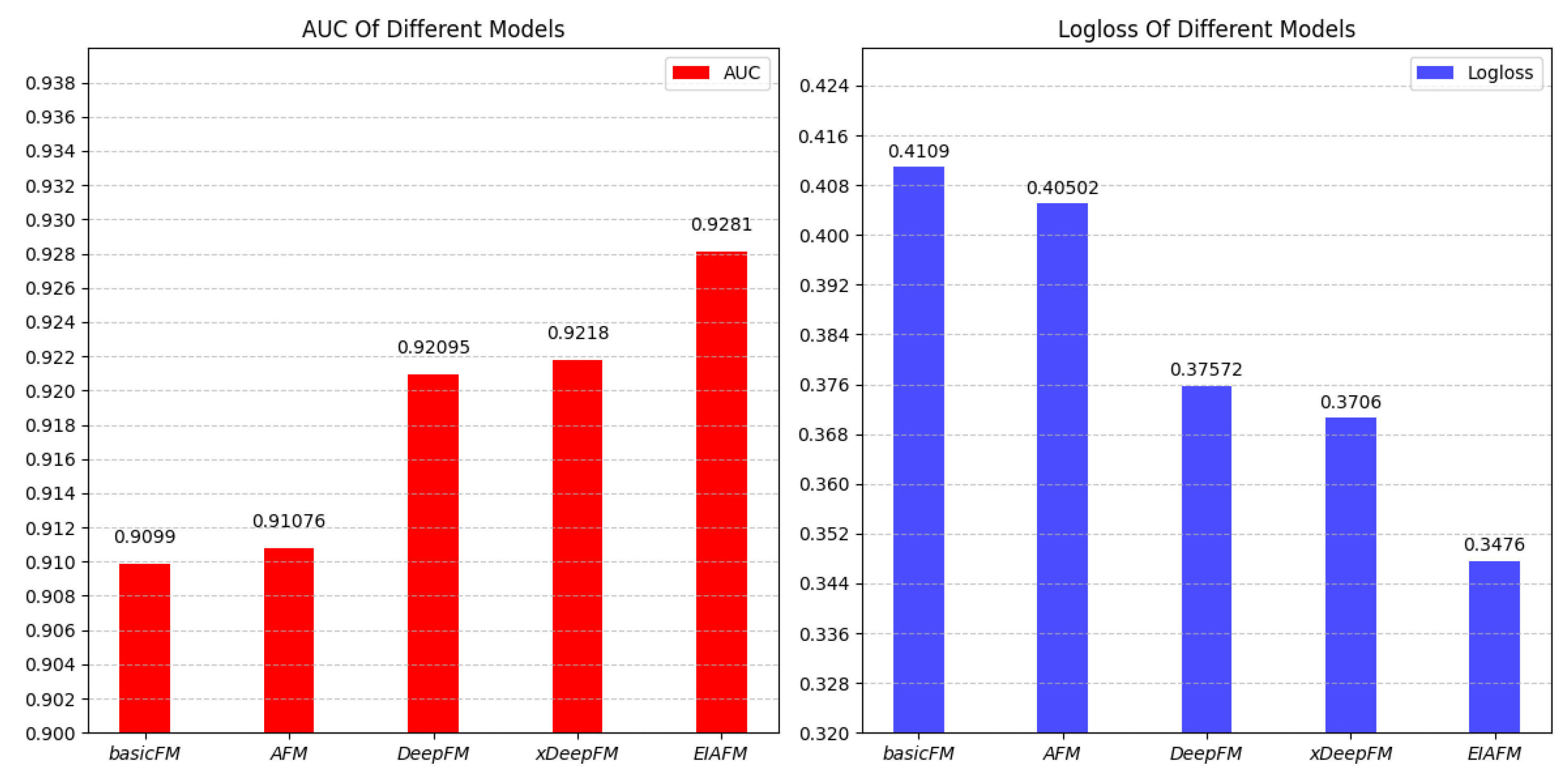
In theis experiment EIAFM was contrasted against other cutting-edge recommendation models, with the difference in their model performance represented in Figure 3:

Figure 3. Contrasting the EIAFM model with FM-based models in terms of service recommendation performance.

From Figure 3, it can be seen that EIAFM performs the best in terms of the log-loss and AUC metrics; xDeepFM performs the next best, followed by DeepFM, while basicFM performs the worst. AFM shows improved performance, indicating that measuring the varying importance of the second-order crossover is effective, and xDeepFM compares much better with the other models, which suggests that it is important to take into account both explicit and implicit higher-order feature interactions. The AUC values and log-loss of EIAFM show a significant improvement in model performance, and EIAFM is more effective than any other advanced FM-based recommendation model. Hence, mastering both explicit and implicit interactions of higher order features while quantifying the varying significance of second-order interactions can lead to a substantial enhancement of the model’s recommendation capabilities.

5.3.2. Analysis and Comparison of Model Complexity and Runtime

To further explore the efficiency of various recommendation models, our experiments were conducted on a dataset aligning with the industrial software component recommendation problem. This enabled comparison of the complexity and model parameter size of FM-based models currently utilized in the field of recommendation. The configuration parameters in the dataset used for comparison were as follows: the DNN had a depth of H = 2, with U = 32 hidden units, utilizing a = 32 attention factors and an embedding size of E = 32, while the CIN had a depth of T = 2 with F = 4 hidden units and the dataset contained N = 104 features. From Table 4, it can be observed that the model complexity of EIAFM is slightly higher than that of other models, while parameter size is the same as that of AFM. This is due to the inputs of the implicit and attention components designed in this paper utilizing feature interactions in common, which greatly reduces model complexity. Thus, EIAFM combines all the above-mentioned advantages without increasing model complexity. In terms of model complexity, EIAFM has lower complexity than AFM and xDeepFM combined. Furthermore, in terms of runtime, although EIAFM takes more time, it is faster than the combined runtimes of basicFM, xDeepFM, and AFM. In summary it can be inferred from the time complexity and runtimes that EIAFM can feasibly be used in industrial software service component recommendation scenarios.

Table 4. Complexity, parameter count, and runtime comparison of FM-based models.

Models	Complexity	Parameter Count	Runtime (Second)
basicFM	O(NE)	$3\times {10}^3$	1.0754
AFM	O(NE+N2E+EA)	$4\times {10}^6$	10.2260
DeepFM	O(NE+NEHU)	$1\times {10}^5$	2.5560
xDeepFM	O(NE+NEHU+NTF2)	$1\times {10}^5$	3.6041
EIAFM	O(NE+N2E+EHU+EA+NTF2)	$4\times {10}^6$	14.0392

5.3.3. Influence of Hyperparameters

EIAFM configures both the DNN and CIN with two hidden layers, and each hidden layer has an equal number of units. Only the number of units in each hidden layer needs to be investigated, as the dropout rates for the DNN, CIN, attention network output, and output of the pair-wise interaction layer are uniformly configured. All other hyperparameters were configured using their default values when exploring the effects of each parameter on the EIAFM model. Figure 4 shows the impact of the hyperparameters of EIAFM (number of DNN hidden units, attention factor, L2 regularization strength, dropout rate, and number of CIN hidden units).

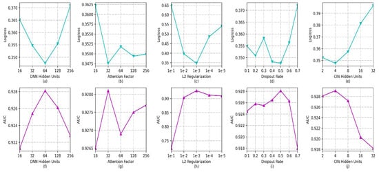
Figure 4. Effects of hyperparameters in EIAFM.

• The effect of the quantity of hidden units in the DNN: as observed in in Figure 4a,f, it can be seen that the log-loss value decreases sharply with the increase in the number of DNN hidden units; when the count of hidden units reaches 64, the log-loss value starts to rise sharply. The corresponding AUC value first rises sharply, then starts to fall when the count of hidden units reaches 64. More hidden units make the model more capable of nonlinear interactions. However, an excessive number of hidden units can lead to overfitting in the model. When the number of hidden units is in the range of [32,128], both the log-loss and AUC perform well.
• Effect of Attention Factor: from Figure 4b,g, it can be observed that the log-loss and AUC fluctuate slightly when the attention factor is greater than 32. This fluctuation is due to the fact that the role of the attention component is to use the attention weights to measure which feature interactions contribute more significantly to the prediction. For low attention factors, there exists only slight variability in the significance scores of various feature interactions. The log-loss and AUC fluctuate relatively little when the attention factor reaches 32, and overall the model works best at an attention factor of 32.
• Effect of L2 regularization and dropout rate: from Figure 4c,h, it can be observed that the log-loss decreases first and then increases, and the model achieves the best performance when the strength of L2 regularization is 1 × 10${}^{-3}$. The main purpose of L2 regularization is to avoid overfitting. The optimization of the loss function is affected when the L2 regularization reaches 1 × 10${}^{-1}$; the overall view is that the best results for both the log-loss and AUC are achieved when the strength of L2 regularization is 1 × 10${}^{-3}$. The effect of the dropout rate can be observed from Figure 4d,i; the effect of dropout rate is not very large for the model except for the setting of 0.7. The log-loss and AUC values perform poorly, as on average a larger dropout requires more iterations for the model training to converge for the experimental default number of iterations. The model exhibits peak performance when the dropout rate is configured as 0.5.
• The effect of the quantity of hidden layer units in CIN: as can be observed from Figure 4e,j, the log-loss first decreases and then grows drastically with the increase in the number of CIN hidden units. The reason for this is mainly that the increase in the quantity of neurons in each layer of the CIN results in an increase in the number of feature maps in the CIN. Though the model is better able to learn the information of feature interactions with different orders, too many of them increases the model’s complexity and produces overfitting. In addition, according to the experimental results, better results are obtained when the number of CIN hidden layers is 4. The main reason for this is that the CIN in the model design is a better complement to the DNN for high-order feature interactions, and does not need very many hidden layer units to achieve better training results. Another noteworthy observation is that the neural network-based model does not need a deeper network structure to obtain the best results; the best results can be obtained by setting the number of layers of both the CIN and DNN to 2 during the training process on this dataset.

5.3.4. Influence of Different Components in EIAFM

The model architecture of EIAFM covers different properties of feature learning. In order to investigate how EIAFM can increase model performance from the four components at the same time, the components of the model were changed from 1 to 4. The other hyperparameters were defaulted to match the values provided in Table 3, and the linear, attention, explicit, and implicit components are represent as LC, AC, EC, and IC, respectively. Fifteen different combinations of the components were obtained, and the experimental results are shown in Table 5. From the table, it can be seen that the model performance is optimal with four components, which captures the individual feature interaction components.

Table 5. Contrasting models with varied components in EIAFM.

Mode With Varied Components	Logloss	AUC
LC	0.413	0.9035
AC	0.4726	0.8933
EC	0.3897	0.918
LC + AC	0.4053	0.9106
LC + EC	0.3881	0.9104
LC + IC	0.3686	0.9187
AC + EC	0.3811	0.9138
AC + IC	0.3701	0.9165
EC + IC	0.3622	0.9211
IC + EC + AC	0.3501	0.9261
IC + AC + LC	0.3605	0.9239
IC + EC + LC	0.3595	0.9242
AC + EC + LC	0.3754	0.9155
LC + AC + EC + IC	0.3476	0.9281

It can be observed that EC performs best in the one-component model, which indicates that the explicit higher-order interactions between inputs and outputs are more important than the other relationships. EC + IC performs best in the two-component model, which indicates that the explicit and implicit higher-order interactions between the inputs and outputs are more effective than the other two-component combinations of the model; this conforms to the design idea behind the xDeepFM model. It is worth noting that the importance of the combination of EC and IC is used in the comparison of the three-component models; the key point is that IC + EC + AC is more effective compared to the IC + EC + LC model, as the former contains an attention component, indicating that the combination of explicit and implicit higher-order feature interactions and the attention component can improve the model performance. To summarize, it can be concluded that more components result in better model effectiveness and that each component contributes to the recommendation performance of the EIAFM model.

5.4. Discussion

First, our experimental results indicate that EIAFM significantly improves model performance in providing recommendations. During the model design process, as described in Section 5.3.4, we conducted relevant ablation experiments to explore the impact of the different aspects of feature interaction on model performance. Our experimental results suggest that simultaneously capturing explicit and implicit high-order interactions in recommendation models and introducing an attention mechanism to capture low-order interactions is effective. This approach aligns with the design principles of state-of-the-art related models; thus, we based our model architecture on this design.

Second, in exploring the model’s hyperparameters, as described in Section 5.3.3, we experimented with different numerical values to investigate their impact on model performance. This process helped us to select appropriate hyperparameter values. It is important to note that these experiments were conducted based on our training dataset; for future applications, parameter values may need to be adjusted according to the scale of the dataset.

Additionally, as observed in Section 5.3.2, while the EIAFM model shows improved recommendation performance, it increases model training time and the number of parameters. However, this increase is not significant compared to mainstream models. Therefore, EIAFM is applicable to the Service Recommendation of Industrial Software Components task.

Finally, the results of this experiment are of significant importance in the field of service recommendation. They offer a new approach that simultaneously captures explicit and implicit high-order interactions and introduces an attention mechanism to capture low-order interactions, providing valuable insights.

See Table 6 for a list of the abbreviations used in this article.

Table 6. Abbreviations.

SOA	Service-oriented architecture
DM	The descriptive information of the industrial task
SIM	The similarity between the service component and the industrial task
POC	The prevalence of the service component
CC	The class of the service component
CM	The class of the industrial task
S	The final prediction score
LC	Linear component
AC	Attention component
EC	Explicit component
IC	Implicit component

6. Conclusions

In this paper, a decomposer model based on explicit and implicit higher-order feature interactions and attention mechanisms is proposed. The proposed model uses a new architecture named EIAFM, with a DNN (the implicit component) used to capture higher-order implicit feature interactions and a CIN (the explicit component) used to capture higher-order explicit feature interactions. In addition, we introduce an attention module (the attention component) to capture the varying contributions of lower-order feature interactions to prediction results through attention weights, while the implicit and attention components both make use of identical input feature interaction data. The resulting recommendation architecture is designed for novel application scenarios targeting recommendation of industrial software service components, and the related problem is mathematically modeled. Extensive experiments were carried out on a problem-defined real dataset, with the results clearly indicating that EIAFM surpasses existing recommendation models. Based on our experiments, while the four components of EIAFM have different contributing effects, all improve the performance of the model and are helpful for improving the recommendation of industrial software service components.

In future work, combining the application of attention mechanisms in higher-order feature interactions will be investigated to improve the performance of the proposed model. In addition, in the definition of the recommendation problem for industrial software service components, the specific preferences of the user who publishes the industrial task are not taken into account, meaning that diverse personalized recommendation schemes can be considered. The recommendation architecture for industrial software service components proposed in this paper is flexible, and other relevant features included in the service recommendation can be selected to optimize the recommendation performance in the feature information network composed of industrial tasks and industrial software service components.

References

- Ding, D.; Han, Q.L.; Wang, Z.; Ge, X. A survey on model-based distributed control and filtering for industrial cyber-physical systems. IEEE Trans. Ind. Inform. 2019, 15, 2483–2499. [Google Scholar] [CrossRef]
- Shmeleva, A.G.; Ladynin, A.I. Industrial management decision support system: From design to software. In Proceedings of the 2019 IEEE Conference of Russian Young Researchers in Electrical and Electronic Engineering (EIConRus), Saint Petersburg and Moscow, Russia, 28–31 January 2019; pp. 1474–1477. [Google Scholar]
- Niknejad, N.; Ismail, W.; Ghani, I.; Nazari, B.; Bahari, M. Understanding Service-Oriented Architecture (SOA): A systematic literature review and directions for further investigation. Inf. Syst. 2020, 91, 101491. [Google Scholar] [CrossRef]
- Kutnjak, A.; Pihiri, I.; Furjan, M.T. Digital transformation case studies across industries–Literature review. In Proceedings of the 2019 42nd International Convention on Information and Communication Technology, Electronics and Microelectronics (MIPRO), Opatija, Croatia, 20–24 May 2019; pp. 1293–1298. [Google Scholar]
- Wu, L.; He, X.; Wang, X.; Zhang, K.; Wang, M. A survey on accuracy-oriented neural recommendation: From collaborative filtering to information-rich recommendation. IEEE Trans. Knowl. Data Eng. 2022, 35, 4425–4445. [Google Scholar] [CrossRef]
- Cui, Z.; Xu, X.; Fei, X.; Cai, X.; Cao, Y.; Zhang, W.; Chen, J. Personalized recommendation system based on collaborative filtering for IoT scenarios. IEEE Trans. Serv. Comput. 2020, 13, 685–695. [Google Scholar]
- Wang, W.; Chen, J.; Wang, J.; Chen, J.; Liu, J.; Gong, Z. Trust-enhanced collaborative filtering for personalized point of interests recommendation. IEEE Trans. Ind. Inform. 2019, 16, 6124–6132. [Google Scholar] [CrossRef]
- Rahman, M.M.; Liu, X.; Cao, B. Web API recommendation for mashup development using matrix factorization on integrated content and network-based service clustering. In Proceedings of the 2017 IEEE international conference on services computing (SCC), Honolulu, HI, USA, 25–30 June 2017; pp. 225–232. [Google Scholar]
- Xu, W.; Cao, J.; Hu, L.; Wang, J.; Li, M. A social-aware service recommendation approach for mashup creation. In Proceedings of the 2013 Ieee 20th International Conference on Web Services, Santa Clara, CA, USA, 28 June–3 July 2013; pp. 107–114. [Google Scholar]
- Yao, L.; Wang, X.; Sheng, Q.Z.; Benatallah, B.; Huang, C. Mashup recommendation by regularizing matrix factorization with API co-invocations. IEEE Trans. Serv. Comput. 2018, 14, 502–515. [Google Scholar] [CrossRef]
- Wang, Y.; Feng, D.; Li, D.; Chen, X.; Zhao, Y.; Niu, X. A mobile recommendation system based on logistic regression and gradient boosting decision trees. In Proceedings of the 2016 international joint conference on neural networks (IJCNN), Vancouver, BC, Canada, 24–29 July 2016; pp. 1896–1902. [Google Scholar]
- Cao, B.; Liu, J.; Wen, Y.; Li, H.; Xiao, Q.; Chen, J. QoS-aware service recommendation based on relational topic model and factorization machines for IoT Mashup applications. J. Parallel Distrib. Comput. 2019, 132, 177–189. [Google Scholar] [CrossRef]
- Zhang, X.; Liu, J.; Cao, B.; Xiao, Q.; Wen, Y. Web service recommendation via combining Doc2Vec-based functionality clustering and DeepFM-based score prediction. In Proceedings of the 2018 IEEE Intl Conf on Parallel & Distributed Processing with Applications, Ubiquitous Computing & Communications, Big Data & Cloud Computing, Social Computing & Networking, Sustainable Computing & Communications (ISPA/IUCC/BDCloud/SocialCom/SustainCom), Melbourne, VIC, Australia, 11–13 December 2018; pp. 509–516. [Google Scholar]
- Cao, B.; Li, B.; Liu, J.; Tang, M.; Liu, Y. Web apis recommendation for mashup development based on hierarchical dirichlet process and factorization machines. In Proceedings of the Collaborate Computing: Networking, Applications and Worksharing: 12th International Conference, CollaborateCom 2016, Beijing, China, 10–11 November 2016; Proceedings 12. Springer: Berlin/Heidelberg, Germany, 2017; pp. 3–15. [Google Scholar]
- Sedhain, S.; Menon, A.K.; Sanner, S.; Xie, L. Autorec: Autoencoders meet collaborative filtering. In Proceedings of the 24th international conference on World Wide Web, Florence, Italy, 18–22 May 2015; pp. 111–112. [Google Scholar]
- Cheng, H.T.; Koc, L.; Harmsen, J.; Shaked, T.; Chandra, T.; Aradhye, H.; Anderson, G.; Corrado, G.; Chai, W.; Ispir, M.; et al. Wide & deep learning for recommender systems. In Proceedings of the 1st Workshop on Deep Learning for Recommender Systems, Boston, MA, USA, 15 September 2016; pp. 7–10. [Google Scholar]
- Guo, H.; Tang, R.; Ye, Y.; Li, Z.; He, X. DeepFM: A factorization-machine based neural network for CTR prediction. arXiv 2017, arXiv:1703.04247. [Google Scholar]
- Vaswani, A.; Shazeer, N.; Parmar, N.; Uszkoreit, J.; Jones, L.; Gomez, A.N.; Kaiser, Ƚ; Polosukhin, I. Attention is all you need. Adv. Neural Inf. Process. Syst. 2017, 30. [Google Scholar]
- Barkan, O.; Koenigstein, N. Item2vec: Neural item embedding for collaborative filtering. In Proceedings of the 2016 IEEE 26th International Workshop on Machine Learning for Signal Processing (MLSP), Vietri sul Mare, Italy, 13–16 September 2016; pp. 1–6. [Google Scholar]
- Wang, F.; Zhu, H.; Srivastava, G.; Li, S.; Khosravi, M.R.; Qi, L. Robust collaborative filtering recommendation with user-item-trust records. IEEE Trans. Comput. Soc. Syst. 2021, 9, 986–996. [Google Scholar] [CrossRef]
- Sun, J.; Zhang, Y.; Ma, C.; Coates, M.; Guo, H.; Tang, R.; He, X. Multi-graph convolution collaborative filtering. In Proceedings of the 2019 IEEE International Conference on Data Mining (ICDM), Beijing, China, 8–11 November 2019; pp. 1306–1311. [Google Scholar]
- Shen, D.; Liu, J.; Wu, Z.; Yang, J.; Xiao, L. ADMM-HFNet: A matrix decomposition-based deep approach for hyperspectral image fusion. IEEE Trans. Geosci. Remote Sens. 2021, 60, 5513417. [Google Scholar] [CrossRef]
- Li, C.; Jiang, T.; Wu, S.; Xie, J. Single-channel speech enhancement based on adaptive low-rank matrix decomposition. IEEE Access 2020, 8, 37066–37076. [Google Scholar] [CrossRef]
- Yang, B. Application of Matrix Decomposition in Machine Learning. In Proceedings of the 2021 IEEE International Conference on Computer Science, Electronic Information Engineering and Intelligent Control Technology (CEI), Fuzhou, China, 24–26 September 2021; pp. 133–137. [Google Scholar]
- Richardson, M.; Dominowska, E.; Ragno, R. Predicting clicks: Estimating the click-through rate for new ads. In Proceedings of the 16th International Conference on World Wide Web, Banff, AB, Canada, 8–12 May 2007; pp. 521–530. [Google Scholar]
- Chang, Y.W.; Hsieh, C.J.; Chang, K.W.; Ringgaard, M.; Lin, C.J. Training and testing low-degree polynomial data mappings via linear SVM. J. Mach. Learn. Res. 2010, 11, 1471–1490. [Google Scholar]
- Juan, Y.; Zhuang, Y.; Chin, W.S.; Lin, C.J. Field-aware factorization machines for CTR prediction. In Proceedings of the 10th ACM Conference on Recommender Systems, Boston, MA, USA, 15–19 September 2016; pp. 43–50. [Google Scholar]
- Shan, Y.; Hoens, T.R.; Jiao, J.; Wang, H.; Yu, D.; Mao, J. Deep crossing: Web-scale modeling without manually crafted combinatorial features. In Proceedings of the 22nd ACM SIGKDD International Conference on Knowledge Discovery and Data Mining, San Francisco, CA, USA, 13–17 August 2016; pp. 255–262. [Google Scholar]
- Qu, Y.; Cai, H.; Ren, K.; Zhang, W.; Yu, Y.; Wen, Y.; Wang, J. Product-based neural networks for user response prediction. In Proceedings of the 2016 IEEE 16th International Conference on Data Mining (ICDM), Barcelona, Spain, 12–15 December 2016; pp. 1149–1154. [Google Scholar]
- Wang, R.; Fu, B.; Fu, G.; Wang, M. Deep & cross network for ad click predictions. In Proceedings of the ADKDD’17, Halifax, NS, Canada, 14 August 2017; pp. 1–7. [Google Scholar]
- Zhang, W.; Du, T.; Wang, J. Deep Learning over Multi-field Categorical Data: A Case Study on User Response Prediction. In Proceedings of the Advances in Information Retrieval: 38th European Conference on IR Research, ECIR 2016, Padua, Italy, 20–23 March 2016; Proceedings 38. Springer: Berlin/Heidelberg, Germany, 2016; pp. 45–57. [Google Scholar]
- Lian, J.; Zhou, X.; Zhang, F.; Chen, Z.; Xie, X.; Sun, G. xdeepfm: Combining explicit and implicit feature interactions for recommender systems. In Proceedings of the 24th ACM SIGKDD International Conference on Knowledge Discovery & Data Mining, London, UK, 19–23 August 2018; pp. 1754–1763. [Google Scholar]
- Xiao, J.; Ye, H.; He, X.; Zhang, H.; Wu, F.; Chua, T.S. Attentional factorization machines: Learning the weight of feature interactions via attention networks. arXiv 2017, arXiv:1708.04617. [Google Scholar]
- Kang, G.; Liu, J.; Cao, B.; Cao, M. Nafm: Neural and attentional factorization machine for web api recommendation. In Proceedings of the 2020 IEEE international conference on web services (ICWS), Beijing, China, 19–23 October 2020; pp. 330–337. [Google Scholar]
- Kang, G.; Liu, J.; Xiao, Y.; Cao, B.; Xu, Y.; Cao, M. Neural and attentional factorization machine-based Web API recommendation for mashup development. IEEE Trans. Netw. Serv. Manag. 2021, 18, 4183–4196. [Google Scholar] [CrossRef]
- Le, Q.; Mikolov, T. Distributed representations of sentences and documents. In Proceedings of the International Conference on Machine Learning, PMLR, Montreal, QC, Canada, 8–13 December 2014; pp. 1188–1196. [Google Scholar]
- Huang, K.; Fan, Y.; Tan, W. An empirical study of programmable web: A network analysis on a service-mashup system. In Proceedings of the 2012 IEEE 19th International Conference on Web Services, Honolulu, HI, USA, 24–29 June 2012; pp. 552–559. [Google Scholar]
Disclaimer/Publisher’s Note: The statements, opinions and data contained in all publications are solely those of the individual author(s) and contributor(s) and not of MDPI and/or the editor(s). MDPI and/or the editor(s) disclaim responsibility for any injury to people or property resulting from any ideas, methods, instructions or products referred to in the content. |
© 2023 by the authors. Licensee MDPI, Basel, Switzerland. This article is an open access article distributed under the terms and conditions of the Creative Commons Attribution (CC BY) license (https://creativecommons.org/licenses/by/4.0/).