Combined Optimization of Maintenance Works and Crews in Railway Networks

Abstract

This study develops optimal maintenance schedules for train lines, a critical endeavor ensuring the safety, efficiency, and reliability of railway networks. The study addresses the combined scheduling problem of maintenance works and crews on the railway networks. The baseline scheduling model is initially established with the primary objective of allocating maintenance tasks efficiently while adhering to pertinent constraints, encompassing task grouping and cost minimization. Subsequently, this baseline model is enhanced through the integration of crew scheduling, wherein work crews are strategically assigned to execute predefined tasks, thereby facilitating effective workload distribution. The combined maintenance work and crew scheduling problem is mathematically formulated as a binary linear programming model, enabling the attainment of globally optimal solutions. Comparing the outcomes of our enhanced model, which incorporates both maintenance works and crew schedules, with the baseline model that solely addresses maintenance works, we reveal that task grouping in accordance with predefined conditions leads to reduced overall costs by minimizing maintenance duration during various periods. Additionally, the judicious distribution of workload among the crews ensures comprehensive coverage of all essential tasks. These findings underscore the significance of our proposed approach in enhancing the operational efficacy and economic viability of railway maintenance scheduling, thereby offering valuable insights for practical implementation and future research endeavors.

1. Introduction

Transportation is a vital sector for society, as it profoundly influences daily citizen services and the economy. Notably, the railway sector has evolved into one of the safest and most environmentally friendly modes of transportation, encompassing primarily freight and passenger transport. The global railway network spans over an extensive 1.3 million kilometers worldwide, with the United States boasting the longest railway network, while Japan earned recognition for having the highest quality of railway infrastructure in 2019 [1]. Analyzing statistics from 2015 to 2021, it is evident that the demand for railway passenger transport experienced significant growth in the European Union until 2019. From 2019 to 2021 the statistics show a remarkable drop due to the pandemic of COVID-19 [2]. For instance, in 2016, Germany recorded the highest number of railway passenger trips, estimated at around 2.8 billion passengers [3]. Furthermore, Rail Freight Forward, representing a substantial 90% of Europe’s rail freight transport, aims to elevate the share of railway freight transport from 18% to 30% by the year 2030. This ambitious goal has the potential to reduce approximately 25 million tons of CO₂ emissions [4]. Nonetheless, the prevailing requirements necessitate the railway industry to augment its capacity by introducing more trains with higher speeds and greater carrying capabilities. However, this progression comes with a drawback, as it leads to the deterioration of railway infrastructure and escalates maintenance costs. European countries allocate a significant sum, approximately EUR 15 to 25 billion annually, towards the maintenance and renovations of their railway systems [5]. These financial commitments underscore the importance of sustaining and enhancing the railway network to meet evolving demands while ensuring its long-term efficiency and environmental sustainability.

The railway infrastructure should provide dependable conditions, thereby circumventing substantial disruptions in both passenger and freight transport operations. As such, the primary objective of railway line maintenance is to attain consistently high standards of safety and functionality while optimizing both time and cost factors. The economic significance of maintenance also becomes evident, as evidenced by the European railway network’s expenditure, which surpassed EUR 25 billion in 2016, compared to EUR 20 billion in 2011. Notwithstanding this noteworthy cost escalation, budgets allocated for railway maintenance remain constrained, compelling infrastructure operators throughout the continent to explore strategies for accomplishing more with limited resources and achieving improved control over maintenance expenses [6].

Maintenance activities within the railway infrastructure can be broadly categorized into two main groups: inspection, which involves identifying and evaluating the current condition of the infrastructure, and restoration, focusing on rectifying already identified defects. Regular inspections are conducted at predetermined intervals, while emergency inspections occur to prevent potential incidents or address observed abnormalities during train operations. Special inspections are carried out at specific points with known risks, such as areas prone to landslides. The frequency of consecutive regular inspections adheres to predetermined time intervals. Restoration works can be further divided into three categories: material maintenance, which entails the replacement of sleepers, rails, and fastening elements; geometry maintenance works, involving track lifting and realignment; and ongoing maintenance tasks, such as leveling and aligning the track and lubricating switch points. Vale et al. [7] focused on the preventive maintenance of railway tracks with ballast for compression works, and their model allows the analysis of maintenance actions over time, with longer analysis periods leading to better maintenance planning. Lidén [8] categorized maintenance activities based on the required time of possession per work shift, emphasizing the significance of time frames in maintenance scheduling to ensure the timely restoration of infrastructure. However, Lidén [9] pointed out a conflict in railway infrastructure management concerning the coordination of train traffic with maintenance activities, particularly in networks with a high traffic density. Balancing both becomes crucial, and often maintenance is scheduled during periods of minimal or no train schedule, including nighttime hours with fewer passenger movements. Dao et al. [10] dealt with major and significant maintenance planning, as well as renewal processes, highlighting their complexity and involving multiple stakeholders, such as the railway infrastructure manager, train operating company, traffic control, and maintenance contractors. Conversely, Vansteenwegen et al. [11] proposed an algorithm that could adjust the train’s route and timetable to accommodate scheduled maintenance tasks while maintaining passenger service levels to as high a degree as possible. The algorithm aimed to minimize the number of cancelled train schedules, and the results indicated that minor adjustments could significantly reduce the need for cancellations.

It should be noted that the frequency of actions required in maintenance, inspection, and restoration, whether predetermined or not, depends on a range of factors, with the most critical ones being the train’s traffic volume, speed, and weight. Therefore, when exceeding a critical degradation value of the railway track, corrective measures should be taken immediately. In this study, we propose a model for the combined scheduling of maintenance works and crew schedules. The remainder of this study is structured as follows. Section 2 presents the relevant literature. Section 3 introduces the problem description and the mathematical formulation of our model. The implementation, the results, and the conclusions are presented in Section 4, Section 5 and Section 6, respectively.

2. Related Studies

In recent years, significant research studies have been undertaken to investigate the optimal railway maintenance scheduling. The approach by S. M. Pour et al. [12] focused on allocating the maintenance tasks in the Jutland peninsula, the largest region in Denmark, to a set of maintenance crew members, where each crew undertakes a sub-region. The goal was to minimize the distance between two different tasks in the same sub-region by proposing a perturbative hyper-heuristic framework.

Dotoli et al. [13] presented a Decision Support System (DSS) applied in a real dataset in Southern Italy. The problem aimed to reschedule the timetable in real time and solve conflicts in the network for unexpected disturbances. The objective was to minimize the cost of delays.

A different study was conducted by Sedghi et al. [14] which intended to discuss current literature approaches for optimization in maintenance planning and scheduling, including possible gaps related to decision-making models. One of the observations was about the decision support models that are cost-based which often combine various costs to minimize the overall cost. Regarding the cost, they expect a stronger emphasis on environmental and other sustainability-related costs.

In their study, Cavone et al. [15] proposed an automatic rescheduling algorithm for the real-time control of railway traffic and tested it in simulation on the Dutch railway network. The scope of this was to minimize the delays caused by disruptions. They used a Model Predictive Control (MPC) algorithm, while the rescheduling problem was solved by mixed integer linear programming using macroscopic and mesoscopic models.

Cavone et al. [16] developed a model that focuses on disruptions tested in the Dutch railway traffic system, proposing an innovative bi-level rescheduling algorithm based on a mesoscopic mixed integer linear programming. The technique manages to obtain a feasible rescheduled timetable in a short computation time including safety constraints and capacity.

An approach for the preventive signal maintenance crew scheduling problem in the Danish railway system was conducted by S. M. Pour et al. [17], which was formulated as a mixed integer optimization model. The objective was to minimize the number of working days, to ensure that as many tasks as possible are completed inside the planning horizon and to minimize the penalty for assigning crew members. Another study by S. M. Pour et al. [18] developed a model for planning preventive maintenance in the railway signaling system in Denmark. The problem was formulated as a multi-depot vehicle routing and scheduling problem with time windows and synchronisation constraints. Some tasks require the simultaneous presence of more than one engineer, which requires the consideration of task synchronization. Furthermore, a constraint programming (CP) approach was used to create viable monthly schedules for substantial, practically relevant scenarios, while the experimental results indicated that the proposed framework can generate feasible solutions and can schedule up to 1000 tasks for a monthly plan of eight crew members.

Apart from the conventional optimization approaches for railway operations and maintenance, there exist solutions using Artificial Neural Networks (ANN). First, in the study of Martinelli and Teng [19], the Train Formation Problem (TFP) was formulated as a Back-Propagation Neural Network (BPNN) model consisting of three layers: the input layer representing O-D demands, a hidden layer, and the output layer representing the trains with the assigned demand. Their main objective was to utilize neural networks for obtaining near-optimal solutions in short periods of time, due to the high computational time of conventional solution algorithms producing train formation plans. Furthermore, Gençer et al. [20] were the first to implement maintenance planning for metro trains with an ANN model incorporating all train equipment and factors affecting the failure. Within the artificial neural network model, five variables (equipment type, preventive maintenance frequency, material quality, life cycle, line status) were included as input factors which influence equipment faults, while the outputs were represented by the number of failures. Lastly, Popov et al. [21] used an Artificial Intelligence (AI) technique to analyze the track quality big data of a high-speed line in the UK, using a dataset with more than 15 years of track geometry. More specifically, an ANN model was developed to identify segments of the railway track where the condition was either improved or deteriorated during the time elapsed between two inspection runs.

2.1. Optimization of Railway Line Maintenance Scheduling

One area of research is concerned with the scheduling of maintenance operations to prevent disruptions to and from scheduled train routes, while also devising strategies to minimize infrastructure downtime and reduce maintenance costs. The study by Higgins [22] addressed the conflict between maintenance task scheduling and assigning them to crews within a given timetable. The goal was to achieve the optimal distribution of maintenance and crew activities to minimize disruptions to scheduled routes and reduce their duration. Higgins’s [22] approach was a heuristic tabu search for the order of tasks and maintenance crews. The model had specific constraints concerning the available budget, priority of maintenance activities, line availability, and minimum travel time between connecting lines.

Cheung et al. [23] dealt with the optimization of resource allocation for task execution. They used the constraint language CHIP to solve real-world resource allocation problems. The problem aimed to map railroad lines to a given set of scheduled maintenance tasks, subject to certain constraints. As an example of the model’s constraints, one involved the requirement to ensure that resources remained within the available limit. Another objective was to create a framework that maximizes task assignments based on their pre-defined priority.

The approach by Budai and Dekker [24] focused on preventive maintenance by exploring optimal track possession intervals for task execution. They mainly utilized train-free periods, resulting in a 33% reduction in track possession and associated costs, by combining works. Additionally, Budai et al. [25] emphasized grouping small routine works and larger projects, scheduling them within specific periods to minimize maintenance costs without burdening train traffic. They employed mathematical programming formulations and heuristic solutions due to the complexity of the problem. In contrast to the previously mentioned studies, Peng and Ouyang [26] investigated the scheduling of a maintenance crew where various maintenance tasks were to be scheduled for a set of maintenance groups. One of the constraints was related to the direction a maintenance group followed during the execution of a task, i.e., from one task to the next. Furthermore, a constraint was defined that each task can be executed exactly once by a maintenance crew.

Heinicke et al. [27] adopted a completely different approach, where maintenance tasks incur penalties in the form of costs until the specific task is completed. The longer the task execution time, the higher the penalty cost was. The problem was formulated as a Vehicle Routing Problem (VRP), developing, and comparing it with different Mixed-Integer Linear Programming (MILP) models and customer costs concerning the time of execution. It should be noted that the vehicle routing problem of this study, unlike the common VRPs, minimized the sum of travel expenses and customer costs that depend on time.

On the other hand, Van Zante-De Fokkert et al. [28] created a model in which each segment of the infrastructure was made available for maintenance at least once every four weeks. The main objective was to minimize maintenance costs. They defined a Single-Track Grid (STG), which is a traffic management system for railroad lines consisting of a single track. In this system, they divided the railroad line into work zones between stations, where each work zone defined a segment of the line for maintenance tasks which could be taken out of service for train traffic. They then utilized a Mixed-Integer Programming (MIP) model to define the single-track grids in shifts to create the maintenance schedule.

Another study focusing on minimizing maintenance costs was conducted by Lake et al. [29], who modelled short-term track maintenance scheduling within an existing timetable and maintenance program. The model included not only the tasks but also the assignment of tasks to maintenance crews. Different crews had the option to handle the same maintenance activity at different time periods. The model was solved with the introduction of a two-stage heuristic solution. The first stage generated a feasible solution, while the second stage used simulated annealing. Regarding the crews and worker safety, it is important to mention the research by Den Hertog et al. [30], where the division of the railway infrastructure into work zones was studied. The specific maintenance zone should be taken out of service, to satisfy all other factors involved. In this research, division rules were utilized that were developed for the Dutch network.

In their study, Andrade and Teixeira [31] set two objectives: maintenance cost and train delays. They focused on the track degradation model and decided whether maintenance should be performed or not. They utilized an optimization and simulation-based technique with two objectives for solving the problem. In more recent research, Su et al. [32] developed a Model Predictive Control (MPC) algorithm. At a higher level, their study determines the long-term maintenance plan per segment and minimizes maintenance costs and infrastructure degradation over a finite planning horizon. It ensured that the level of degradation of each segment remained above the maintenance threshold. At a lower level, the short-term maintenance tasks proposed by the high-level controller and the optimal routing of the corresponding maintenance crew were configured as a capacitated arc routing problem.

Nijland et al. [33] developed an optimization model for the maintenance scheduling for railway operators and maintenance crews. They also categorized the maintenance engineering sectors as they pose obstacles to train circulation and maintenance management. The method used was a novel mixed-integer linear programming model. Additionally, they evaluated the computational cost using exact (branch-and-bound) or heuristic solutions for solving networks with up to 25 work zones. Furthermore, Oudshoorn et al. [34] investigated a real railway maintenance scheduling problem for a one-year preventive maintenance period. They developed and compared three heuristic/metaheuristic approaches: evolutionary strategy, greedy heuristic, and a combination of both. The results showed that the best solution, providing a high-quality schedule, was achieved through the combination of strategic and greedy heuristic approaches.

Buurman et al. [35] focused on optimizing the maintenance schedule for railway operators and maintenance contractors with flexibility for both. The main factors to overcome obstacles were bypassing, rescheduling trains, and repositioning parked rolling stock. Their study explored the creation of a weekly recurring preventive maintenance program during the night to minimize train circulation delays as much as possible. They used a heuristic approach to find feasible solutions for large networks and an ε-constraint method for smaller networks.

2.2. Optimization of Maintenance Scheduling to Minimize the Impact on Circulation

Equally important are optimization techniques that incorporate time windows for railway maintenance, since many models do not consider train circulation. For this reason, Bueno et al. [36] used a simulated annealing solution as a basis for their algorithm, which produced results when using random block placements. The constraints were related to the initial time of a track block and the most recent finishing time of a track block, considering crew working hours. Moreover, Lidén and Joborn [37] emphasized the significance of railway services and the maintenance of the railway network, as they needed to be considered together in their planning. They presented a mixed-integer programming model for solving railway circulation and network maintenance. Their objective was to find a long-term plan that optimally schedules train-free windows for a specific volume of spatial and temporal aggregation for network capacity.

D’Ariano et al. [38] addressed the problem of regular scheduling to optimize train routing decisions, temporally correlated with short-term maintenance tasks in railway networks. They used a MILP model, incorporating stochastic variables, constraints, and objectives related to the flow of train circulation and track maintenance. Two objectives were set: one focused on minimizing deviations from a scheduled timetable, and the other on maximizing the consolidation of maintenance tasks.

In long-distance railway networks, maintenance and train routing scheduling are highly complex, especially in single-track networks. Building upon this issue, Albrecht et al. [39] investigated the Problem Space Search (PSS) through metaheuristic approaches, rapidly creating many alternative train routes and a timetable incorporating track maintenance. The approach of Forsgren et al. [40] was very close to this, using a MIP model to optimize train schedules and preventive maintenance. The model allowed train rerouting or cancellation to achieve the best possible traffic flow, considering a fixed set of scheduled maintenance activities. An overview of the most relevant reviewed studies is provided in Table 1.

Table 1. Relevant Studies.

Authors (Year)	Objective	Mathematical Formulation	Solution Method	Application
Higgins (1998) [22]	Minimize a weighted combination of expected interference delays with the train schedule and prioritized finishing time	Integer programming	Tabu search, Metaheuristics approaches	Artificial network
Cheung et al. (1999) [23]	Maximize the assignment of job requests based on priorities (as many higher-priority job requests as possible)	Chip constraint programming language	Heuristics approaches	Case study (Hong Kong, China)
Budai et al. (2006) [25]	Minimize the track possession time or cost for routine maintenance works and projects	Mixed-integer programming	(Greedy) Heuristics approaches (max to min, min to max, combined all in the first period)	Artificial network
Budai and Dekker (2004) [24]	Minimize the time periods for maintenance work, possession cost and cost for scheduled projects	Integer-linear programming	Exact solution (GAMS)	Artificial network
Peng and Ouyang (2012) [26]	Minimize the summation of all costs	Mixed-integer programming and customized search algorithms	Heuristics approaches	Case study (Class I railroad)
Heinicke et al. (2015) [27]	Minimize the sum of travel costs and customer costs	Mixed-integer-linear programming	Exact Solution (CPLEX)	Artificial network
Van Zante-De Fokkert et al. (2007) [28]	Minimize the number of nights with planned maintenance in the schedule, and the sum of the maximum scheduled workload of the contractors	Mixed-integer programming	Exact solution (AIMMS, CPLEX)	Artificial network
Lake et al. (2000) [29]	Minimize the cost of conducting the track maintenance	Mixed-integer nonlinear programming	Heurist approaches: (1) Feasible solution, (2) Simulated annealing	Case study (Queensland, Australia)
Andrade and Teixeira (2011) [31]	Minimize the total costs of planned maintenance and renewal actions and the total number of train delays caused by speed restrictions	Bi-objective integer nonlinear programming	Metaheuristics (Simulated annealing technique)	Artificial network
Su et al. (2019) [32]	Minimize the trade-off between condition deterioration and maintenance costs	Mixed-integer-linear programming	Scenario-based approach, Robust scenario-based approach	Case study (Randstad south and middle-south region, The Netherlands)
Nijland et al. (2021) [33]	Minimize the workload for work crews and the hindrance of train operators by minimizing the maximum workload of all crews combined	Mixed-integer-linear programming	Exact solution (branch-and-bond) Metaheuristics (Simulated annealing)	Case study (The Netherlands)
Oudshoorn et al. (2022) [34]	Representing total costs and exploring the trade-off between this cost and the number of hard constraint violations	Constraint programming model	Evolution strategy, greedy metaheuristic, a hybrid of the two	Case study (The Netherlands)
Lidén and Joborn (2017) [37]	A cost sum to be minimized for 5 cost components	Mixed-integer-linear programming	Exact solution (GUROBI)	Artificial network
D’Ariano et al. (2019) [38]	Minimize the total deviation from the nominal timetable. Maximize the number of paired works	Mixed-integer-linear programming Bi-objective model	Exact solution (IBM-ILOG-CPLEX)	Artificial network
Albrecht et al. (2013) [39]	Minimize the sum of train and maintenance delays	Problem Space Search (PSS)	Metaheuristics	Case study (Queensland, Australia)
Forsgren et al. (2013) [40]	Minimize the number of resource conflicts and cancelled trains	Mixed-integer-programming	Exact solution (CPLEX)	Case study (Sweden)
Buurman et al. (2023) [35]	Minimize the cost caused by hindrance over train operators. Maximize the number of scheduled slots in the maintenance schedule.	Multi-objective model, Integer-linear programming	Metaheuristic and e-constraint method	Case study (The Netherlands)
Bueno et al. (2019) [36]	Allocate time windows for railroad track maintenance to minimize the impact on train circulation	No formulation	Metaheuristic—Simulated Annealing for Track-block Optimization (SATO), Train Scheduling Planner (TSP)	Artificial network
Den Hertog et al. (2005) [30]	Divide the Dutch railway infrastructure into working zones	No formulation	Optimal rules for the working zone division	Artificial network
Dao et al. (2018) [10]	Minimize total cost in the whole planning horizon	Integer-linear programming	Exact solution (CPLEX)	Artificial Network
Vansteenwegen et al. (2016) [11]	Minimize the number of cancelled trains and minimize the decrease in service level to the passenger	Linear programming	Robust approach	Case study (Brussels, Belgium)

This study focuses on examining the problem of scheduling a one-year preventive maintenance work plan. The goal is to identify the specific tasks and their corresponding time periods required to complete them, all aimed at minimizing the overall downtime of the infrastructure due to maintenance activities. In addition, we aim to provide a higher efficiency of operations, grouping them in the best possible way in terms of economic benefit and efficiency and balancing the workload for the maintenance crews. The maintenance works included in this study refer to two types, short-term/routine works (e.g., track and switching inspection, railway inspection, signaling systems, switch lubrication) and long-term/project works (e.g., ballast cleaning, rail grinding, compaction). Long-term works require more time to complete than routine works and are usually carried out once/twice in a few years. From the reviewed studies, the closest prior comparator to our work is the study of Budai and Dekker [24] which we use as a baseline model. Budai and Dekker [24] scheduled only the maintenance works, whereas our approach schedules the maintenance works and the crew schedules in combination. This results in an enhanced model, revealing that task grouping and a judicious distribution of maintenance crews can lead to reduced overall costs by minimizing maintenance duration during various periods.

3. Methodological Framework and Problem Formulation

In countries with a high frequency of train services, such as the Netherlands, maintenance activities are usually scheduled during the night to avoid major disruptions. Furthermore, certain long-duration works require the closure of the railway line and are scheduled during the night or at the weekends, or during low traffic volumes. In railway lines with a lower frequency, certain maintenance activities can be carried out during the day in free time gaps between two consecutive train passages. During a link closure for maintenance works, a rerouting must be planned, a detour from the main track route must be made, or the route must be cancelled. This depends primarily on the railway network topology of the location where the maintenance work is being conducted, and it constitutes one of the main reasons for timetable delays.

Starting from the baseline model of Budai and Dekker [24] which schedules the maintenance works, we focused on the integration and assignment of work crews to perform the scheduled tasks. This means that for every planned task at every time and each link, there must be a work crew available. In this configuration framework, a reference point was created for the start and end of the work crews, namely the depot. In this way, depending on the movement of the crews, their costs and their exact location can be calculated. Each crew must perform one of the three options that have been set. The three options refer to a crew staying at the same link, moving to a different link, or returning to the depot. The incorporation of the work crews into the baseline model holds significant importance, as it facilitates enhanced management of the annual preventive maintenance program. This is achieved by ensuring the availability of the necessary work crews and their associated costs from the outset. Additionally, it enables a comprehensive overview of planned maintenance works and provides time for implementing the necessary actions towards its execution. To develop the enhanced model, it was necessary to add to the base model new sets, parameters, decision variables, and constraints to meet our requirements. A configuration of the objective function was also carried out by including a new term.

The base model of Budai and Dekker [24] defined some tasks and links of the railway line. The tasks were divided into two categories, projects, and routine works. The projects involved maintenance works that took a long time to complete, and the link had to be taken out of service or carried out at the maximum train-free period length. On the other hand, routine works involved maintenance works with a shorter completion time and could be carried out in time gaps between the passage of two consecutive trains. The planning period was one year, i.e., T = 52 weeks. Moreover, a set of combined tasks for both projects and routine works was created, which could be performed simultaneously on the same link. In addition, it should be mentioned that there is a set of three options indicating the execution time of the projects.

Before proceeding to the formulation of the objective function and the constraints, the following definitions of sets are required.

3.1. Sets

• PA—set of projects;
• RA—set of routine works;
• L—set of network links;
• $A=PA\cup RA$—set of all maintenance works;
• T—planning horizon (time);
• $K=\left\{\mathrm{1,2},3\right\}$—set of options for execution times;
• $Comb \left\{(m, n, l)\right\}$—set of combinable works $m$ and $n$ at link $l$, $\forall m,n\in A and l\in L$;
• ${max}_l$—maximum length of the train-free period on link $l\in L$.

It must be noted here that projects and routine works have different frequencies and therefore different scheduling. First, the link on which the selected project will be executed must be defined and then its earliest and latest start determined. Further, the duration needed to complete the project is defined for three options of $k ϵ K$, and each option corresponds to a different duration. The k = 1 option allows the works to run at the maximum length of the free train period (once a day) on several consecutive days, the k = 2 option allows the project works to run on weekends by closing the link for 48 h, and the k = 3 option closes the link for several days or weeks. In addition, based on these three options, three different costs are generated: one fixed cost for each time the link is used for maintenance and two additional costs, which refer to the penalties for the cancelled routes with option k = 2 or k = 3. The advantage of this option is the efficient use of resources by the crews. The third cost refers to the inefficient use of resources with option k = 1 or k = 2, since activities in these two scenarios may be interrupted and equipment must be moved by the crews. Routine works are executed with a higher frequency and their frequency should be determined upfront. Based on the frequency and the scheduling period of a year, tasks can be allocated within the planning time horizon.

In addition, our enhanced model includes different links L corresponding to a crew E each time a task is scheduled. To include the set of crews E, we introduce their available number in our model and a set of links for the crews, in which we have added the depot as their reference point. In this way, when a crew is not performing a task, it returns to the depot, and thus the exact locations of the crews are known. The added sets are presented below:

• E—set of crews;
• LL—set of links for crews.

3.2. Parameters

• $G_{al}—$frequencies per T scheduling period of activities $a\in RA$ on link $l\in L$, where $G_{al}=0$ if the activity $a\in RA$ is not relevant to the link $l\in L$;
• $T{W}_{pl}—$total workload (in hours) for a long-term work/project $p\in PA$ on link $l\in L$;
• $I_{pl}—$0–1 values depending on whether a project $p\in PA$ will be performed on the link $l\in L$ during the scheduling period t $\in T$;
• $D_{kpl}—$the duration of a project $p\in PA$ on link $l\in L$ using option $k\in K$, with

$$D_{kpl}=ceil\left(\frac{TWpl}{7\cdot maxl}\right) \mathrm{if} k = 1,$$

(1)

$$D_{kpl}=ceil\left(\frac{TWpl}{48}\right) \mathrm{if} k = 2, \mathrm{and}$$

(2)

$$D_{kpl}=ceil\left(\frac{TWpl}{7\cdot 24}\right) \mathrm{if} k = 3$$

(3)

• $LSTpl—$the earliest possible starting time of project $p\in PA$ on link $l\in L$;
• $USTpl—$the latest possible starting time of project $p\in PA$ on link $l\in L$;
• $F_{al}—F_{al}=ceil(T/Gal)$is the planning cycle for each routine work $a\in RA$ at each different link $l\in L$;
• $C_{lt}—$cost for possession of link $l\in L$at time t$\in T$;
• ${CCost}_{kl}—$cancellation cost on link $l\in L$ using option $k\in K$;
• ${MCost}_{kpl}—$penalty cost for resource utilization if option $k\in K$ is chosen for performing project $p\in PA$ on link $l\in L$.

Contrary to the base model, our enhanced model searches and makes decisions for the work crews. For the execution of the maintenance tasks $a\in A$by the work crew $e\in E$, their availability for link $l\in L$ at every time $t\in T$ is predefined by the parameter ${{\rm Z}}_{ealt}$. Moreover, for moving from one link to another, a distance $W_{lq}$ is defined between the two links $l\in L$ and the work crew links $q\in LL$. In the case of two identical links, $W_{lq}$ will take a value of 0 since no movement distance is measured. Otherwise, it will take the value of 1, which corresponds to the kilometric distance defined and is added to the objective function. The added parameters to our enhanced model are described below:

• ${{\rm Z}}_{ealt}—$binary, indicates whether a work crew $e\in E$ can serve a link $l\in L$ at time $t\in T$, or not;
• $W_{lq}—$distance between two links.

To be able to distinguish which tasks will be executed, at which time, on which link, and whether the link is used for a task, we define the following binary decision variables that will be used in the problem formulation.

3.3. Decision Variables

• $X_{alt}—$indicates whether activity $a\in A$ on link $l\in L$ is assigned to time $t\in T$, or not;
• $M_{lt}—$denotes whether period $t\in T$ is used for preventive maintenance work, or not;
• $Y_{kplt}—$indicates whether the execution of project $p\in PA$ starts at time $t\in T$ on link $l\in L$ if option $k\in K$ is chosen, or not;
• $B_{kpl}—$indicates whether the execution of project $p\in PA$ on link $l\in L$ is conducted according to option $k\in K$, or not.

A decision variable $h_{ealt}$ was added to our enhanced model for a scheduled task to be performed by a crew. The decision variable is binary and is a prerequisite for the improvement of decisions in the implementation of a task by a particular work crew. If a decision is made not to carry out a task on a particular link by a crew at a given time, the decision variable will be denoted as 0. Conversely, if the value is set to 1, it signifies that the crew is required to execute the task on that link. The decision variable added to the enhanced formulation problem is given below:

• $h_{ealt}$—binary, indicating whether work crew $e\in E$ serves link $l\in LL$ at time $t\in T$ for task $a\in A$, or not.

3.4. Formulation of the Objective Function and Constraints

The track possession problem, considering the scheduling of maintenance works in railway networks is formulated as a mathematical optimization problem. The mathematical program can be written as follows.

$$Min{\sum }_{lϵL}{\sum }_{t\in T}{C}_{lt }\cdot M_{lt}+{\sum }_{kϵK}{\sum }_{pϵP}{\sum }_{lϵL}{B}_{kpl}\cdot D_{kpl}\cdot \left({CCost}_{kl}+{MCost}_{kpl}\right) s.t.$$

(4)

$${\sum }_{tϵT}^{}Xalt=Gal \forall a ϵ RA, lϵL$$

(5)

$${\sum }_{t\in T}^{}{X}_{plt}={\sum }_{k\in K}^{}{I}_{pl}\cdot D_{kpl}\cdot B_{kpl} \forall p\in PA, lϵL$$

(6)

$${{\rm X}}_{mlt}+X_{nlt}\le 1 \forall \in T,\left(m,n,l\right)\notin Comb$$

(7)

$${\sum }_{t=s}^{s+F_{al}}{X}_{alt}+{\sum }_{t=1}^{s+F_{al}-1}{X}_{alt} \le 1 \forall a \in RA, l\in L, s\in T$$

(8)

$${\sum }_{t=1}^{\left|T\right|-D_{kpl}+1}{Y}_{kplt}=B_{kpl } \forall p \in PA, l \in L, t \in \left({LST}_{pl, }{UST}_{pl}\right) k \in K$$

(9)

$${\sum }_{s=t}^{t+D_{kpl}-1}{X}_{pls} \ge D_{kpl} Y_{kplt } \forall p\in PA, l\in L, t\in T, t\le T-D_{kpl}+1, I_{pl}=1, k\in K$$

(10)

$${\sum }_{k\in K}^{}{B}_{kpl}=1 \forall p\in PA, l\in L$$

(11)

$$M_{lt} \ge X_{alt} \forall a\in A, l\in L, t\in T$$

(12)

$$X_{alt}\in \left\{\mathrm{0,1}\right\}, M_{lt}\in \left\{\mathrm{0,1}\right\}, Y_{kplt} \in \left\{\mathrm{0,1}\right\}, B_{kpl}\in \left\{\mathrm{0,1}\right\} \forall a\in A, t\in T, l\in L, k\in K$$

(13)

The objective function, Equation (4), minimizes the number of time periods for which major maintenance work is planned per planning horizon T and thus the possession cost and the cost of carrying out the scheduled projects. The constraints of Equations (5) and (6) ensure that all routine works and projects are respectively assigned to the correct number of time periods for each link. The constraint of Equation (7) ensures that the combinable tasks (either routine works or projects) can only be performed at the same time and on the same link. Moreover, the constraint of Equation (8) prohibits routine maintenance works from being executed in close time intervals to each other and between two consecutive occurrences of the same task there must be $F_{al}$ time periods. The constraint of Equation (9) guarantees that the starting time for performing a project is in the interval between the earliest and the latest possible starting time. The constraint of Equation (10) ensures that if the execution starting time for each project is selected, then the projects are assigned to subsequent intervals. One of the three execution options must be chosen to perform the specified projects. This is ensured by the constraint of Equation (11). The constraint of Equation (12) ensures that time $t\in T$ will be used for preventive maintenance work if and only if there is at least one activity planned for that time in one of the segments. Finally, the constraint of Equation (13) ensures that the decision variables in the model are binary.

The above-formulated problem was extended to incorporate crews and optimize the scheduling assignment of work crews to maintenance tasks. The objective function of our enhanced model aims to minimize and allocate the workload for the crews through the decision variable $H_{ealt}$ and the cost required for their movements between two consecutive links of the railway line. The $W_{lq}$ parameter contributes to this, and it should be noted that in the current formulation, there is no penalty for the movement of crews from one link to another. However, a fixed value is added each time a task is performed and there is a movement of a crew between two consecutive links.

In the objective function of Equation (4), we have added the following part to formulate our enhanced program:

$$Min \sum _{e\in E}\sum _{t=1}^{T-1}\sum _{l\in LL}\sum _{q\in LL\nexists l}{W}_{lq}\left[1-\left(\sum _{a\in A}{H}_{ealt}-\sum _{a\in A}{H}_{eal\left(t+1\right)}\right)\right]$$

(14)

To formulate the enhanced programming problem, several new constraints should be considered. First, a work crew can work on only one workstation. This is ensured by the constraint of Equation (15), i.e., the execution of a task by a given maintenance work crew $e\in E$ at link $l\in LL$ can be performed by a single crew at a time $t\in T$. The constraint of Equation (16) states that each scheduled maintenance task $a\in A$, which was presented in the baseline model, must be equal to and correspond to a work crew $e\in E$ at each link $l\in L$ at each time $t\in T$. For this to happen, a work crew must be available and assigned by the decision variable to perform the task. Finally, the constraint of Equation (17) ensures that each work crew $e\in E$ at each time $t\in T$ is required to move either to a link $l\in L$ or stay in the depot. In this way, the general movement of each work crew can be tracked from start to finish within the planning horizon.

$${\sum }_{a\in A}^{}{\sum }_{l\in LL}^{}{H}_{ealt}\le 1 \forall t\in T, e\in E$$

(15)

$$X_{alt }={\sum }_{e\in E}^{}{H}_{ealt}\cdot Z_{ealt} \forall l\in L, t\in T,a\in A$$

(16)

$$\left|{\sum }_{a\in A}^{}{H}_{ea0t}-{\sum }_{a\in A}^{}{\sum }_{l\in L}^{}{H}_{ealt}\right|=1 \forall t\in T, e\in E$$

(17)

Our proposed (enhanced) model is a binary nonlinear model. It is nonlinear because of the constraints of Equation (17). To be able to solve it to global optimality, we must first linearize it by performing a transformation. The rationale behind the transformation lies in our objective to maintain linearity within the model’s constraints, thereby enabling the computation of a globally optimal solution. For the transformation of the nonlinear Equation (17), a large positive number $M_{big}$ and two variables must be added. The variables are ${\delta }_{et}$ as a binary decision variable and $R_{et}$ as a continuous variable. The transformation is performed by replacing Equation (17) with the following equisatisfiable equations:

$$R_{et} \ge \sum _{a\in A}{H}_{ea0t}-\sum _{a\in A}\sum _{l\in L}{H}_{ealt} \forall t\in T,e\in E$$

(17.1)

$$R_{et} \ge -\sum _{a\in A}{H}_{ea0t}-\sum _{a\in A}\sum _{l\in L}{H}_{ealt} \forall t\in T,e\in E$$

(17.2)

$$R_{et} \ge {\delta }_{et}\cdot Mbig+\sum _{a\in A}{H}_{ea0t}-\sum _{a\in A}\sum _{l\in L}{H}_{ealt} \forall t\in T,e\in E$$

(17.3)

$$R_{et} \ge 1-{\delta }_{et}\cdot Mbig+\sum _{a\in A}{H}_{ea0t}-\sum _{a\in A}\sum _{l\in L}{H}_{ealt} \forall t\in T,e\in E$$

(17.4)

$$R_{et}=1 \forall t\in T,e\in E$$

(17.5)

Remark 1.

This transformation results in a mixed-binary linear programming model with affine equality and inequality constraints and a linear objective function. This mixed-binary linear programming model can be solved to global optimality, guaranteeing the quality of the solution.

The optimization algorithms used to solve the above problem are Branch-and-Cut and the Simplex method. Simplex solves a continuously relaxed linear program at each step, whereas Branch-and-Cut develops a rooted tree with upper and lower bounds and terminates its search process once a feasible solution is found that performs better compared to all other solutions in the rooted tree.

4. Implementation

The implementation of the model aims to test the enhanced model presented in the previous section and evaluate its performance. The enhanced model of scheduling maintenance works and crews was programmed in Python 3.7 as a mixed-binary linear programming model and solved using the GUROBI optimization software (https://www.gurobi.com/). The most basic elements that must be introduced to implement the mathematical model are presented below.

Initially, it should be mentioned that the implementation concerns an ideal railway network where the traffic load of trains is of a low frequency, and each link’s length is between 8 and 10 km. For this case study, the length of each link was set equal to $maxl=\left\{10\right\}$. In addition, certain sets were included, such as the links of the line, $L=\{L1,L2,L3,L4,L5\}$. In terms of maintenance tasks, five were considered, of which two were for long-term/project works $PA=\{P1,P2\}$, and the other three were short-term/routine works $RA=\{R3,R4,R5\}$. The overall maintenance tasks’ set is $A=\{\mathrm{1,2},\mathrm{3,4},5\}$. The maintenance planning horizon is T = 1 year or 52 weeks, and one maintenance task corresponds to a duration of one week. This does not preclude two maintenance tasks from being carried out in parallel in the same week. Additionally, $K=\{\mathrm{1,2},3\}$ is incorporated to illustrate how each project is executed, as stated in the preceding section. Regarding the number of work crews, it is assumed that five crews, $E=\{\mathrm{1,2},\mathrm{3,4},5\}$, will carry out the maintenance tasks. For the work crews, the set $LL=\{\mathrm{0,1},\mathrm{2,3},\mathrm{4,5}\}$ was formed, which includes the links of operations, adding one more for the depot.

The following tables illustrate the input data used for the current case study. First, Table 2 summarizes the frequency of routine tasks performed within a year for each link, and the planning cycle within which each routine work can be rescheduled for execution individually.

Table 2. Routine tasks: frequency and planning cycle.

Routine Tasks	Links	Frequency (Gal)	Planning Cycle (Fal)
R3	L1	2	2
	L2	4	2
	L3	2	2
	L4	2	2
	L5	4	2
R4	L1	13	2
	L2	13	2
	L3	4	2
	L4	13	2
	L5	4	2
R5	L1	4	2
	L2	2	2
	L3	4	2
	L4	2	2
	L5	4	2

Note: $G_{al}—$frequencies per T scheduling period of activities $a\in RA$ on link $l\in L$, where $G_{al}=0$ if activity $a\in RA$ is not relevant to the link $l\in L$; $F_{al}—F_{al}=ceil(T/Gal)$is the planning cycle for each routine work $a\in RA$ at each different link $l\in L$.

Table 3 presents data regarding which projects will be executed at which link and depicts the earliest and the latest possible starting time of project $p\in PA$ on link $l\in L$. It further includes the duration in weeks that each project requires for each option K.

Table 3. Projects: identification, earliest and latest starting time, and duration.

Projects	Links	Identified Project (IP)	Earliest Starting Time (Weeks)	Latest Starting Time (Weeks)	Duration (k = 1)	Duration (k = 2)	Duration (k = 3)
P1	L1	1	12	14	3	3	3
	L2	0	0	0	0	1	0
	L3	0	0	0	0	0	0
	L4	0	0	0	0	1	0
	L5	0	0	0	0	0	0
P2	L1	0	0	0	0	0	0
	L2	1	2	12	1	1	3
	L3	0	0	0	0	0	0
	L4	1	1	5	1	1	1
	L5	0	0	0	0	0	0

In addition, Table 4 summarizes two out of three cost scenarios that involve route cancellation and inefficient resource usage on each link for every project. The third cost is fixed at EUR 100 for each time the line is used.

Table 4. Route cancellation and inefficient resource usage costs.

Options	Links	Route Cancellation Cost (EUR)	Inefficient Resource Usage Cost (EUR)
K1	L1	0	30
	L2	0	30
	L3	0	0
	L4	0	30
	L5	0	0
K2	L1	22	20
	L2	50	20
	L3	0	0
	L4	20	20
	L5	0	0
K3	L1	30	10
	L2	30	10
	L3	0	0
	L4	35	10
	L5	0	0

Another piece of important input information refers to the combinations of tasks defined for each link individually, i.e., pairs of routine works and projects. The following table (Table 5) presents the combinations used in the implementation of the model.

Table 5. Combinations of routine works and projects.

Links	L1	L2	L3	L4	L5
Combinations of tasks	(P1, R4)	(P1, R4)	(P1, R4)	(P1, R4)	(P1, R4)
	(P1, R3)	(P1, R3)	(P1, R3)	(P1, R3)	(P1, R3)
	(P1, R5)	(P1, R5)	(P1, R5)	(P1, R5)	(P1, R5)
	(P1, P2)	(P1, P2)	(P1, P2)	(P1, P2)	(P1, P2)
	(P2, R4)	(P2, R4)	(P2, R4)	(P2, R4)	(P2, R4)
	(P2, R3)	(P2, R3)	(P2, R3)	(P2, R3)	(P2, R3)
	(P2, R5)	(P2, R5)	(P2, R5)	(P2, R5)	(P2, R5)
	(R3, R4)	(R3, R4)	(R3, R4)	(R3, R4)	(R3, R4)
	(R3, R5)	(R3, R5)	(R3, R5)	(R3, R5)	(R3, R5)
	(R4, R5)	(R4, R5)	(R4, R5)	(R4, R5)	(R4, R5)
	(R3, P1)	(R5, P2)		(R4, P2)

In addition, there were defined two parameters for the work crews. The first parameter concerned the crew availability on all links and all available tasks and took a value of ${{\rm Z}}_{ealt}=1$, when a crew $e\in E$ was available; otherwise, it took the value of 0. The second parameter concerned the distance between two consecutive links and was set constant and equal to $W_{lq}=10$ km.

5. Results

The implementation of the model was conducted on a conventional computing machine with an AMD Ryzen 7 5800H processor and 16 GB RAM and was solved in 24 s. The results are reported mainly in the form of produced timetables for the maintenance works and the work crews. Using the methodology described above, they refer to the scheduling of maintenance operations and the work crews. First, Figure 1 represents the scheduling of projects and routine works to be allocated to each link optimally within one year. The colored points depict the tasks required for each category at any given time. As can be seen, the model’s results adhere to the different constraints imposed, including starting times, frequencies, and durations. Based on the model presented, the tasks needed to be assigned to the respective crews. They have been divided into five different work crews; in addition to the main links, there is also the link {L0}, which represents the depot. As mentioned before, if the work crews are not performing scheduled tasks they end up in the depot, and thus we know the total movement of each crew at any given time. The depot is common to all crews and is a reference point (the point where all workers must assemble and collect their maintenance equipment before performing any maintenance activity). As an example, Figure 2 depicts the fourteen maintenance tasks which were allocated to crew number one. The fundamental requirements ensure that every week, each crew must be assigned to scheduled tasks or remain stationed at the depot. Additionally, a particular task cannot be handled by two different crews. The workload of the crews is distributed in a manner that maintains relative equality among them.

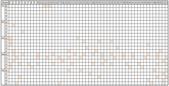
Figure 1. Scheduled maintenance tasks (in color).

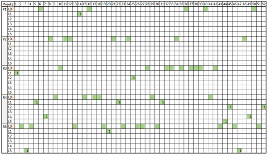
Figure 2. Maintenance tasks allocated to Crew Number 1 (in green color).

The first crew returns to the depot after performing a single task from the beginning until week seven. Furthermore, the crew stays at the depot for twelve weeks, between weeks thirty-two and forty-three. Similarly, work crew number two performs sixteen tasks. It is noticed that the tasks begin in the first and second week, followed by seven weeks at the depot before the next task is assigned. Following the completion of the task, there is a six-week period of stay at the depot. Unlike the concentrated weeks spent at the depot, the period of intense work spans from the twenty-eighth to the forty-third week, with only a few weeks spent at the depot during this time. Crew number three performs thirteen maintenance tasks. Initially, it carries out two consecutive tasks and then remains at the depot for eighteen weeks. Most of the work is executed without prolonged stays at the depot, taking place between week twenty-one and week thirty-nine. During this period, seven maintenance tasks are performed at regular intervals of one week, two weeks, or none. For crew number four, it has been observed that maintenance tasks are evenly distributed throughout the fifty-two weeks. The weeks, compared to the above-mentioned crews, remaining in the depot are fewer in aggregate over several weeks. The longest period in the depot is eight consecutive weeks and occurs in weeks twenty-nine to thirty-seven. The fifth crew is found to have the largest number of allocated tasks, equal to twenty-three. However, it is observed that sixteen of these tasks relate to the routine R4 and they are distributed approximately equally across all links. As a result, there can be optimal efficiency in completing the task R4, since this crew repeats the same task at regular intervals and thus knows the task requirements and communicates and collaborates better. Finally, the crew stays in the depot for twenty-nine weeks in total.

In addition, an essential result of the model is depicted in Figure 3, as it illustrates both the total scheduling of maintenance works and their allocation to different work crews. Thus, there is supervision of the work crews that will perform the tasks. There are a total of 82 scheduled tasks on the various links, out of which three are assigned to the project P1, two to the project P2, and the remaining are routine works, with 14 for R3, 47 for R4, and 16 for R5.

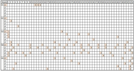
Figure 3. Scheduled maintenance tasks (in color) and crew allocations.

The seemingly high number of Routine R4 tasks is contingent on the frequency of tasks previously specified and validated based on the actual number of times they have been requested for execution. Similarly, the projects according to their possible starting time and duration in Table 3 are optimally allocated and verified. Project P1 has been executed with k= 1 in the twelfth to fourteenth week, P2 with k = 1 in the second week, and in the fifth week with k = 3. Furthermore, the pairs of combined tasks resulting in different links in the same week are: {[R3, R4], [P2, R3, R4], [R4, R5], [P2, R4], [P1, R4], [R3, R4, R5]}. According to the parameters we have defined, no task is performed on the same link simultaneously; rather, it is scheduled on different links, which helps to mitigate the track possession cost overhead. Additionally, the distribution of crews appears to be carefully planned, ensuring a balanced workload across all teams, and avoiding any undue burden on a particular crew. Finally, the scheduling of crew movements is optimized to minimize costs effectively.

In the following figures (Figure 4 and Figure 5), a comparison between the results of the baseline model [24] and our proposed model is illustrated. In the study of Budai and Dekker [24], only the first twenty weeks of planned maintenance tasks are given; thus, for comparison reasons, we have adjusted our results table based on the results from the baseline model. The numbering of routine works here is different, with {R1,R2,R3} routine works of the baseline model corresponding to {R3,R4,R5} in our model.

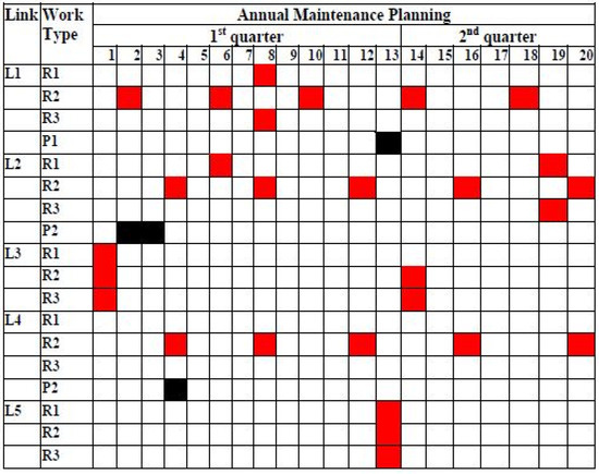
Figure 4. Annual maintenance planning—baseline model. Budai and Dekker [24].

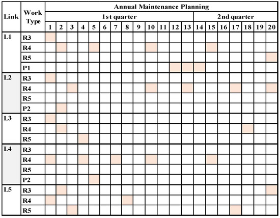
Figure 5. Annual maintenance planning—proposed model.

From the above figures, one can observe that most of the scheduled activities are planned for the link L1 in both approaches.

Overall, in comparison to the base model of Budai and Dekker [24], the objective function has been extended. This is the case since different values have been included for certain parameters, (e.g., duration of projects, pairs of combined tasks, scheduling period of routine tasks). To conduct a comparative analysis with the base model, our model was solved while excluding the work crews’ impact on the allocation of maintenance tasks. The objective was to maintain identical conditions to the base model, with only the modifications specific to our approach considered. The maintenance work’s total cost is EUR 8333, comprising EUR 8200 for track possession during each operation and EUR 133 for route cancellations and resource underutilization. In the base model, these costs were EUR 5700 and EUR 165, respectively. This variation from the implemented use case in this paper arises from the different combined pairs of tasks, which directly influence the track possession cost. Since more pairs of tasks cannot be simultaneously performed on the same link in this scenario, tasks are scheduled in other weeks, resulting in increased costs. The route cancellation cost, which has seen a slight reduction, is significantly influenced by the duration of projects taken at a different price compared to the base model. Additionally, the manner in which specific tasks are optimally performed also contributes to this cost. The model’s sensitivity to cost is crucial and highly relevant for railway operators. Simultaneously, the cost of work crews for executing the tasks is EUR 63,740, and this specific cost is weighted at 1 EUR per kilometer using the parameter in the $W_{lq}$ model. To sum up, maintenance tasks that included work crews in the objective function during the solution process resulted in varying execution times. This observation highlights that the model required the simultaneous optimization and scheduling of maintenance tasks and work crews to achieve the best outcomes.

Comparing our approach with additional studies, Lake et al. [29] presented a model designed to schedule track maintenance activities in the short term, once both the train schedule and maintenance plans have been established. The model’s primary aim is to arrange the maintenance tasks and allocate maintenance crews to them, all while striving to minimize the overall maintenance expenses. Furthemore, the formulation permitted the assignment of various crews to the same task at various moments and took into account the specific time needed for setting up and concluding each instance of the activity. The model was resolved through the implementation of a two-stage heuristic approach. In the first stage, a feasible solution was generated, and in the second stage, simulated annealing was employed. Our study further extends the aforementioned study, also including long-term maintenance activities (projects).

On the other hand, Buurman et al. [35] focused on optimizing the maintenance schedule for both railway operators and maintenance contractors considering hindrance and flexibility for both stakeholders. They formulated the problem as a multi-objective optimization problem (MOOP) with the first objective function minimizing the cost caused by hindrance for the train operators, and the second objective function maximizing the amount of scheduled slots in the maintenance schedule by maximizing the value of the maintenance slots above the maintenance demand. However, our research extends this study further by assigning a set of work crews to the maintenance tasks and minimizing their total costs.

6. Conclusions

The purpose of the present study was to introduce an optimization model designed for railway line preventive maintenance operations within a one-year timeframe. The aim was to enhance decision-making processes concerning railway line maintenance and the efficient allocation of work crews, ultimately leading to cost reduction. To achieve this, a mixed-binary linear mathematical program was developed and solved using the branch-and-cut algorithm of the GUROBI optimization software. While certain foundational elements of the model were based on existing input data, modifications and new data were incorporated. These additions pertained to the evolution of work crews in terms of integration with sets and parameters, as well as the necessary constraints to ensure functionality and adherence to requirements. Furthermore, variations were made to the baseline model of Budai and Dekker [24] that did not consider work crews, including frequency, duration, and task pairs, to analyze cost sensitivity. In the final step, a case study implementation was conducted, resulting in the annual maintenance schedules for tasks and work crews, along with the total cost of both. The results included concise maintenance scheduling tables to facilitate a comprehensive analysis of the model, evaluating its functionality and noting key observations. They revealed that consolidating tasks on the same link significantly reduced costs, and the workload was efficiently distributed among the work crews.

Finally, more comprehensive research should be pursued regarding the computation time limits of the search for an optimal solution, such as adding more tasks and exploring a larger network. Additionally, an investigation into the inclusion of train timetables to provide more precise task scheduling was deemed essential for further research. Lastly, testing scenarios with larger tasks would be beneficial to evaluate maintenance functionality and assess how costs are distributed in comparison to operators’ capabilities.

References

- Burgueño Salas, E. Rail Industry Worldwide—Statistics & Facts. Statista.com. 2022. Available online: https://www.statista.com/topics/1088/rail-industry/#topicOverview (accessed on 25 July 2023).
- Eurostat. Railway Passenger Transport Statistics—Quarterly and Annual Data. Eurostat—European Commission. 2022. Available online: https://ec.europa.eu/eurostat/statistics-explained/index.php?title=Railway_passenger_transport_statistics_-_quarterly_and_annual_data (accessed on 25 July 2023).
- Eurostat. Transport Statistics, 2018th ed.; Eurostat: Luxembourg, 2018. [Google Scholar]
- Rail Freight Forward. 30 By 2030—How Rail Freight Achieves Its Goals. 2020. Available online: https://www.railfreightforward.eu/ (accessed on 25 July 2023).
- EIM-EFRTC-CER Working Group. Market Strategies for Track Maintenance & Renewal. 2012, p. 53. Available online: http://www.cer.be/publications/brochures-studies-and-reports/report-eim-efrtc-cer-working-group-market-strategies (accessed on 25 July 2023).
- Kienzler, C.; Lotz, C.; Stern, S. Using Analytics to Get European Rail Maintenance on Track; McKinsey & Company: London, UK, 2021; pp. 1–11. [Google Scholar]
- Vale, C.; Ribeiro, I.M.; Calçada, R. Integer programming to optimize tamping in railway tracks as preventive maintenance. J. Transp. Eng. 2011, 138, 123–131. [Google Scholar] [CrossRef]
- Lidén, T. Survey of Railway Maintenance Activities from a Planning Perspective and Literature Review Concerning the use of Mathematical Algorithms for Solving Such Planning and Scheduling Problems; Linköpings Universitet: Norrköping, Sweden, 2014; p. 48. [Google Scholar]
- Lidén, T. Railway infrastructure maintenance—A survey of planning problems and conducted research. Transp. Res. Procedia 2015, 10, 574–583. [Google Scholar] [CrossRef]
- Dao, C.; Basten, R.; Hartmann, A. Maintenance Scheduling for Railway Tracks under Limited Possession Time. J. Transp. Eng. Part A Syst. 2018, 144, 1–9. [Google Scholar] [CrossRef]
- Vansteenwegen, P.; Dewilde, T.; Burggraeve, S.; Cattrysse, D. An iterative approach for reducing the impact of infrastructure maintenance on the performance of railway systems. Eur. J. Oper. Res. 2016, 252, 39–53. [Google Scholar] [CrossRef]
- Pour, S.M.; Drake, J.H.; Burke, E.K. A choice function hyper-heuristic framework for the allocation of maintenance tasks in Danish railways. Comput. Oper. Res. 2018, 93, 15–26. [Google Scholar] [CrossRef]
- Dotoli, M.; Epicoco, N.; Falagario, M.; Turchiano, B.; Cavone, G.; Convertini, A. A Decision Support System for real-time rescheduling of railways. In Proceedings of the 2014 European Control Conference (ECC), Strasbourg, France, 24–27 June 2014; pp. 696–701. [Google Scholar] [CrossRef]
- Sedghi, M.; Kauppila, O.; Bergquist, B.; Vanhatalo, E.; Kulahci, M. A taxonomy of railway track maintenance planning and scheduling: A review and research trends. Reliab. Eng. Syst. Saf. 2021, 215, 107827. [Google Scholar] [CrossRef]
- Cavone, G.; Van Den Boom, T.; Blenkers, L.; Dotoli, M.; Seatzu, C.; De Schutter, B. An MPC-Based Rescheduling Algorithm for Disruptions and Disturbances in Large-Scale Railway Networks. IEEE Trans. Autom. Sci. Eng. 2022, 19, 99–112. [Google Scholar] [CrossRef]
- Cavone, G.; Blenkers, L.; Van Den Boom, T.; Dotoli, M.; Seatzu, C.; De Schutter, B. Railway disruption: A bi-level rescheduling algorithm. In Proceedings of the 2019 6th International Conference on Control, Decision and Information Technologies (CoDIT), Paris, France, 23–26 April 2019; pp. 54–59. [Google Scholar] [CrossRef]
- Pour, S.M.; Drake, J.H.; Ejlertsen, L.S.; Rasmussen, K.M.; Burke, E.K. A hybrid Constraint Programming/Mixed Integer Programming framework for the preventive signaling maintenance crew scheduling problem. Eur. J. Oper. Res. 2018, 269, 341–352. [Google Scholar] [CrossRef]
- Pour, S.M.; Marjani Rasmussen, K.; Drake, J.H.; Burke, E.K. A constructive framework for the preventive signalling maintenance crew scheduling problem in the Danish railway system. J. Oper. Res. Soc. 2019, 70, 1965–1982. [Google Scholar] [CrossRef]
- Martinelli, D.R.; Teng, H. Optimization of Railway Operations Using Neural Networks. Transp. Res. Part C Emerg. Technol. 1996, 4, 33–49. [Google Scholar] [CrossRef]
- GENÇER, M.A.; YUMUŞAK, R.; ÖZCAN, E.; EREN, T. An Artificial Neural Network Model for Maintenance Planning of Metro Trains. Politek. Derg. 2021, 24, 811–820. [Google Scholar] [CrossRef]
- Popov, K.; De Bold, R.; Chai, H.K.; Forde, M.C.; Ho, C.L.; Hyslip, J.P.; Kashani, H.F.; Long, P.; Hsu, S.S. Big-data driven assessment of railway track and maintenance efficiency using Artificial Neural Networks. Constr. Build. Mater. 2022, 349, 128786. [Google Scholar] [CrossRef]
- Higgins, A. Scheduling of railway track maintenance activities and crews. J. Oper. Res. Soc. 1998, 49, 1026–1033. [Google Scholar] [CrossRef]
- Cheung, B.S.N.; Chow, K.P.; Hui, L.C.K.; Yong, A.M.K. Railway track possession assignment using constraint satisfaction. Eng. Appl. Artif. Intell. 1999, 12, 599–611. [Google Scholar] [CrossRef]
- Budai, G.; Dekker, R. A dynamic approach for planning preventive railway maintenance activities. Adv. Transp. 2004, 15, 323–332. [Google Scholar]
- Budai, G.; Huisman, D.; Dekker, R. Scheduling preventive railway maintenance activities. J. Oper. Res. Soc. 2006, 57, 1035–1044. [Google Scholar] [CrossRef]
- Peng, F.; Ouyang, Y. Track maintenance production team scheduling in railroad networks. Transp. Res. Part B Methodol. 2012, 46, 1474–1488. [Google Scholar] [CrossRef]
- Heinicke, F.; Simroth, A.; Scheithauer, G.; Fischer, A. A railway maintenance scheduling problem with customer costs. EURO J. Transp. Logist. 2015, 4, 113–137. [Google Scholar] [CrossRef]
- Van Zante-De Fokkert, J.I.; Den Hertog, D.; Van Den Berg, F.J.; Verhoeven, J.H.M. The Netherlands schedules track maintenance to improve track workers’ safety. Interfaces 2007, 37, 133–142. [Google Scholar] [CrossRef]
- Lake, M.; Ferreira, L.; Murray, M. Minimising costs in scheduling railway track maintenance. Adv. Transp. 2000, 7, 895–902. [Google Scholar]
- Den Hertog, D.; Van Zante-De Fokkert, J.I.; Sjamaar, S.A.; Beusmans, R. Optimal working zone division for safe track maintenance in the Netherlands. Accid. Anal. Prev. 2005, 37, 890–893. [Google Scholar] [CrossRef]
- Andrade, A.R.; Teixeira, P.F. Biobjective optimization model for maintenance and renewal decisions related to rail track geometry. Transp. Res. Rec. 2011, 2261, 163–170. [Google Scholar] [CrossRef]
- Su, Z.; Jamshidi, A.; Núñez, A.; Baldi, S.; De Schutter, B. Integrated condition-based track maintenance planning and crew scheduling of railway networks. Transp. Res. Part C Emerg. Technol. 2019, 105, 359–384. [Google Scholar] [CrossRef]
- Nijland, F.; Gkiotsalitis, K.; van Berkum, E.C. Improving railway maintenance schedules by considering hindrance and capacity constraints. Transp. Res. Part C Emerg. Technol. 2021, 126, 103108. [Google Scholar] [CrossRef]
- Oudshoorn, M.; Koppenberg, T.; Yorke-Smith, N. Optimization of annual planned rail maintenance. Comput. Civ. Infrastruct. Eng. 2022, 37, 669–687. [Google Scholar] [CrossRef]
- Buurman, B.; Gkiotsalitis, K.; van Berkum, E.C. Railway maintenance reservation scheduling considering detouring delays and maintenance demand. J. Rail Transp. Plan. Manag. 2023, 25, 100359. [Google Scholar] [CrossRef]
- Bueno, P.M.S.; Vilela, P.R.S.; Christofoletti, L.M.; Vieira, A.P. Optimizing railway track maintenance scheduling to minimize circulation impacts. In Proceedings of the 2019 Joint Rail Conference, Snowbird, UT, USA, 9–12 April 2019. [Google Scholar]
- Lidén, T.; Joborn, M. An optimization model for integrated planning of railway traffic and network maintenance. Transp. Res. Part C Emerg. Technol. 2017, 74, 327–347. [Google Scholar] [CrossRef]
- D’Ariano, A.; Meng, L.; Centulio, G.; Corman, F. Integrated stochastic optimization approaches for tactical scheduling of trains and railway infrastructure maintenance. Comput. Ind. Eng. 2019, 127, 1315–1335. [Google Scholar] [CrossRef]
- Albrecht, A.R.; Panton, D.M.; Lee, D.H. Rescheduling rail networks with maintenance disruptions using Problem Space Search. Comput. Oper. Res. 2013, 40, 703–712. [Google Scholar] [CrossRef]
- Forsgren, M.; Aronsson, M.; Gestrelius, S. Maintaining tracks and traffic flow at the same time. J. Rail Transp. Plan. Manag. 2013, 3, 111–123. [Google Scholar] [CrossRef]
Disclaimer/Publisher’s Note: The statements, opinions and data contained in all publications are solely those of the individual author(s) and contributor(s) and not of MDPI and/or the editor(s). MDPI and/or the editor(s) disclaim responsibility for any injury to people or property resulting from any ideas, methods, instructions or products referred to in the content. |
© 2023 by the authors. Licensee MDPI, Basel, Switzerland. This article is an open access article distributed under the terms and conditions of the Creative Commons Attribution (CC BY) license (https://creativecommons.org/licenses/by/4.0/).