Weighted Group Sparse Regularized Tensor Decomposition for Hyperspectral Image Denoising

Abstract

Hyperspectral imaging (HSI) has been used in a wide range of applications in recent years. But in the process of image acquisition, hyperspectral images are subject to various types of noise interference. Noise reduction algorithms can be used to enhance the quality of images and make it easier to detect and analyze features of interest. To realize better image recovery, we propose a weighted group sparsity-regularized low-rank tensor ring decomposition (LRTRDGS) method for hyperspectral image recovery. Tensor ring decomposition can be utilized by this approach to investigate self-similarity and global spectral correlation. Furthermore, weighted group sparsity regularization can be employed to depict the sparsity structure of the group along the spectral dimension of the spatial difference image. Moreover, we solve the proposed model using a symmetric alternating direction method multiplier with the addition of a proximity term. The experimental data verify the effectiveness of our proposed method.

1. Introduction

Hyperspectral imaging (HSI) is a powerful tool for studying and analyzing data for various applications. HSI uses a combination of visible, infrared and ultraviolet wavelengths to capture images in a way that traditional imaging methods cannot. HSI manifests two essential attributes: spatial and spectral resolutions. Specifically, it possesses two spatial dimensions and one spectral dimension. As a result, it generates an almost uninterrupted reflectance spectrum for each pixel within the scene. This, in turn, facilitates a comprehensive spectral analysis of scene attributes that would otherwise prove challenging to identify using a broader range of multispectral scanners [1]. The Flying Laboratory of Imaging Systems (FLIS) provides a single platform that combines hyperspectral, thermal and laser scanning to produce high-quality remote sensing data [2].

HSI has many applications, such as mining [3], analyzing crops in agriculture [4,5], astroplanetary exploration [6], medical images [7], mineral exploration [8], the detection of soil-borne viruses [9] and the measurement of water quality [10]. High-spectral-resolution images often contain noise, which can significantly reduce their performance and accuracy. Hence, attenuating noise holds great significance in scrutinizing high-spectral-resolution pictures. This technique aids in augmenting image quality, thereby facilitating the identification and examination of intriguing attributes. With noise reduction algorithms, HSI is more useful and accurate for various applications.

Tensor is a powerful mathematical tool for extracting information from HSI images. It allows us to see patterns and relationships between different parts of an image that are not visible with traditional imaging techniques, and it is possible to analyze and interpret the data in a much more sophisticated way. Many experts use tensor methods, such as Tucker decomposition [11,12], canonical polyadic (CP) decomposition [13,14] and tensor singular-value decomposition (t-SVD) [15] for hyperspectral image analysis. For example, a model for the weighted group of low-rank tensor decomposition with regularized sparsity (LRTDGS) based on Tucker decomposition was proposed by Chen et al. [16]. Using Tucker decomposition, Wang et al. developed a hybrid noise removal method for HSI [17]. In their study, Zhao et al. introduced a nonlocal low-rank regularized canonical polyadic tensor decomposition method (NLR-CPTD) that relies on two prior information sources: GCS and nonlocal self-similarity [18]. The weighted Schatten $l_p$-norm low-rank matrix approximation (WSN-LRMA) method was developed by Xie et al. In this method, the eigenvalues were obtained through t-SVD [19]. Despite the satisfactory denoising results obtained through the aforementioned techniques, there is still significant potential for enhancing the efficiency of denoising hyperspectral images.

Many scholars have recently proposed a decomposition method based on tensor rings (TRs) using cyclically contracted third-order tensors to represent higher-order tensors [20,21]. Circular shifting and equivalence can be performed according to the tensor ring factor, which can effectively balance the correlation between the modes. TR decomposition can better approximate higher-order tensors. For tensor completion, refs. [22,23] verified that the TR method obtains better results than the Tucker and CP decomposition methods. TR is able to improve accuracy and enhance security. It can store and process data with greater accuracy than traditional methods, as the three-dimensional structure of the ring allows for a more precise representation of the data. This improved accuracy helps to ensure accuracy during data processing. Data stored in a tensor ring are more secure than data processed by traditional methods, as the three-dimensional structure of the ring makes it difficult to hack or access the data without authorization. This means that data stored in a tensor ring are more secure than data stored in stationary locations.

The total variational (TV) regularization method was first proposed by Rudin et al. [24]. This technology effectively preserves the spatial sparsity and smoothness of images, making it applicable in various image processing tasks, like denoising, magnetic resonance and superresolution. He et al. proposed total variational regularized low-rank matrix decomposition (LRTV) [25]. Wang et al. proposed a spectral–spatial total variational regularization (SSTV) method to construct a smooth structure in the spectral and spatial domains [17]. He et al. also presented the method of local low-rank matrix recovery, known as spatial–spectral total variance regularization (LLRSSTV), which aims to effectively exploit the total variance nature of the variance in each direction of hyperspectral images for reorganizing the local low-rank patches [26]. However, most of the methods utilize one-norm constraints on the spatial difference images to promote structural segmentation smoothing. To address the issue of the ineffective depiction of the group sparse structure within the spectral dimensional spatial difference image, Chen et al. introduced a novel approach for hyperspectral image recovery. This technique employs weighted group sparsity-regularized low-rank tensor decomposition to overcome the limitation of the one-norm [16].

In light of the preceding discussion, we present a novel approach for enhancing hyperspectral image quality through the utilization of weighted group sparsity-regularized low-rank tensor ring decomposition (LRTRDGS). The method combines the advantages of tensor ring decomposition and weighted group sparse regularization. A symmetric alternating direction of multipliers method with a proximity point operator is used to solve our proposed model. This paper focuses on the following main topics:

(1)

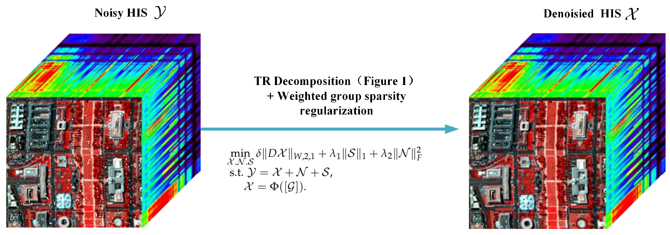
Utilizing the global spatial and spectral correlation among hyperspectral images, the tensor ring decomposition technique is employed to segregate unpolluted hyperspectral images from raw observations that have been tainted with intricate noise.

(2)

Due to the fact that the gradient components in smooth areas of hyperspectral images typically exhibit a complete absence (a value of zero) in the spectral dimension, the gradient components in edge regions demonstrate non-zero values. Hence, to address this discrepancy, we incorporate a regularization term, with the group sparsity weighted, into the framework of tensor ring decomposition. It can explore the group structure of spatially differential images along the spectral dimension.

(3)

A symmetric alternating direction method multiplier is employed to solve the model of the low-rank tensor ring decomposition with regularization on weighted group sparsity. To enhance the efficiency of this method, a proximity point operator is incorporated. Through numerical experiments, it has been determined that this approach outperforms other commonly utilized methods in terms of both quantitative evaluation and visual comparison.

The structure of this paper is as follows. Several notations are presented, and the tensor ring is defined in Section 2. Section 3 proposes a hyperspectral image denoising model based on weighted group sparse regularized tensor ring decomposition and presents the model solving method. In Section 4, we present the experimental results for the simulated data and discuss the parametric analysis and convergence analysis. We summarize the proposed method in Section 5.

2. Notations and Tensor Ring

This section describes the notations used throughout this paper and introduces the tensor ring approach presented in [20].

2.1. Notations

Following the nomenclature in [27], we summarize the notations used in this paper as follows. x is a scalar, $\mathbf{x}$ is a vector, $\mathbf{X}$ is a matrix and $\mathcal{X}$ is a tensor. $x_{i_1,i_2,\dots ,i_N}$ or $\mathbf{X}(i_1,i_2,\dots ,i_N)$ is the $(i_1,i_2,\dots ,i_N)$th element of $\mathcal{X}$. ${\mathbf{x}}_{:,i_2,i_3}$ or $\mathcal{X}(:,i_2,i_3)$ is the $(i_2,i_3)$th column of a third-order tensor $\mathcal{X}$. ${\mathbf{x}}_{i_1,:,i_3}$ or $\mathcal{X}(i_1,:,i_3)$ is the $(i_1,i_3)$th row of a third-order tensor $\mathcal{X}$. ${\mathbf{x}}_{i_1,i_2,:}$ or $\mathcal{X}(i_1,i_2,:)$ is the $(i_1,i_2)$th tubal of a third-order tensor $\mathcal{X}$. ${\parallel \mathcal{X}\parallel }_F=\sqrt{{\Sigma }_{i_1,i_2,\dots ,i_N}{\left|x_{i_1,i_2,\dots ,i_N}\right|}^2}$ is the Frobenius norm. ${\parallel \mathcal{X}\parallel }_1={\Sigma }_{i_1,i_2,\dots ,i_N}\left|x_{i_1,i_2,\dots ,i_N}\right|$ is the $l_1$-norm. ${\mathbf{X}}_{\left(k\right)}$ is the mode-k unfolding of $\mathcal{X}$. $<·,·>$ is the inner product. ⨂ is the Kronecker product. ⨀ is componentwise multiplication. ${\times }_k$ is the mode-k tensor matrix product.

In order to increase the readability of this article, we summarize the abbreviations of the names in Abbreviations part.

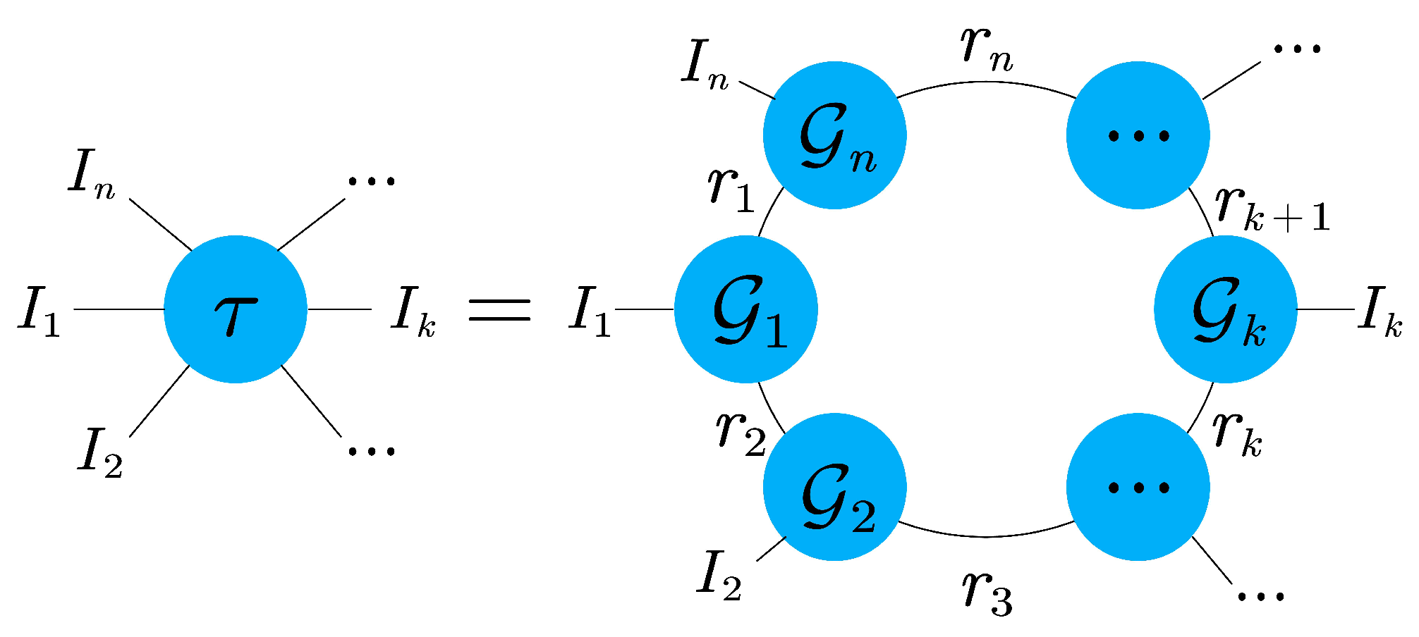
2.2. Tensor Ring

In this segment, we present the technique of the tensor ring and the corresponding definitions linked to it. The tensor ring structure is a superior and effective form of decomposition in comparison to other types of tensor decomposition. TR decomposition can be represented as a sequence of cyclic multiplicative third-order tensors with a higher-order tensor. The nth-tensor is denoted as $\mathcal{X}\in {\mathbb{R}}^{I_1\times \dots \times I_n}$. The representation of the tensor ring can be decomposed into a series of latent tensors,

$$\begin{array}{c}\mathcal{X}(i_1,i_2,\dots ,i_n)=Tr\{{\mathbf{G}}_1\left(i_1\right){\mathbf{G}}_2\left(i_2\right)\dots {\mathbf{G}}_n\left(i_n\right)\}\hfill \\ =Tr\left\{{\displaystyle \prod _{k=1}^n}{\mathbf{G}}_k\left(i_k\right)\right\}\hfill \end{array}$$

(1)

where $\mathcal{X}(i_1,i_2,\dots ,i_n)$ is the $(i_1,i_2,\dots ,i_n)$th element of the tensor. ${\mathbf{G}}_k\left(i_k\right)$ represents the $i_k$th lateral slice matrix of the latent tensor ${\mathcal{G}}_k$. It has a size of $r_k\times r_{k+1}$. Any two adjacent latent tensors ${\mathcal{G}}_k$ and ${\mathcal{G}}_{k+1}$ have equivalent dimensions of $r_{k+1}$ on their corresponding modes. The last latent tensor ${\mathcal{G}}_n$ has a size of $r_n\times I_n\times r_1$, i.e., $r_{n+1}=r_1$, which ensures that the product of these matrices is a square matrix. In some cases, the latent tensor ${\mathcal{G}}_k$ is called the kth-core. $r_k(k=1,2,\dots ,n)$ is the size of the cores. $\mathbf{r}=[r_1,r_2,\dots ,r_n]$ are known as TR ranks. According to (1), the trace of a sequential product of matrices $\left\{{\mathbf{G}}_k\left(i_k\right)\right\}$ is equivalent to $\mathcal{X}(i_1,i_2,\dots ,i_n)$. In addition, (1) can be rewritten as follows:

$$\begin{array}{c}\mathcal{X}(i_1,i_2,\dots ,i_n)={\displaystyle \sum _{{\alpha }_1,\dots ,{\alpha }_n=1}^{r_1,\dots ,r_n}}{\displaystyle \prod _{k=1}^n}{G}_k({\alpha }_k,i_k,{\alpha }_{k+1}).\hfill \end{array}$$

(2)

where k represents the tensor modes, $i_k$ represents the data dimension index and ${\alpha }_k$ represents the latent dimension index. For $\forall k\in \{1,\dots ,n\}$, $1\le {\alpha }_k\le r_k$, $1\le i_k\le I_k$, Equation (2) can also be written as follows:

$$\begin{array}{c}\mathcal{X}={\displaystyle \sum _{{\alpha }_1,\dots ,{\alpha }_n=1}^{r_1,\dots ,r_n}}{\mathbf{g}}_1({\alpha }_1,{\alpha }_2)\circ {\mathbf{g}}_2({\alpha }_2,{\alpha }_3)\circ \dots \circ {\mathbf{g}}_n({\alpha }_n,{\alpha }_1).\hfill \end{array}$$

(3)

where ‘∘’ is the outer product of the vector. ${\mathbf{g}}_k({\alpha }_k,{\alpha }_{k+1})\in {\mathbb{R}}^{I_k}$ is the $({\alpha }_k,{\alpha }_{k+1})$ mode-2 fiber of tensor $\mathcal{X}$.

Figure 1 graphically represents the tensor ring using a linear tensor network. The order of each tensor is determined by its edges, with every node representing a tensor. The size of each mode is indicated by the number on the corresponding edge. The tensor contraction, also known as the multilinear product operator, occurs when two tensors are connected on a specific mode. For a more comprehensive explanation, please refer to the provided reference [20].

Figure 1. A graphical representation of tensor ring decomposition.

Definition 1.

(Multilinear Product). For the two adjacent cores of TR decomposition ${\mathcal{G}}_k$ and ${\mathcal{G}}_{k+1}$, ${\mathcal{G}}_{k,k+1}\in {\mathbb{R}}^{r_k\times I_k{I}_{k+1}\times r_{k+1}}$ is the multilinear product of the two cores:

$$\begin{array}{c}{\mathcal{G}}_{k,k+1}(I_n(i_k-1)+j_k)={\mathcal{G}}_k\left(i_k\right){\mathcal{G}}_{k+1}\left(j_k\right).\hfill \end{array}$$

(4)

where $i_k=1,\dots ,I_k,j_k=1,\dots ,I_{k+1}$.

According to Definition 1, it is established that the tensor $\mathcal{X}$ can be expressed as the multilinear outcome of a series of core tensors of the third order, known as TR decomposition, i.e.,

$$\begin{array}{c}\mathcal{X}=\Phi \left(\right[\mathcal{G}\left]\right),\hfill \end{array}$$

(5)

where $\Phi$ is the reconfiguration operator of TR and $\left[\mathcal{G}\right]={\displaystyle \prod _{k=1}^n}{\mathcal{G}}_k=\{{\mathcal{G}}_1,{\mathcal{G}}_2,\dots ,{\mathcal{G}}_n\}$.

3. Proposed Method

Assuming that the noise is independent in the denoising problem, we usually consider the following degradation model:

$$\mathcal{Y}=\mathcal{X}+\mathcal{S}+\mathcal{N},$$

(6)

where $\mathcal{X}\in {\mathbb{R}}^{I_1\times I_2\times I_3}$ is the clean hyperspectral image; $\mathcal{N}\in {\mathbb{R}}^{I_1\times I_2\times I_3}$ is Gaussian noise; $\mathcal{S}\in {\mathbb{R}}^{I_1\times I_2\times I_3}$ is sparse noise; $I_1\times I_2$ is the hyperspectral images spatial size; and $I_3$ is the number of bands in the spectral analysis.

Based on this degradation model, we propose LRTRDGS, which is recovered by tensor ring constraints and preserves fine details by group sparse regularization. The framework of the proposed LRTRDGS method is depicted in Figure 2. The LRTRDGS model is represented as follows:

$$\begin{array}{c}\underset{\mathcal{X}.\mathcal{N}.\mathcal{S}}{\min }{\delta \parallel D\mathcal{X}\parallel }_{W,2,1}+{\lambda }_1{\parallel \mathcal{S}\parallel }_1+{\lambda }_2{\parallel \mathcal{N}\parallel }_F^2\hfill \\ \mathrm{s}.\mathrm{t}.\mathcal{Y}=\mathcal{X}+\mathcal{N}+\mathcal{S},\hfill \\ \mathcal{X}=\Phi \left(\right[\mathcal{G}\left]\right).\hfill \end{array}$$

(7)

where D is composed of $D_x$ and $D_y$, which are two differential operators in two spatial dimensions. The weighted $l_{2,1}$-norm of $D\mathcal{X}$ is as follows:

$${\parallel D\mathcal{X}\parallel }_{W,2,1}=\sum _{i=1}^m\sum _{j=1}^n{W}_x(i,j)\parallel D_x{\mathcal{X}(i,j,:)\parallel }_2+\sum _{i=1}^m\sum _{j=1}^n{W}_y(i,j){\parallel D_y\mathcal{X}(i,j,:)\parallel }_2.$$

Figure 2. Framework of the proposed HSI denoising method.

To solve the LRTRDGS model (7), we propose a symmetric alternating direction method of the multiplier (ADMM) that incorporates proximity point operators. In the upcoming phases, the suggested ADMM will be implemented to address the proposed model. Two auxiliary variables can be introduced to the model (7) and are expressed as follows:

$$\begin{array}{c}\underset{\mathcal{X}.\mathcal{N}.\mathcal{S}}{\min }{\delta \parallel \mathcal{P}\parallel }_{W,2,1}+{\lambda }_1{\parallel \mathcal{S}\parallel }_1+{\lambda }_2{\parallel \mathcal{N}\parallel }_F^2\hfill \\ \mathrm{s}.\mathrm{t}.\mathcal{Y}=\mathcal{X}+\mathcal{N}+\mathcal{S},\hfill \\ \mathcal{X}=\mathcal{Q},\mathcal{P}=D\mathcal{Q},\hfill \\ \mathcal{X}=\Phi \left(\right[\mathcal{G}\left]\right).\hfill \end{array}$$

(8)

Under the constraint of tensor ring decomposition $\mathcal{X}=\Phi \left(\right[\mathcal{G}\left]\right)$, this problem has the following augmented Lagrangian function:

$$\begin{array}{c}{L}_{\mu }\left(\mathcal{X},\mathcal{S},\mathcal{N},\mathcal{P},\mathcal{Q},{\Lambda }_1,{\Lambda }_2,{\Lambda }_3\right)={\delta \parallel \mathcal{P}\parallel }_{W,2,1}+{\lambda }_1{\parallel \mathcal{S}\parallel }_1+{\lambda }_2{\parallel \mathcal{N}\parallel }_F^2+⟨{\Lambda }_1,\mathcal{Y}-\mathcal{X}-\mathcal{N}-\mathcal{S}⟩\hfill \\ +⟨{\Lambda }_2,\mathcal{X}-\mathcal{Q}⟩+⟨{\Lambda }_3,D\mathcal{Q}-\mathcal{P}⟩+\frac{\mu }{2}\left({\parallel \mathcal{Y}-\mathcal{X}-\mathcal{N}-\mathcal{S}\parallel }_F^2{+\parallel \mathcal{X}-\mathcal{Q}\parallel }_F^2+{\parallel D\mathcal{Q}-\mathcal{P}\parallel }_F^2\right),\hfill \end{array}$$

(9)

where ${\Lambda }_1$, ${\Lambda }_2$ and ${\Lambda }_3$ are the Lagrange multipliers and $\mu$ is a positive scalar. As seen from the Lagrangian function, all variables are independent. We fix other variables and choose suitable ones to optimize the incremental Lagrangian function in (9). To optimize the incremental Lagrangian function in (9), we need to fix the other variables and select the appropriate ones. In addition, we make use of the symmetric ADMM with the addition of the proximity point operator to improve the convergence speed of the algorithm. The specific algorithm framework is as follows:

$$\left\{\begin{array}{c}{\mathcal{X}}^{p+1}=\underset{\mathcal{X}}{\arg \min }{\mathcal{L}}_{\mu }\left(\mathcal{X},{\mathcal{S}}^p,{\mathcal{N}}^p,{\mathcal{P}}^p,{\mathcal{Q}}^p,{\Lambda }_1^p,{\Lambda }_2^p,{\Lambda }_3^p\right)\hfill \\ {\Lambda }_1^{p+\frac{1}{2}}={\Lambda }_1^p+v_1\mu \left(\mathcal{Y}-{\mathcal{X}}^{p+1}-{\mathcal{N}}^p-{\mathcal{S}}^p\right)\hfill \\ {\Lambda }_2^{p+\frac{1}{2}}={\Lambda }_2^p+v_2\mu \left({\mathcal{X}}^{p+1}-{\mathcal{Q}}^p\right)\hfill \\ {\mathcal{Q}}^{p+1}=\underset{\mathcal{Q}}{\arg \min }{\mathcal{L}}_{\mu }\left({\mathcal{X}}^{p+1},{\mathcal{S}}^p,{\mathcal{N}}^p,{\mathcal{P}}^p,\mathcal{Q},{\Lambda }_1^{p+\frac{1}{2}},{\Lambda }_2^{p+\frac{1}{2}},{\Lambda }_3^p\right)+\frac{\sigma \mu }{2}{\parallel \mathcal{Q}-{\mathcal{Q}}^p\parallel }_F^2\hfill \\ {\Lambda }_3^{p+\frac{1}{2}}={\Lambda }_3^p+v_3\mu \left(D{\mathcal{Q}}^{p+1}-{\mathcal{P}}^p\right)\hfill \\ {\mathcal{P}}^{p+1}=\underset{\mathcal{P}}{\arg \min }{\mathcal{L}}_{\mu }\left({\mathcal{X}}^{p+1},{\mathcal{S}}^p,{\mathcal{N}}^p,\mathcal{P},{\mathcal{Q}}^{p+1},{\Lambda }_1^{p+\frac{1}{2}},{\Lambda }_2^{p+\frac{1}{2}},{\Lambda }_3^{p+\frac{1}{2}}\right)\hfill \\ {\mathcal{S}}^{p+1}=\underset{\mathcal{S}}{\arg \min }{\mathcal{L}}_{\mu }\left({\mathcal{X}}^{p+1},\mathcal{S},{\mathcal{N}}^p,{\mathcal{P}}^{p+1},{\mathcal{Q}}^{p+1},{\Lambda }_1^{p+\frac{1}{2}},{\Lambda }_2^{p+\frac{1}{2}},{\Lambda }_3^{p+\frac{1}{2}}\right)\hfill \\ {\mathcal{N}}^{p+1}=\underset{\mathcal{N}}{\arg \min }{\mathcal{L}}_{\mu }\left({\mathcal{X}}^{p+1},{\mathcal{S}}^{p+1},\mathcal{N},{\mathcal{P}}^{p+1},{\mathcal{Q}}^{p+1},{\Lambda }_1^{p+\frac{1}{2}},{\Lambda }_2^{p+\frac{1}{2}},{\Lambda }_3^{p+\frac{1}{2}}\right)\hfill \\ {\Lambda }_1^{p+1}={\Lambda }_1^{p+\frac{1}{2}}+v_4\mu \left(\mathcal{Y}-{\mathcal{X}}^{p+1}-{\mathcal{N}}^{p+1}-{\mathcal{S}}^{p+1}\right)\hfill \\ {\Lambda }_2^{p+1}={\Lambda }_2^{p+\frac{1}{2}}+v_5\mu \left({\mathcal{X}}^{p+1}-{\mathcal{Q}}^{p+1}\right)\hfill \\ {\Lambda }_3^{p+1}={\Lambda }_3^{p+\frac{1}{2}}+v_6\mu \left(D{\mathcal{Q}}^{p+1}-{\mathcal{P}}^{p+1}\right)\hfill \end{array}\right.$$

(10)

In the $p+1$th iteration, we update the variables involved in model (10) as follows:

(1) Subproblem $\mathcal{X}$:

$$\begin{array}{c}{\displaystyle \underset{\mathcal{X}=\Phi \left(\right[\mathcal{G}\left]\right)}{\min }}⟨{\Lambda }_1^p,\mathcal{Y}-\mathcal{X}-{\mathcal{N}}^p-{\mathcal{S}}^p⟩+⟨{\Lambda }_2^p,\mathcal{X}-{\mathcal{Q}}^p⟩+\frac{\mu }{2}\left(\parallel \mathcal{Y}-\mathcal{X}-{\mathcal{N}}^p-{\mathcal{S}}^p{\parallel }_F^2+{\parallel \mathcal{X}-{\mathcal{Q}}^p\parallel }_F^2\right)\hfill \end{array}$$

(11)

(11) can be expressed as

$$\begin{array}{c}\min \mu \parallel \Phi \left(\left[\mathcal{G}\right]\right)-\frac{1}{2}\left(\mathcal{Y}-{\mathcal{N}}^p-{\mathcal{S}}^p+{\mathcal{Q}}^p+\left({\Lambda }_1^p-{\Lambda }_2^p\right)/\mu \right){\parallel }_F^2\hfill \end{array}$$

(12)

Through tensor ring decomposition, we can easily obtain ${\mathcal{G}}^{p+1}$, and $\mathcal{X}$ can be updated as follows:

$$\begin{array}{c}{\mathcal{X}}^{p+1}=\Phi \left(\left[{\mathcal{G}}^{p+1}\right]\right).\hfill \end{array}$$

(13)

(2) Subproblem $\mathcal{Q}$:

$$\begin{array}{c}{\mathcal{Q}}^{p+1}=\arg \underset{\mathcal{Q}}{\min }⟨{\Lambda }_2^{p+\frac{1}{2}},{\mathcal{X}}^{p+1}-\mathcal{Q}⟩+⟨{\Lambda }_3^p,D\mathcal{Q}-{\mathcal{P}}^p⟩\hfill \\ +\frac{\mu }{2}\left(\parallel {\mathcal{X}}^{p+1}{-\mathcal{Q}\parallel }_F^2+{\parallel D\mathcal{Q}-{\mathcal{P}}^p\parallel }_F^2\right)+\frac{\sigma \mu }{2}{\parallel \mathcal{Q}-{\mathcal{Q}}^p\parallel }_F^2\hfill \end{array}$$

(14)

This problem can be optimized with the following linear system:

$$\begin{array}{c}\left(\mu I+\mu D^{*}D+\sigma \mu \right)\mathcal{Q}=\mu {\mathcal{X}}^{p+1}+\mu D^{*}\left({\mathcal{P}}^p\right)+{\Lambda }_2^{p+\frac{1}{2}}-D^{*}\left({\Lambda }_3^p\right)+\sigma \mu {\mathcal{Q}}^p\hfill \end{array}$$

where $D^{*}$ is the adjoint operator of D. The matrix corresponding to operator $D^{*}D$ has a block cycle structure, which can be diagonalized by the 3-D Fast Fourier Transform (FFT) matrix. Thus, we have

$$\left\{\begin{array}{c}{H}_{\mathcal{Q}}=\mu {\mathcal{X}}^{p+1}+\mu D^{*}\left({\mathcal{P}}^p\right)+{\Lambda }_2^{p+\frac{1}{2}}-D^{*}\left({\Lambda }_3^p\right)+\sigma \mu {\mathcal{Q}}^p,\hfill \\ T_{\mathcal{Q}}=W_x^2|fftn\left(D_x\right){|}^2+W_y^2{\left|fftn\left(D_y\right)\right|}^2,\hfill \\ {\mathcal{Q}}^{p+1}=ifftn\left(\frac{fftn\left(H_{\mathcal{Q}}\right)}{\mu I+\mu T_{\mathcal{Q}}+\sigma \mu }\right)\hfill \end{array}\right.$$

(15)

where $fftn$ and $ifftn$ correspond to the rapid 3-D Fourier transformation and its inverse conversion, respectively. The squared component is denoted by ${|·|}^2$, with division being executed in an element-wise manner.

(3) Subproblem $\mathcal{P}$:

$$\begin{array}{c}{\mathcal{P}}^{p+1}=\arg \underset{\mathcal{P}}{\min }{\delta \parallel \mathcal{P}\parallel }_{W,2,1}+⟨{\Lambda }_3^{p+\frac{1}{2}},D{\mathcal{Q}}^{p+1}-\mathcal{P}⟩+\frac{\mu }{2}{\parallel D{\mathcal{Q}}^{p+1}-\mathcal{P}\parallel }_F^2\hfill \\ =\arg \underset{\mathcal{P}}{\min }{\delta \parallel \mathcal{P}\parallel }_{W,2,1}+\frac{\mu }{2}\parallel \mathcal{P}-\left(D{\mathcal{Q}}^{p+1}+\frac{{\Lambda }_3^{p+\frac{1}{2}}}{\mu }\right){\parallel }_F^2.\hfill \end{array}$$

(16)

Using the soft threshold operator,

$$R_{\Delta }\left(\mathbf{x}\right)=\left\{\begin{array}{cc}x-\Delta ,\hfill & if\mathbf{x}>\Delta \hfill \\ x+\Delta ,\hfill & if\mathbf{x}<\Delta \hfill \\ 0,\hfill & otherwise\hfill \end{array}\right.$$

where $x\in \mathbb{R}$, and $\Delta >0$, we have:

$$\begin{array}{c}{\mathcal{P}}^{p+1}=R_{\frac{\delta }{\mu }}\left(D{\mathcal{Q}}^{p+1}+\frac{{\Lambda }_3^{p+\frac{1}{2}}}{\mu }\right).\hfill \end{array}$$

(17)

(4) Subproblem $\mathcal{S}$:

$$\begin{array}{c}{\mathcal{S}}^{p+1}=\arg \underset{\mathcal{S}}{\min }{\lambda }_1{\parallel \mathcal{S}\parallel }_1+⟨{\Lambda }_1^{p+\frac{1}{2}},\mathcal{Y}-{\mathcal{X}}^{p+1}-{\mathcal{N}}^p-\mathcal{S}⟩+\frac{\mu }{2}{\parallel \mathcal{Y}-{\mathcal{X}}^{p+1}-{\mathcal{N}}^p-\mathcal{S}\parallel }_F^2\hfill \\ =\arg \underset{\mathcal{S}}{\min }{\lambda }_1{\parallel \mathcal{S}\parallel }_1+\frac{\mu }{2}\parallel \mathcal{Y}-{\mathcal{X}}^{p+1}-{\mathcal{N}}^p-\mathcal{S}+\frac{{\Lambda }_1^{p+\frac{1}{2}}}{\mu }{\parallel }_F^2\hfill \end{array}$$

(18)

By applying the aforementioned soft threshold operator, one can acquire the solution to the described problem:

$$\begin{array}{c}{\mathcal{S}}^{p+1}=R_{\frac{{\lambda }_1}{\mu }}\left(\mathcal{Y}-{\mathcal{X}}^{p+1}-{\mathcal{N}}^p+\frac{{\Lambda }_1^{p+\frac{1}{2}}}{\mu }\right).\hfill \end{array}$$

(19)

(5) Subproblem $\mathcal{N}$:

$$\begin{array}{c}{\mathcal{N}}^{p+1}=\arg \underset{\mathcal{N}}{\min }{\lambda }_2{\parallel \mathcal{N}\parallel }_F^2+⟨{\Lambda }_1^{p+\frac{1}{2}},\mathcal{Y}-{\mathcal{X}}^{p+1}-\mathcal{N}-{\mathcal{S}}^{p+1}⟩+\frac{\mu }{2}{\parallel \mathcal{Y}-{\mathcal{X}}^{p+1}-{\mathcal{S}}^{p+1}-\mathcal{N}\parallel }_F^2\hfill \\ =\arg \underset{\mathcal{N}}{\min }\left({\lambda }_2+\frac{\mu }{2}\right)\parallel \mathcal{N}-\frac{\mu \left(\mathcal{Y}-{\mathcal{X}}^{p+1}-{\mathcal{S}}^{p+1}\right)+{\Lambda }_1^{p+\frac{1}{2}}}{\mu +2{\lambda }_2}{\parallel }_F^2\hfill \end{array}$$

(20)

By using a simple calculation, we can find the following solution:

$$\begin{array}{c}{\mathcal{N}}^{p+1}=\frac{\mu \left(\mathcal{Y}-{\mathcal{X}}^{p+1}-{\mathcal{S}}^{p+1}\right)+{\Lambda }_1^{p+\frac{1}{2}}}{\mu +2{\lambda }_2}\hfill \end{array}$$

(21)

After solving these subproblems, we summarize those steps in Algorithm 1.

Algorithm 1 ADMM for HSI Denoising.

$\mathbf{Input}$: The noisy hyperspectral image $\mathcal{Y}$, the parameters $\delta ,{\lambda }_1,{\lambda }_2,\mu ,r=[r_1,r_2,r_3],$ and constant $\sigma ,v_1,v_2,v_3,v_4,v_5$, and $v_6$. $\mathbf{Initialization}$: $\mathcal{X}=\mathcal{N}=\mathcal{S}=\mathcal{Q}=\mathcal{P}=0$, $p=1$.                $\mathbf{while}$ not converged $\mathbf{do}$                     Update ${\mathcal{X}}^{p+1}$ via (13).                     Update ${\Lambda }_1^{p+\frac{1}{2}}$ via (10).                     Update ${\Lambda }_2^{p+\frac{1}{2}}$ via (10).                     Update ${\mathcal{Q}}^{p+1}$ via (15).                     Update ${\Lambda }_3^{p+\frac{1}{2}}$ via (10).                     Update ${\mathcal{P}}^{p+1}$ via (17).                     Update ${\mathcal{S}}^{p+1}$ via (19).                     Update ${\mathcal{N}}^{p+1}$ via (21).                     Update ${\Lambda }_1^{p+1},{\Lambda }_2^{p+1},{\Lambda }_3^{p+1}$ via (10).                     Let $\mu =max(1.5\mu ,{10}^6)$.                     Check the convergence condition $\frac{\parallel {\mathcal{X}}^p-{\mathcal{X}}^{p+1}{\parallel }_F^2}{{\parallel \mathcal{Y}\parallel }_F^2}\le {10}^{-6}$.                $\mathbf{End}\mathbf{while}$ $\mathbf{Output}$: The restored hyperspectral image $\mathcal{X}$.

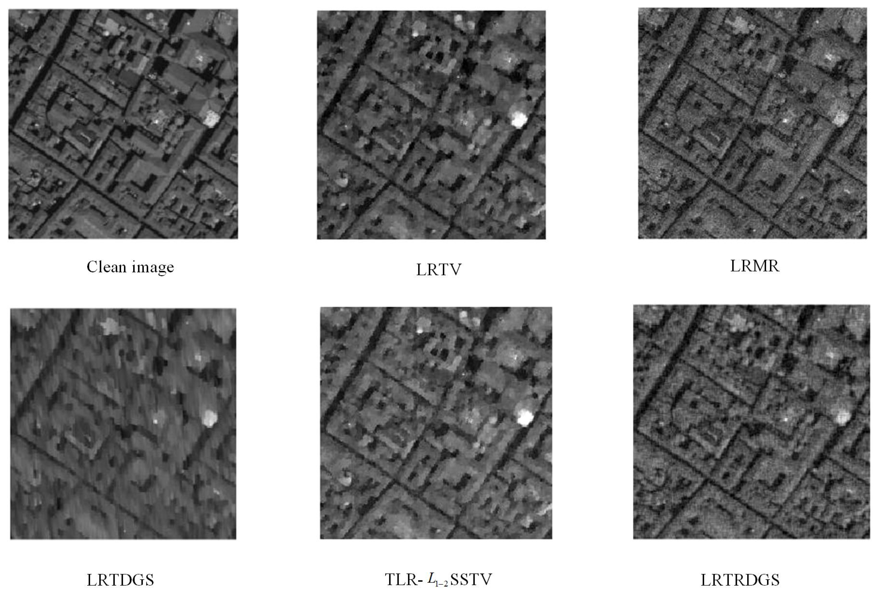
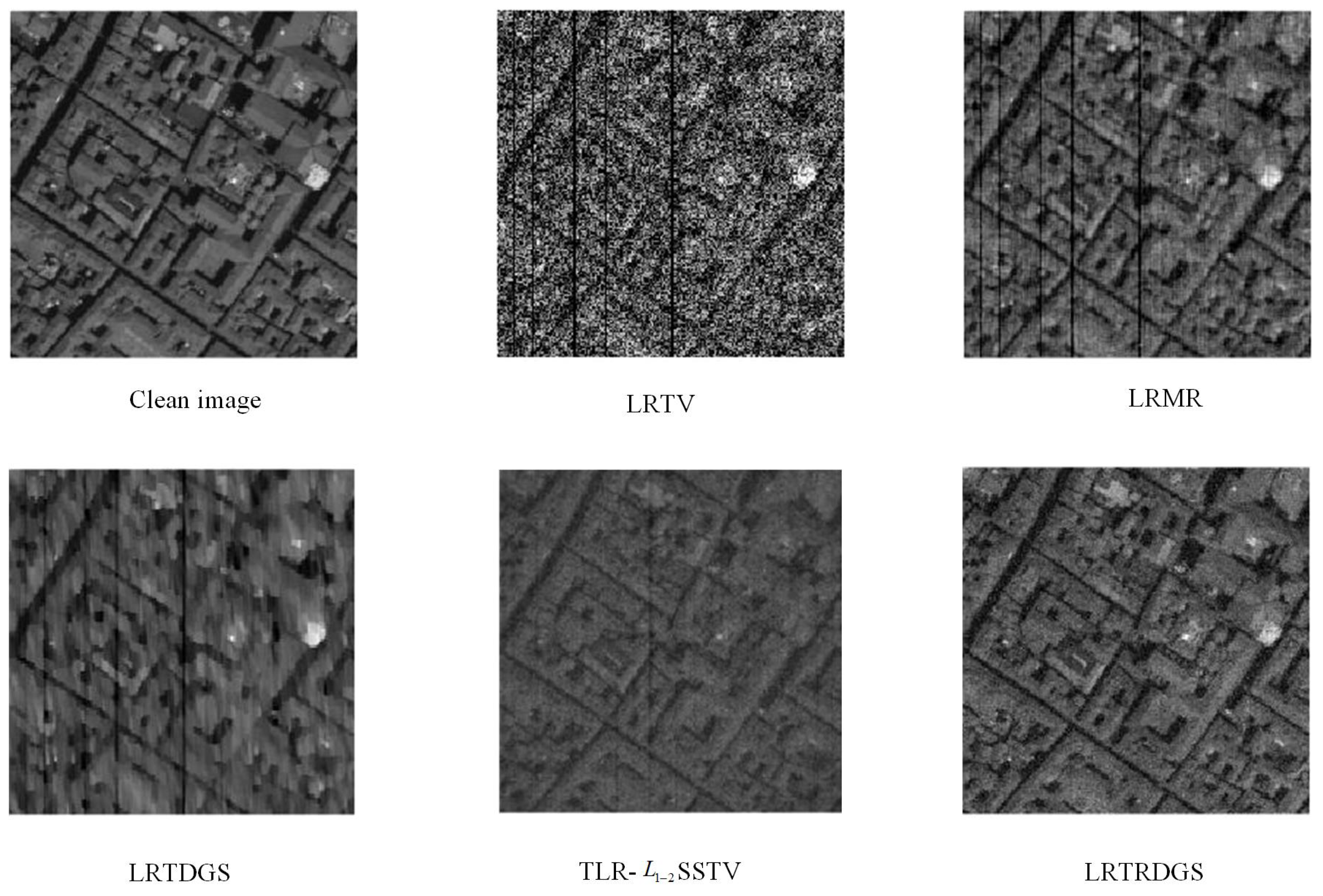
4. Experimental Results

In this section, we present the simulation outcomes for assessing the retrieval effectiveness of the novel LRTRDGS technique. The first dataset is the Washington DC Mall data, which is an image of Washington City, an aerial hyperspectral image acquired by the Hydice sensor, with a size of (256, 256, 160). Another dataset is the Pavia City Center dataset. This is an image of the city of Pavia in northern Italy captured by ROSIS sensors, taken by the Reflective Optical System Spectrometer, with dimensions (200, 200, 80) [28]. For comparison, we implement four typical HSI denoising methods, namely, total variation regularized low-rank matrix factorization (LRTV) [25], patchwise low-rank matrix approximation (LRMR) [29], weighted group sparsity-regularized low-rank tensor decomposition (LRTDGS) [16] and an $L_{1-2}$ spatial–spectral total variation regularized local low-rank tensor recovery model (TLR-$L_{1-2}$SSTV) [30]. The experiment applies the parameters proposed in the referenced article or the code authored by the investigator.

In this paper, three quantitative image quality indexes are used to evaluate the performance of the comparison methods, including the peak signal-to-noise ratio based on the characteristics of the human visual system (PSNR-HVS), mean structural similarity index measure (MSSIM) and erreur relative globale adimensionnelle desynthse (ERGAS). PSNR-HVS is a quality metric that measures the characteristics of the human visual system in a full-reference manner. MSSIM assesses the structural consistency to determine the similarity between the original hyperspectral image and the denoised hyperspectral image. Evaluating the fidelity of the denoised hyperspectral image, ERGAS incorporates the MSE of each band by assigning proper weights. To gauge the quality of the resultant denoised image, we employ three metrics:

$$\mathrm{PSNR}-\mathrm{HVS}=10log\left(\frac{{255}^2}{MS{E}_{HVS}}\right)$$

$$MS{E}_{HVS}=K\sum _{i=1}^{I-7}\sum _{j=1}^{J-7}\sum _{m=1}^8\sum _{n=1}^8{\left(\left(X{[m,n]}_{ij}-X{[m,n]}_{ij}^e\right)T_C[m,n]\right)}^2.$$

The PSNR-HVS can be adapted to different block sizes and is not computationally intensive. In this context, the height and width of the image are denoted as I and J, respectively, and an $8\times 8$ image block with the upper left corner at $(i,j)$ has $X_{ij}$ as its DCT coefficient. The DCT coefficient of the corresponding block in the original image is denoted as $X_{ij}^e$. The JPEG quantization table specified in the JPEG standard is represented as $T_c$, and K is calculated as $K=1/\left[\right(I-7\left)\right(J-7\left)64\right]$ [31].

$$\begin{array}{c}SSIM=\frac{\left(2{\mu }_x{\mu }_y+C_1\right)\left(2{\sigma }_{xy}+C_2\right)}{\left({\mu }_x^2+{\mu }_y^2+C_1\right)\left({\sigma }_x^2+{\sigma }_y^2+C_2\right)},\hfill \\ MSSIM(X,Y)=\frac{1}{Q}{\displaystyle \sum _{j=1}^Q}SSIM\left(x_j,y_j\right),\hfill \end{array}$$

where the constant $C_1$ represents ${\mu }_x^2+{\mu }_y^2$, while the $C_2$ value is equivalent to the $C_1$ value. The standard deviations of x and y are symbolized as ${\sigma }_x$ and ${\sigma }_y$ correspondingly. The initial image and the altered image are denoted as X and Y, respectively. The composition of the local window corresponding to the jth instance is indicated by $x_j$ and $y_j$, whereas the total number of local windows is denoted as $\mathrm{Q}$.

$$ERGAS=\sqrt{\frac{1}{P}\sum _{i=1}^P\frac{mes(re{f}_i,re{s}_i)}{Mea{n}_2\left(re{f}_i\right)}},$$

where $re{f}_i$ and $re{s}_i$ represent the reference image and recovered image of the ith band, respectively. P represents the number of bands.

In the experiment, all the reflectance values of the hyperspectral images are normalized to [0,1] for numerical calculation and visualization. To verify the performance of the method under different noise conditions, we add simulated noise to the simulated HSI data. The noise here mainly includes three types of noise: Gaussian noise, impulse noise and deadline noise. The deadline noise is caused by the uneven distribution of the sensor dark current and dark voltage, which will produce some dead lines in the image and affect the image quality. Here, we list five different noise situations:

Case 1 (i.i.d. Gaussian Noise): In this particular scenario, every band encounters independent Gaussian noise distributed uniformly with an average of zero.

Case 2 (i.i.d. Gaussian Noise + Deadline Noise): In this particular instance, following case 1, the band of 60–80 also experiences interference from a certain type of noise that disrupts the signal. For our analysis, we assign a random width to each stripe, ranging from 1 to 3, and a random number of stripes, ranging from 3 to 10.

Case 3 (i.i.d. Gaussian Noise + i.i.d. Impulse Noise): In this scenario, all bands encounter independent Gaussian noise that is distributed identically and exerts an average of zero. Additionally, they are subject to independent impulse noise that is identically distributed.

Case 4 (i.i.d. Gaussian Noise + i.i.d. Impulse Noise + Deadline Noise): In this specific scenario, as noted in case 3, the frequency bands ranging from 60 to 80 also experience interference from the dead line noise. To address this issue, we adopt a random approach for determining the width of each stripe, varying it between 1 and 3 units. Similarly, the number of stripes is selected randomly, ranging from 3 to 10.

Case 5 (non-i.i.d. Gaussian Noise + non-i.i.d. Impulse Noise + Deadline Noise): In this particular scenario, every single band experiences nonindependent identically distributed Gaussian noise that has an average of zero, as well as nonindependent identically distributed impulse noise. Additionally, the bands ranging from 60 to 80 encounter a certain level of dead line noise. The width of each stripe is determined in a random manner, falling between the range of 1 and 3. Furthermore, the number of stripes is randomly assigned between 3 and 10.

We provide the findings from our quantitative assessment of various comparison methods. The comparative outcomes of five HSI techniques on the Pavia City Center dataset are displayed in Table 1. Moreover, Table 2 demonstrates the comparative results of these five methods on the Washington DC Mall dataset. Notably, we have indicated the superior results, which are highlighted in bold within the tables. In this particular study, the Gaussian noise is denoted as $\theta$, while the impulse noise is represented as $\rho$. To visually demonstrate the comparative methods for HSI denoising, the denoising results at band 68 of the Pavia City Center dataset can be seen in Figure 3, Figure 4 and Figure 5. Additionally, the denoising result at band 61 of the Washington DC Mall dataset is shown in Figure 6, Figure 7 and Figure 8.

Table 1. Results of removing noise from the Pavia City Center dataset in different cases.

Case	Noise Level	Indicators	Noise	LRTV	LRMR	LRTDGS	TLR-${\mathit{L}}_{1-2}$SSTV	LRTRDGS
Case 1-1	$\theta =0.2$	PSNR-HVS	13.9932	28.7625	29.1682	26.9825	27.7324	29.8258
		MSSIM	0.1733	0.7904	0.8469	0.7195	0.8438	0.8471
		ERGAS	665.9520	168.4686	117.701	150.0049	148.9314	108.9523
		time (s)		117.272	99.203	72.022	88.274	100.32
Case 1-2	$\theta =0.4$	PSNR-HVS	7.9962	24.8261	24.3712	24.9912	24.6279	25.7813
		MSSIM	0.0510	0.6418	0.6469	0.6003	0.6834	0.6887
		ERGAS	1332.676	331.8135	206.591	188.9809	217.5825	178.4174
		time (s)		122.123	101.691	84.024	91.271	110.276
Case 2-1	$\theta =0.2$ +Deadline	PSNR-HVS	10.7621	26.1072	26.4181	25.5719	27.4619	27.5891
		MSSIM	0.0871	0.6982	0.7445	0.6435	0.8401	0.8416
		ERGAS	999.3376	233.1479	163.708	182.5346	155.4789	152.6477
		time (s)		119.718	100.178	81.651	87.874	103.782
Case 2-2	$\theta =0.4$ +Deadline	PSNR-HVS	7.9963	23.9574	24.3571	24.7893	23.9965	24.9979
		MSSIM	0.0505	0.6202	0.6477	0.5918	0.6736	0.6762
		ERGAS	1330.449	348.6010	208.053	201.1706	230.4959	190.4651
		time (s)		124.267	104.781	86.983	91.784	113.926
Case 3-1	$\theta =0.3$ +$\rho =0.1$	PSNR-HVS	9.1271	25.2875	24.3688	25.2870	25.2769	25.9945
		MSSIM	0.0640	0.6658	0.6700	0.6207	0.7212	0.7223
		ERGAS	1169.856	276.2930	202.819	184.5704	200.0335	166.8273
		time (s)		98.962	119.267	74.232	85.127	103.261
Case 3-2	$\theta =0.4$ +$\rho =0.15$	PSNR-HVS	6.9612	22.9659	22.4892	23.7926	23.8920	23.9864
		MSSIM	0.0362	0.5578	0.5565	0.5448	0.6130	0.6188
		ERGAS	1526.545	351.0957	257.677	216.6734	247.5929	215.5840
		time (s)		97.122	116.968	78.197	85.969	101.206
Case 4-1	$\theta =0.4$ +$\rho =0.15$ +Deadline	PSNR-HVS	7.2871	23.3789	23.9865	24.8547	23.6794	24.2688
		MSSIM	0.0404	0.5800	0.5887	0.5598	0.6042	0.6277
		ERGAS	1462.063	359.3642	232.914	211.6882	253.7716	208.3434
		time (s)		100.271	120.861	81.994	89.275	111.788
Case 4-2	$\theta =0.3$ +$\rho =0.075$ +Deadline	PSNR-HVS	10.1122	25.9769	25.0153	25.1878	24.9962	25.9014
		MSSIM	0.0685	0.6798	0.6880	0.6200	0.7242	0.7350
		ERGAS	1128.251	269.8426	189.770	191.0023	205.3501	174.1756
		time (s)		99.882	117.962	80.997	87.291	108.782
Case 5-1	$\theta =U(0.1,0.2)$ +$\rho =U(0.2,0.3)$ +Deadline	PSNR-HVS	11.5786	26.8971	26.2788	26.0165	26.8961	26.9987
		MSSIM	0.1003	0.7242	0.7498	0.6700	0.8258	0.8666
		ERGAS	942.5571	264.2848	162.700	170.5190	165.8885	154.6694
		time (s)		100.978	118.653	82.878	87.998	109.004
Case 5-2	$\theta =U(0.4,0.5)$ +$\rho =U(0.01,0.1)$ +Deadline	PSNR-HVS	6.8768	23.6871	23.0902	24.8910	23.8760	24.6891
		MSSIM	0.0373	0.5704	0.5776	0.5545	0.6139	0.6391
		ERGAS	1551.881	381.8465	236.612	212.0504	250.6892	199.8251
		time (s)		100.101	118.433	84.903	88.022	110.057

The best results are highlighted by bold.

Table 2. Results of removing noise from the Washington DC Mall dataset in different cases.

Case	Noise Level	Indicators	Noise	LRTV	LRMR	LRTDGS	TLR-${\mathit{L}}_{1-2}$SSTV	LRTRDGS
Case 1-1	$\theta =0.2$	PSNR-HVS	14.0163	27.901	29.7813	28.082	27.9870	30.8762
		MSSIM	0.2560	0.8160	0.9046	0.8233	0.8928	0.9120
		ERGAS	751.882	162.6289	120.4509	145.6978	151.9219	105.1567
		time (s)		65.903	125.355	101.05	168.771	129.875
Case 1-2	$\theta =0.4$	PSNR-HVS	8.0724	24.8962	24.9809	25.8565	21.6804	26.8577
		MSSIM	0.0885	0.6706	0.7563	0.7345	0.4456	0.8046
		ERGAS	1503.76	265.8668	211.9395	188.3212	314.1924	168.3608
		time (s)		68.384	129.074	116.272	171.283	134.115
Case 2-1	$\theta =0.2$ +Deadline	PSNR-HVS	14.0758	27.9572	29.6927	28.0184	26.9483	30.0078
		MSSIM	0.2543	0.8121	0.9031	0.8234	0.8689	0.8996
		ERGAS	753.640	159.1033	122.6426	146.1582	167.6949	120.0915
		time (s)		66.282	118.784	110.709	165.203	130.673
Case 2-2	$\theta =0.4$ +Deadline	PSNR-HVS	8.0034	24.9894	24.8892	25.8762	24.0708	26.9950
		MSSIM	0.0880	0.6662	0.7556	0.7393	0.7898	0.7987
		ERGAS	1503.85	258.5927	213.5223	190.8474	212.9540	181.1324
		time (s)		63.228	112.783	106.889	159.995	127.257
Case 3-1	$\theta =0.2$ +$\rho =0.1$	PSNR-HVS	11.9947	27.7842	25.0749	27.9302	27.8404	30.7730
		MSSIM	0.1701	0.7808	0.7993	0.8056	0.8755	0.9012
		ERGAS	1047.90	175.0467	213.6028	153.4816	161.8219	112.6899
		time (s)		65.893	116.291	109.680	160.003	127.982
Case 3-2	$\theta =0.3$ +$\rho =0.2$	PSNR-HVS	7.9956	24.0949	21.0092	24.8709	24.0825	26.9904
		MSSIM	0.0827	0.6465	0.6547	0.7162	0.7646	0.8026
		ERGAS	1529.86	258.4262	340.4201	204.1038	230.8225	80.2526
		time (s)		66.113	116.982	111.293	160.904	128.040
Case 4-1	$\theta =0.4$ +$\rho =0.1$ +Deadline	PSNR-HVS	7.2837	23.8392	23.0392	25.1039	23.9029	25.9372
		MSSIM	0.0716	0.6058	0.6908	0.7066	0.7450	0.7553
		ERGAS	1672.07	303.2406	264.5094	207.8214	236.6696	201.1609
		time (s)		70.284	119.103	117.739	165.492	130.265
Case 4-2	$\theta =0.2$ +$\rho =0.3$ +Deadline	PSNR-HVS	8.9829	25.0284	18.9271	26.0174	25.0172	26.8740
		MSSIM	0.0849	0.6982	0.6003	0.7508	0.8120	0.8245
		ERGAS	1472.33	241.7256	449.2673	185.5257	204.7093	174.2441
		time (s)		69.027	118.685	115.336	162.870	128.278
Case 5-1	$\theta =U(0.3,0.4)$ +$\rho =U(0.1,0.2)$ +Deadline	PSNR-HVS	7.7944	23.8902	21.9080	24.9823	23.9802	25.6890
		MSSIM	0.0780	0.6163	0.6715	0.7083	0.7525	0.7677
		ERGAS	1584.39	307.9037	301.3547	208.4486	236.4430	198.0863
		time (s)		73.282	125.394	117.003	166.682	131.082
Case 5-2	$\theta =U(0.2,0.3)$ +$\rho =U(0.2,0.3)$ +Deadline	PSNR-HVS	8.5902	24.6823	19.9322	25.8948	24.7839	26.7735
		MSSIM	0.0860	0.6667	0.6278	0.7293	0.7847	0.8052
		ERGAS	1494.11	271.4693	392.7230	198.8723	222.9171	184.1283
		time (s)		71.942	123.463	110.228	160.382	129.735

The best results are highlighted by bold.

Figure 3. Denoising results of case 3-1 on the Pavia City Center dataset.

Figure 4. Denoising results of case 4-2 on the Pavia City Center dataset.

Figure 5. Denoising results of case 5-1 on the Pavia City Center dataset.

Figure 6. Denoising results of case 1-2 on the Washington DC Mall dataset.

Figure 7. Denoising results of case 4-1 on the Washington DC Mall dataset.

Figure 8. Denoising results of case 5-2 on the Washington DC Mall dataset.

In addition, Figure 3 and Figure 6 show the denoising results of the testing HSIs for case 1 and case 3, respectively. LRTRDGS, the method that is being proposed, demonstrates exceptional outcomes in terms of visual quality in comparison to the alternative methods. LRTRDGS showcases its ability to eliminate both Gaussian noise and impulse noise while simultaneously maintaining the fundamental structure of HSI. LRMR and TLR-$L_{1-2}$SSTV produce results with some noise. LRTV and LRTDGS can eliminate hyperspectral image noise, but some details may be lost in the process. For cases 2, 4 and 5, the focus is on evaluating the performance of deadline noise removal. Figure 4 and Figure 5 depict the denoising outcomes obtained from the Pavia City Center dataset. Similarly, the denoising results for the Washington DC Mall dataset are shown in Figure 7 and Figure 8. The proposed LRTRDGS method demonstrates its capability to effectively remove unexpected deadline noise while preserving the underlying HSI details. The results of LRTV and LRTDGS also show a small amount of deadline noise. Additionally, we present the values of PSNR-HVS and MSSIM for each frequency band in the Washington DC Mall simulation dataset case 3-1 (Figure 9 and Figure 10) and case 5-1 (Figure 11 and Figure 12). The results demonstrate that our proposed LRTRDGS method outperforms the other methods in terms of both PSNR-HVS and MSSIM. Specifically, when applied to two different hyperspectral images, the LRTRDGS method achieves superior results compared to the four other comparison methods. These findings suggest that tensor ring decomposition plays a positive role in denoising hyperspectral images.

Figure 9. PSNR-HVS of the different methods for each band of case 3-1 on the Washington DC Mall dataset.

Figure 10. MSSIM of the different methods for each band of case 3-1 on the Washington DC Mall dataset.

Figure 11. PSNR-HVS of the different methods for each band of case 5-1 on the Washington DC Mall dataset.

Figure 12. MSSIM of the different methods for each band of case 5-1 on the Washington DC Mall dataset.

Our proposed LRTRDGS does not have an advantage in CPU time. This is because the tensor ring structure is slightly more complex, resulting in longer calculation times. Because of the use of tensor rings, our proposed method achieves better results in quantification (Table 1 and Table 2) and visualization (Figure 6, Figure 7, Figure 8, Figure 9, Figure 10, Figure 11 and Figure 12).

In the LRTRDGS method, the selection of parameters determines the denoising results of the hyperspectral images. The parameters include the total variation regularization parameter $\delta$, sparse noise regularization parameter ${\lambda }_1$, Gaussian noise regularization parameter ${\lambda }_2$, the rank of the tensor ring $r=[r_1.r_2,r_3]$, adjacent operator parameter $\sigma$ and other parameters $v_1,v_2,v_3,v_4,v_5$ and $v_6$. Based on the simulation data of case 3 in the Washington DC Mall dataset, the influence of the parameters is discussed.

The influence of the total variation regularization parameter $\delta$ is shown below. Figure 13 shows the PSNR value for $\delta$ values of 0.01, 0.05, 0.1, 0.5, 1 and 1.5. The results show that $\delta =0.05$ has the best effect.

Figure 13. Influence of parameter $\delta$.

Below is the demonstration of the impact of the regularization parameter ${\lambda }_1$ on the sparse noise limitation, which restricts the extent of the sparsity in sparse noise. We set ${\lambda }_1=\frac{A\times {10}^6}{\sqrt{M\times N}}$, where M is the height of the hyperspectral band and N is the width of the hyperspectral band. Figure 14 shows the PSNR values when A is set to 1, 2, 5, 8, 10, 15, 20, 25, 30, 40 and 50. The results show that $A=130$ achieves the best PSNR value.

Figure 14. Influence of parameter A.

Here, we consider the influence of the sparse noise regularization parameter ${\lambda }_2$. This parameter plays a role in limiting the sparsity of Gaussian noise. Figure 15 shows the PSNR values when ${\lambda }_2$ is set to 100, 200, 210, 220, 230, 240, 250, 260, 270, 280, 290 and 300. The results show that ${\lambda }_2=210$ yields the best PSNR value.

Figure 15. Influence of parameter ${\lambda }_2$.

The influence of the rank of the tensor ring $r=[r_1,r_2,r_3]$, which is an important parameter to control the correlation of tensors, is discussed. In order to streamline the determination of the tensor ring’s rank, we make the assumption that the ranks of the second and third dimensions are identical, denoted as $r_2=r_3$. The PSNR values vary under different tensor ring ranks, as shown in Figure 16. In order to achieve a balance between the robustness of the tensor ring rank and the effectiveness of the denoising results, we set the tensor ring rank differently in different noise environments. For the previously discussed case, we set the tensor ring to $r=[7,14,14]$.

Figure 16. Influence of parameter r.

We consider the influence of the adjacent operator parameter $\sigma$, which is used to limit the step size of a neighboring operator. Here, we select the sets 0.0001, 0.0005, 0.001, 0.005, 0.01 and 0.05 as the test data. Figure 17 shows the data test results. Finally, $\sigma =0.01$ is selected as the optimal value.

Figure 17. Influence of parameter $\sigma$.

Regarding the influence of parameter $\mu$, Figure 18 shows the recovery results for changes in the sets 0.001, 0.005, 0.006, 0.007, 0.01, 0.05 and 0.1. The results show that $\mu =0.006$ has the best effect.

Figure 18. Influence of parameter $\mu$.

Regarding the influence of the parameters $v_1,v_2,v_3,v_4,v_5$ and $v_6$, Figure 19, Figure 20, Figure 21, Figure 22, Figure 23 and Figure 24 show the data analyzed. Finally, we chose $v_1=1,v_2=0.8,v_3=0.9,v_4=1.1,v_5=1$ and $v_6=1$ as the best results.

Figure 19. Influence of parameter $v_1$.

Figure 20. Influence of parameter $v_2$.

Figure 21. Influence of parameter $v_3$.

Figure 22. Influence of parameters $v_4$.

Figure 23. Influence of parameter $v_5$.

Figure 24. Influence of parameter $v_6$.

Because the parameters $\mathcal{P}$, $\mathcal{S}$, $\mathcal{N}$ and others are solved using simple algebraic calculations, our main focus is on the time spent on $\mathcal{X}$ and $\mathcal{Q}$. $h\times w\times b$ is the size of the hyperspectral image affected by noise. A tensor ring representation is used to estimate $\mathcal{G}$ for updating $\mathcal{X}$. Assuming that the size is $\mathcal{X}\in {\mathbb{R}}^{I\times I\times I}$ and the TR rank is set as $r_1=r_2=r_3=r$, there is a cost of O($r^6$ + $I^2{r}^4$ + $I^3{r}^2$) to $\mathcal{X}$ in each iteration. $O\left(D_{1}log{D}_1\right)$ refers to the computational complexity of the FFT, where $D_1$ is the size of the data. Consequently, the cost of updating the subproblem of $\mathcal{Q}$ is denoted as $O\left(hwblog\right(hwb\left)\right)$. According to the above, the proposed algorithm has a complexity of O($r^6$ + $I^2{r}^4$ + $I^3{r}^2$ + h w b log(h w b)).

At last, numerical experiments are conducted to verify the convergence of the proposed algorithm. Figure 25 shows the variation in R with the number of iterations of LRTRDGS for hyperspectral reconstructions, where $R=\frac{\parallel {\mathcal{X}}^p-{\mathcal{X}}^{p+1}{\parallel }_F^2}{{\parallel \mathcal{Y}\parallel }_F^2}$. As the number of iterations increases, R approaches zero.

Figure 25. Change in the value R for the hyperspectral reconstructed images versus the number of iterations.

5. Conclusions

A weighted group sparse regularization tensor ring decomposition method for hyperspectral image restoration is proposed. The global spatial–spectral correlation model of hyperspectral images is tensor ring decomposition. Using weighted group sparsity to constrain the spectral dimension of spatial difference images is more reasonable than using total variation regularization. The effectiveness of hyperspectral image restoration is demonstrated by the experimental findings of the LRTRDGS method proposed. The implementation of LRTRDGS provides a means to effectively mitigate noise while preserving the intricate textural features of HSI. For further exploration of the spatial domain of HSI, it is recommended to consider representation-based subspace low-rank learning methods that provide more accurate regularization of nonlocal self-similarity. Additionally, it is worth investigating image compression techniques with a low-rank degree.

References

- Stuart, M.B.; McGonigle, A.J.S.; Willmott, J.R. Hyperspectral Imaging in Environmental Monitoring: A Review of Recent Developments and Technological Advances in Compact Field Deployable Systems. Sensors 2019, 19, 3071. [Google Scholar] [CrossRef]
- Hanuš, J.; Slezák, L.; Fabiánek, T.; Fajmon, L.; Hanousek, T.; Janoutová, R.; Kopkáně, D.; Novotný, J.; Pavelka, K.; Pikl, M.; et al. Flying Laboratory of Imaging Systems: Fusion of Airborne Hyperspectral and Laser Scanning for Ecosystem Research. Remote Sens. 2023, 15, 3130. [Google Scholar] [CrossRef]
- Schodlok, M.C.; Frei1, M.; Segl, K. Implications of new hyperspectral satellites for raw materials exploration. Miner. Econ. 2022, 35, 495–502. [Google Scholar] [CrossRef]
- Avola, G.; Matese, A.; Riggi, E. Precision Agriculture Using Hyperspectral Images. Remote Sens. 2023, 15, 1917. [Google Scholar] [CrossRef]
- Moncholi-Estornell, A.; Cendrero-Mateo, M.P.; Antala, M.; Cogliati, S.; Moreno, J.; Van Wittenberghe, S. Enhancing Solar-Induced Fluorescence Interpretation: Quantifying Fractional Sunlit Vegetation Cover Using Linear Spectral Unmixing. Remote Sens. 2023, 15, 4274. [Google Scholar] [CrossRef]
- Naß, A.; van Gasselt, S. A Cartographic Perspective on the Planetary Geologic Mapping Investigation of Ceres. Remote Sens. 2023, 15, 4209. [Google Scholar] [CrossRef]
- Sharma, S.R.; Singh, B.; Kaur, M. A hybrid encryption model for the hyperspectral images: Application to hyperspectral medical images. Multimed. Tools Appl. 2023. [Google Scholar] [CrossRef]
- Bedini, E. The use of hyperspectral remote sensing for mineral exploration: A review. J. Hyperspectral Remote Sens. 2017, 7, 189–211. [Google Scholar] [CrossRef]
- Haagsma, M.; Hagerty, C.H.; Kroese, D.R.; Selker, J.S. Detection of soil-borne wheat mosaic virus using hyperspectral imaging: From lab to field scans and from hyperspectral to multispectral data. Precis. Agric. 2023, 24, 1030–1048. [Google Scholar] [CrossRef]
- Adjovu, G.E.; Stephen, H.; James, D.; Ahmad, S. Measurement of Total Dissolved Solids and Total Suspended Solids in Water Systems: A Review of the Issues, Conventional, and Remote Sensing Techniques. Remote Sens. 2023, 15, 3534. [Google Scholar] [CrossRef]
- Renard, N.; Bourennane, S.; Blanc-Talon, J. Denoising and dimensionality reduction using multilinear tools for hyperspectral images. IEEE Trans. Geosci. Remote Sens. 2008, 5, 138–142. [Google Scholar] [CrossRef]
- Chen, Y.; Huang, T.Z.; Zhao, X.L. Destriping of multispectral remote sensing image using low-rank tensor decomposition. IEEE J. Sel. Top. Appl. Earth Obs. Remote Sens. 2018, 11, 4950–4967. [Google Scholar] [CrossRef]
- Liu, X.; Bourennane, S.; Fossati, C. Denoising of hyperspectral images using the PARAFAC model and statistical performance analysis. IEEE Trans. Geosci. Remote Sens. 2012, 50, 3717–3724. [Google Scholar] [CrossRef]
- Guo, X.; Huang, X.; Zhang, L.; Zhang, L. Hyperspectral image noise reduction based on rank-1 tensor decomposition. ISPRS J. Photogramm. Remote Sens. 2013, 83, 50–63. [Google Scholar] [CrossRef]
- Fan, H.; Li, C.; Guo, Y.; Kuang, G.; Ma, J. Spatial Cspectral total variation regularized low-rank tensor decomposition for hyperspectral image denoising. IEEE Trans. Geosci. Remote Sens. 2018, 56, 6196–6213. [Google Scholar] [CrossRef]
- Chen, Y.; He, W.; Yokoya, N.; Huang, T.Z. Hyperspectral Image Restoration Using Weighted Group Sparsity-Regularized Low-Rank Tensor Decomposition. IEEE Trans. Cybern. 2020, 50, 3556–3570. [Google Scholar] [CrossRef]
- Wang, Y.; Peng, J.; Zhao, Q.; Meng, D.; Leung, Y.; Zhao, X.-L. Hyperspectral image restoration via total variation regularized low-rank tensor decomposition. IEEE J. Sel. Top. Appl. Earth Obs. Remote Sens. 2018, 11, 1227–1243. [Google Scholar] [CrossRef]
- Xue, J.; Zhao, Y.; Liao, W.; Chan, J.C. Nonlocal low-rank regularized tensor decomposition for hyperspectral image denoising. IEEE Trans. Geosci. Remote Sens. 2019, 57, 5174–5189. [Google Scholar] [CrossRef]
- Xie, Y.; Qu, Y.; Tao, D.; Wu, W.; Yuan, Q.; Zhang, W. Hyperspectral Image Restoration via Iteratively Regularized Weighted Schatten p-Norm Minimization. IEEE Trans. Geosci. Remote Sens. 2016, 54, 4642–4659. [Google Scholar] [CrossRef]
- Zhao, Q.; Zhou, G.; Xie, S.; Zhang, L.; Cichocki, A. Tensor Ring Decomposition. arXiv 2016, arXiv:1606.05535. [Google Scholar] [CrossRef]
- Zhao, Q.; Sugiyama, M.; Yuan, L.; Cichocki, A. Learning Efficient Tensor Representations with Ring-structured Networks. In Proceedings of the ICASSP 2019—2019 IEEE International Conference on Acoustics, Speech and Signal Processing (ICASSP), Brighton, UK, 12–17 May 2019. [Google Scholar]
- Wang, W.; Aggarwal, V.; Aeron, S. Efficient low rank tensor ring completion. In Proceedings of the IEEE International Conference on Computer Vision, Venice, Italy, 22–29 October 2017. [Google Scholar]
- He, W.; Yokoya, N.; Yuan, L.; Zhao, Q. Remote Sensing Image Reconstruction Using Tensor Ring Completion and Total Variation. IEEE Trans. Geoence Remote Sens. 2019, 57, 8998–9009. [Google Scholar] [CrossRef]
- Rudin, L.I.; Osher, S.; Fatemi, E. Nonlinear total variation based noise removal algorithms. Phys. D Nonlinear Phenom. 1992, 60, 259–268. [Google Scholar] [CrossRef]
- He, W.; Zhang, H.; Zhang, L.; Shen, H. Total-variation-regularized low-rank matrix factorization for hyperspectral image restoration. IEEE Trans. Geosci. Remote Sens. 2016, 54, 178–188. [Google Scholar] [CrossRef]
- Wei, H.; Zhang, H.; Shen, H.; Zhang, L. Hyperspectral Image Denoising Using Local Low-Rank Matrix Recovery and Global Spatial-CSpectral Total Variation. IEEE J. Sel. Top. Appl. Earth Obs. Remote Sens. 2018, 11, 1–17. [Google Scholar]
- Kolda, T.G.; Bader, B.W. Tensor decompositions and applications. SIAM Rev. 2009, 51, 455–500. [Google Scholar] [CrossRef]
- Hyperspectral Images. Available online: https://engineering.purdue.edu/~biehl/MultiSpec/hyperspectral.html (accessed on 3 July 2023).
- Zhang, H.; He, W.; Zhang, L.; Shen, H.; Yuan, Q. Hyperspectral image restoration using low-rank matrix recovery. IEEE Trans. Geosci. Remote Sens. 2014, 52, 4729–4743. [Google Scholar] [CrossRef]
- Zeng, H.; Xie, X.; Cui, H.; Yin, H.; Ning, J. Hyperspectral Image Restoration via Global L1-2 Spatial-Spectral Total Variation Regularized Local Low-Rank Tensor Recovery. IEEE Trans. Geosci. Remote Sens. 2021, 59, 3309–3325. [Google Scholar] [CrossRef]
- Valizadeh, S.; Nasiopoulos, P.; Ward, R. Perceptual rate distortion optimization of 3D–HEVC using PSNR-HVS. Multimed. Tools Appl. 2018, 77, 22985–23008. [Google Scholar] [CrossRef]