Resilience Analysis of Traffic Network under Emergencies: A Case Study of Bus Transit Network

Abstract

With the continuous development of public transportation, the impact of unexpected events on the operation of bus networks has become increasingly severe due to the growing demand for public transportation and passenger volume. To accurately assess the impact of unexpected events on the operation of bus networks and scientifically evaluate their resilience, this paper proposes a framework for analyzing the resilience of bus networks. With the aim of providing scientific evidence to enhance the reliability of public transportation networks, this framework can be used to determine the resilience of bus networks to unexpected events. The main contributions of this framework include three aspects: 1. Construction of the CRITIC–entropy weighting model for screening and calculating key indicators of the resilience of the bus network; 2. Use of resilience cycle theory to construct a model for analyzing the resilience of bus routes, and design a set of resilience quantification factors to calculate the resilience of bus routes; 3. Use of complex network theory to construct a model for analyzing the resilience of the bus network, by taking the bus route resilience obtained in the second step as the edge weight to calculate the resilience of the bus network. This paper takes the Beijing public transit system as an example and uses real data to verify the accuracy, scientificity, and feasibility of the proposed framework for analyzing the resilience of public transit networks to sudden events. The resilience analysis framework constructed in this paper has improved the existing research on transportation network resilience in theoretical aspects. Furthermore, the results outputted by this framework can provide a decision-making basis for network adjustment and disaster recovery for the management departments of public transportation networks in practical applications.

1. Introduction

1.1. Research Background

In recent years, public transportation has become the main mode of daily travel for the general public due to its high capacity, low cost, and reliable on-time performance. China’s 12th Five-Year Plan has made significant achievements in urban transportation construction, with the total amount of urban public transportation constantly increasing and the passenger volume gradually increasing. The “public transportation priority” policy was mentioned in China’s 12th Five-Year Plan for National Economic and Social Development, which calls for the implementation of a “public transportation priority” development strategy and the vigorous development of urban public transportation systems. It can be said that urban public transportation in China is in a period of great development and construction. Urban public transportation here generally refers to conventional public transportation such as buses and rail transit within the city. Among them, conventional buses refer to public transportation routes developed by local public transportation companies after applying to relevant national departments and are a public interest transportation mode that receives policy subsidies. The bus network studied in this article refers to the transportation network composed of daily operating routes of conventional buses in the city.

In recent years, there have been frequent sudden incidents in public transportation in China, such as the collapse of Shanghai Metro Line 12 in 2012, the flooding of bus and subway stations in Wuhan due to heavy rain in 2016, and the backflow flooding in Zhengzhou’s metro caused by heavy rain in 2021. In central cities in China, the harm caused by sudden incidents to urban public transportation is particularly evident. For example, during the heavy rain on 21 July 2012, in Beijing, the disaster affected an area of 16,000 square kilometers and 1.9 million people, causing various degrees of damage to many transportation infrastructures, including bridges, roads, and networks. In total, there were 63 major flooded roads and 31 road collapses. Twelve stations on five subway lines were closed due to flooding, causing economic losses of up to billions of RMB, according to statistics. In 2013, a major rainstorm hit Shanghai on September 13th, causing severe flooding on more than 80 roads in the city. Due to the heavy rain occurring during rush hour, many transportation routes were paralyzed, seriously affecting citizens’ normal commuting and travel. The occurrence of public transportation emergencies can cause damage to public facilities and traffic congestion on accident-prone routes, affecting citizens’ normal travel. In more serious cases, it may result in casualties, paralysis of the transportation network, and lead to a severe public relations crisis.

Due to the increasingly dense urban space and population distribution, as well as the increasingly diverse structure of urban transportation networks, the uncertainties and unknown risks faced by the development of public transportation networks are unprecedentedly complex. The potential impacts and catastrophic consequences are becoming more significant. However, when facing these disturbances and disruptions, the reactions of different public transportation networks vary greatly. Some networks become paralyzed after experiencing emergencies, unable to quickly digest and eliminate the negative impacts of the emergencies, while others can quickly overcome the adverse impacts of emergencies, and even take this opportunity to improve their own mechanisms for dealing with emergencies. The essential reason for the different results is the difference in resilience of the public transportation networks: a network with strong resilience has a strong ability to adapt and recover from disturbances caused by emergencies, while a network with weak resilience has a relatively lagging reaction capability, insufficient adaptability, and a longer recovery period.

Based on the above background, in order to further explore the performance changes in the bus network under emergency situations, modeling and analyzing the resilience of the bus network has become the key to bus operations. However, in the process of modeling and analyzing the actual resilience of the bus network, how should the indicators that best represent the operating performance of the bus network be selected? How should the spatiotemporal dynamics and structural statics of the bus network be combined to analyze its resilience? These are urgent issues that need to be addressed in the current research on bus network resilience. In the context of practical problems, establishing a framework for studying the resilience of the bus network undoubtedly has significant academic and social value.

1.2. Motivation and Contribution

The main significance of this research lies in the qualitative and quantitative analysis of the resilience of public transit networks from the perspective of their spatiotemporal dynamics and structural statics, which solves the problem faced by transit network managers who hold a large amount of operational monitoring data but cannot comprehensively and systematically grasp the state and changes in transit networks under the influence of unexpected events. With the proposed framework and model for analyzing the resilience of transit networks in this article, the ability of transit networks to resist the impact of unexpected events can be accurately evaluated. This research provides transit network managers with intuitive and trustworthy evaluation conclusions, while also laying a solid theoretical and data foundation for optimizing transit networks and improving the study of network resilience.

This paper aims to analyze the resilience of urban bus networks in the face of unexpected events. In response to the lack of research frameworks and experimental demonstrations in the current academic research on bus network resilience analysis, this paper comprehensively applies indicator evaluation methods, resilience cycle theory, and complex network theory to construct a modeling and analysis framework for the resilience of bus networks. This paper has significant innovative significance in the field of bus network resilience research, with three main innovations:

(1)

In response to the problem of how to scientifically select operational indicators that reflect the resilience of urban bus networks, this paper designed an indicator evaluation model based on the CRITIC–entropy weight method using actual bus network data. By combining multiple indicator dimensions through the idea of a composite evaluation model, the scientificity of indicator selection is improved.

(2)

In response to the temporal and spatial dynamics of urban bus networks, this paper constructed a line resilience analysis model based on the resilience cycle theory and a set of resilience quantification factors. The example analysis results show that the bus line resilience analysis model based on the resilience cycle theory can accurately reflect the degree of impact of sudden events on bus lines from the perspective of temporal and spatial dynamics, with lines having higher resilience values being less affected.

(3)

In response to the structural static nature of urban bus networks, this paper abstracted the bus network into an undirected weighted complex network and based on the centrality concept of complex network theory, constructed a bus network resilience analysis model. The example analysis results show that this model accurately reflects the resilience value of the entire bus network from the perspective of the network’s structural static nature.

The research framework and models proposed in this paper for the analysis of the resilience of urban bus networks not only fill the theoretical research gap in the field of public transportation network resilience but also provide qualitative and quantitative analysis tools and methods for the operation and management departments of bus networks regarding their resilience.

1.3. Paper Organization

The organizational structure of this article is as follows: Section 1 is the introduction, which introduces the research background, significance, and main academic contributions of this article. Section 2 introduces the current research on resilience and the state of resilience research in the transportation field. Section 3 introduces the resilience analysis framework and model for the public transit network proposed in this article and validates the proposed model. Section 4 introduces the real data used in this article, and then conducts case studies on the proposed framework using real data. Section 5 summarizes and prospects the research in this article.

2. Related Literature

2.1. Resilience Theory Research

The term “resilience” originates from the Latin word “resilire”, which means “to rebound or recoil”. In 1807, the physicist Thomas Young first used the term to describe elastic deformation in the context of materials science [1]. In 1973, Holling first introduced resilience as a concept in the field of sustainability science [2]. He defined resilience as “the persistence of relationships within a system and is a measure of the ability of these systems to absorb changes in state variables, driving variables, and parameters” [3]. In subsequent multidisciplinary research, the concept of resilience has been widely applied, including in the fields of ecology [4], economics, transportation [5], supply chain management [6], strategic management [7], and safety engineering [8], among others. The number of resilience studies from 1973 to the present is shown in Figure 1 [9].

Figure 1. Number of resilience studies during 1973–2022.

However, despite the widespread application of resilience research, the concept remains unclear in many interdisciplinary developments and studies [10]. Based on this, Anderies et al. argue that the concept of resilience may inherently have fuzzy attributes, as it has different definitions when serving specific goals in different disciplines. Resilience is more of a way of thinking for analyzing problems rather than a fixed concept [11]. Therefore, if there is no consensus on the ambiguity of the concept of resilience in various fields of research, a rigid definition of the concept of resilience may cause confusion. Carpenter et al. suggest that systematic thinking is necessary for resilience research and that each resilience scenario needs to be defined, starting with clarifying the system definition, system boundaries, external environment, and interactions between the system and the external environment, and then identifying changes in system inputs and outputs [12].

The current academic research on resilience lacks systematic empirical studies [10]. Resilience research is mainly conceptual and focuses on developing a static knowledge base for related research fields by establishing basic concepts and principles [10]. The related research in various fields based on resilience has mainly gone through the following three stages:

(1)

Fragility.

The term “fragility” has many meanings, but it is usually associated with the vulnerability of a system to external influences. Miller et al. conducted a systematic study of fragility in the context of climate change and proposed four hypotheses for assessing fragility in the process of adapting to climate change. Finally, they defined fragility as the degree to which a system is affected by climate change [13]. Eriksen and colleagues defined the concept of fragility from a more macro perspective as the response of a system to a series of influences, including the degree of exposure to external stresses and sensitivity to perturbations [14]. The concept of fragility is inherently complex, involving multiple variables, and can be considered a dynamic entity [15]. In more specific studies of fragility, Joakim identified the conceptual linkage between fragility, resilience, and adaptability [16]. Based on this representation, Pamungkas’s study considered resilience as a subset or component of a system’s response capacity, which involves the ability of a system to adjust and regulate its response to disturbances, use any available measures, and respond to the consequences of system changes [17]. It is therefore generally believed among researchers that studies on system fragility are often conducted as an aspect of resilience research [18].

(2)

Adaptability.

As Petersen et al. showed in their example of studying the resilience of social–ecological systems, system adaptability is related to the creation of novelty and self-learning mechanisms in ecological systems [19]. Whitney describes system adaptability as ecological resilience acting as the system’s robustness to changes in resilience [20]. Chen et al. proposed a conceptual framework for assessing the adaptability of urban water systems with three resilience goals: ecological resilience, engineering resilience, and evolutionary resilience [21]. In the adaptability model constructed by Erdiaw-Kwasie et al., system adaptability is associated with system responsiveness and defined as the ability of the system to evolve to adapt to environmental threats or changes and to expand the range of changes [22]. In further research on system adaptability, Elrick-Barr et al. provide a more specific definition of system adaptability: adaptability reflects the system’s ability to respond to changes in its external environment and recover from damage to its internal structure that affects its ability to achieve its goals [23].

(3)

System Resilience.

Lu, YW et al. argue that resilience is a function of a system’s fragility and its adaptability [24]. Fiksel et al. identified four key system characteristics of resilience. These characteristics include: diversity—the existence of multiple forms and behaviors; efficiency—moderate resource consumption; adaptability—flexibility in adapting to new pressures; and cohesion—the unified relationship between system variables and elements [25]. To illustrate this, he presented a simplified graphical representation of thermodynamic systems to characterize different types of system resilience. Each system has a stable state that represents the lowest potential energy at which the system maintains order and function. When the system is threatened or disturbed, this state moves along trajectories of adjacent states [25]. An example of system behavior is shown in Figure 2:

Figure 2. Comparison of system behaviors.

Zhen Zhen et al. explained the intrinsic driving mechanism of the spiral-like upward trajectory of system resilience and processualized the dynamic evolution of system resilience [26]. Cutter, SL et al. introduced four life cycle stages of resilience based on the definition of resilience by the National Academy of Sciences (NAS) of the United States, which includes the ability to prepare and plan, absorb, recover, and adapt more successfully to adverse events. They defined four consecutive stages of a resilience cycle starting from experiencing a destructive event to recovering to system stability, which includes the properties of preparation and planning, absorption, and recovery [27].

In summary, it can be observed from existing research that researchers often pay close attention to the theoretical definitions, research methods, and frameworks of resilience in various fields. However, most literature lacks empirical analysis of resilience theory [10]. In order to make resilience theory more practical, more research based on the real world is needed, especially focusing on empirical methods such as case studies and surveys, which can be used to validate the resilience theory that has been proposed. Some research fields have already begun to focus on academic empirical research [10].

2.2. Resilience Research in Transportation

Our society relies heavily on a large number of critical infrastructure systems, such as transportation, water supply, power grids, communication systems, and so on. These systems work together to provide us with essential goods and services for our daily lives. Over the past few decades, these systems have become increasingly complex and interdependent, making them vulnerable to disruption and difficult to restore. Therefore, unexpected disasters can cause huge losses in terms of human lives and economic damages. The transportation system is one of the most severely affected infrastructure systems by disasters [28,29]. As the lifeline of urban infrastructure, the transportation network provides access to disaster-affected areas and supports emergency response and long-term recovery efforts after disasters. Therefore, the stable functionality of the transportation network is of significant importance from both economic and safety perspectives [30].

Based on this background, many concepts have been used to study the performance of transportation network systems when facing various disruptions (from frequent daily fluctuations to rare natural disasters), among which the term resilience is increasingly used in the literature. In recent years, resilience theory has been widely studied in transportation networks. The trend of research on transportation network resilience in the past twenty years is shown in Figure 3.

Figure 3. Number of studies on transportation network resilience during 1975–2023.

In the 2009 U.S. National Transportation Recovery Strategy, resilience was proposed as an indicator to enhance the resilience of various community infrastructures and accelerate the recovery of disrupted transportation networks [31]. In terms of the definition and quantification of resilience, the four concepts of “R4”—robustness, redundancy, intelligence, and speed—and the “resilience triangle” proposed by the multidisciplinary Earthquake Engineering Research Center have been widely used in the study of transportation network resilience in various disciplines [31,32]. Based on the previous review of resilience theory in various fields and stages, this article will summarize the definition, related concepts and characteristics, and measurement methods of transportation network resilience from the perspectives of definition, relevant concepts, and measurement methods.

(1)

The definition of resilience in transportation networks:

Murray-Tuite was the first to define resilience specifically in the context of transportation networks, rather than general infrastructure systems. He also proposed metrics and measurement methods for resilience. In his research, he identified ten dimensions of resilience, including redundancy, diversity, efficiency, self-organization, strength, collaboration, adaptability, mobility, safety, and quick recovery. However, these ten dimensions are highly complex and interactive, making it difficult to obtain a comprehensive measure of resilience [33]. Since then, the concept of resilience has been applied to various studies on transportation network systems.

After analyzing the concept of resilience in transportation network systems, Ji and T identified four basic dimensions that mainly reflect the resilience of transportation network systems: resistance, recovery, absorption, and transformation [34]. Bruneau et al. then proposed four attributes of resilience based on these four dimensions: robustness, redundancy, resourcefulness, and rapidity, in their “R4 framework” [35]. This framework has been widely used in subsequent resilience research as an application of the resilience cycle theory. Robustness and redundancy determine the performance (loss) of the transportation network system during the disruption phase. Specifically, robustness measures the ability to withstand damage caused by disasters, and redundancy reflects the availability of alternative resources. Resourcefulness and rapidity determine the ability to restore functionality during the recovery phase. In transportation network systems, resourcefulness generally refers to the repair capabilities of available maintenance units after a disaster, while rapidity refers to the ability to utilize these resources fully and quickly restore service levels to pre-disruption levels [5]. Almost all definitions of resilience in transportation networks define the resilience of transportation systems from two perspectives: one is the ability to maintain functionality under disruption, and the other is the time and resources required to restore performance levels after a disruption.

As shown in Figure 4, based on the resilience cycle of transportation network systems, the first observation angle is related to the disruption phase, from the occurrence of the disruption at $t_0$ to the time point $t_1$ when the system performance reaches the minimum value. The second observation angle is related to the recovery phase, from the start of recovery at $t_1$ to the time point $t_2$ when the system performance recovers to a stable state. The resilience cycle of transportation network systems is different from that of other fields. In other fields, the resilience cycle may not have a disruption phase, and the system performance will immediately decrease to the minimum value at $t_0$ when a sudden event occurs, such as in the scenario of earthquakes affecting communities. In transportation network systems, the disruption phase often lasts for a period of time, such as in scenarios where hurricanes or heavy rain cause damage to the system. Regarding the resilience cycle of transportation networks, Ilbeigi, M also proposed a variant of the resilience cycle for transportation networks under the impact of hurricanes, where $P\left(t_0\right)$ and $P\left(t_2\right)$ may not be equal, meaning that the system does not need to recover to its original performance level before the disruption [36].

Figure 4. Resilience cycles based on disruption and recovery.

Therefore, based on the existing definitions of the resilience of transportation network systems in the literature, this paper proposes the following definition of resilience for urban transportation network systems: the ability of the system to resist, reduce, and absorb the impacts of disturbances (such as shocks, interruptions, or disasters) while maintaining an acceptable level of service (static resilience in terms of network structure), and to restore normal and balanced operations within reasonable time and cost (dynamic resilience in terms of spatiotemporal aspects of the transportation network).

(2)

Concepts and Characteristics Related to Traffic Network Resilience:

There are many concepts and characteristics related to traffic network resilience, such as adaptability, robustness, absorptive capacity, interdependence, system efficiency, speed, and redundancy. However, depending on different research perspectives, scholars sometimes use the same term in different ways to meet different research needs. For example, Argyroudis, SA et al. believe that if a system is robust and resilient, then it can resist most disturbances [37]. Zhang Xu constructed an evaluation index system for urban rail transit resilience from three aspects: absorptive capacity, adaptability, and recovery ability [38]. Janic, M believes that if a system is robust, prepared for emergencies, and has the ability to recover within an acceptable time, then it can more easily and quickly recover from disturbances [39]. He, ZD believes that if a system is redundant relative to its subsystems, then it can absorb most disturbances and impacts [40]. Besinovic, N believes that if a system cannot be restored to its initial operating phase, then it can adapt and transform to different balance and operating phases [41]. Faturechi and Miller-Hooks summarized the concepts used to evaluate the performance of transportation systems in disasters and identified seven characteristics of transportation system performance, including resilience, robustness, reliability, risk, vulnerability, survivability, and flexibility [42]. As the last two concepts are less used compared to the first five in existing research, this paper focuses on reviewing system resilience, robustness, reliability, risk, and vulnerability.

(3)

Measurement methods for the resilience of transportation networks.

The measurement methods of traffic network resilience are used to provide calculation methods for the resilience of traffic network systems, in order to accurately calculate their resilience. These methods can be classified into optimization models, topological models, simulation models, probability models, fuzzy logic models, and data-driven models.

Optimization models are primarily used to address two issues in traffic network resilience: solving traffic assignment problems, such as user equilibrium (UE) or system optimum (SO) problems, and optimizing the utility of resources for mitigation, preparedness, response, and recovery. Liu et al. constructed a stochastic optimization model of traffic networks based on resilience, using traffic flow, link capacity, time constraints, and recovery speed ranges as constraints; repair start time and progress as decision variables; and minimum maintenance and flow costs and maximum resilience as objectives [43]. Many researchers also use topological indicators corresponding to the topology model to measure resilience. Unlike optimization models, topological methods usually have explicit expressions [44,45]. Some are based on the calculation of shortest paths, while others are determined by the node degree distribution [46]. Simulation models are not frequently used in assessing traffic network resilience. Some studies simulate faults in traffic network systems to test changes in topological metrics [47]. Heaslip et al. first quantified the resilience of traffic network systems using fuzzy logic [48]. With the development of data collection and storage technologies, data-driven measurement methods have been applied in many fields of resilience research. Unlike the above methods, data-driven methods do not examine the intrinsic mechanisms of traffic network systems but directly select recorded data that reflect the system’s performance changes in different scenarios to evaluate its resilience. Xu used passenger travel times and passenger volume as system performance indicators to study the resilience of subway networks [49]. Ma et al. used passenger flow data from Shanghai’s rail transit system to quantify the impact of the epidemic on urban rail transit systems using the LSTM model and verified the impact of urban control strategies on rail system resilience [50].

In summary, there are various methods to measure the resilience of transportation networks, and different methods have different advantages based on different transportation network systems. This article provides a review of the six most common methods, among which optimization models, topological models, and data-driven methods are more prevalent. Based on this, the article selects topological models and data-driven methods to study the resilience of bus networks in terms of measurement methods for transportation network resilience.

3. Methodology

3.1. Construction of Transportation Network Resilience Analysis Framework

In general, bus routes and stops in a bus network are usually relatively fixed. Without changes in time and space, the entire bus network can be viewed as a static complex system. However, in reality, static conditions are difficult to achieve, and the operation of the bus network is dynamic. From a dynamic perspective, on the one hand, due to the different travel needs of passengers such as commuting, shopping, and tourism, the indicators of bus routes, such as passenger flow and operation time, are constantly changing and showing uneven temporal distribution patterns. On the other hand, due to the different travel goals of passengers, the choices of bus stops, routes, and transfer points are also different, resulting in different indicators on different routes and stops showing uneven spatial distribution patterns. From a static perspective, the routes and stops of the bus network are fixed and unchanged in the short term, and its network structure is relatively stable.

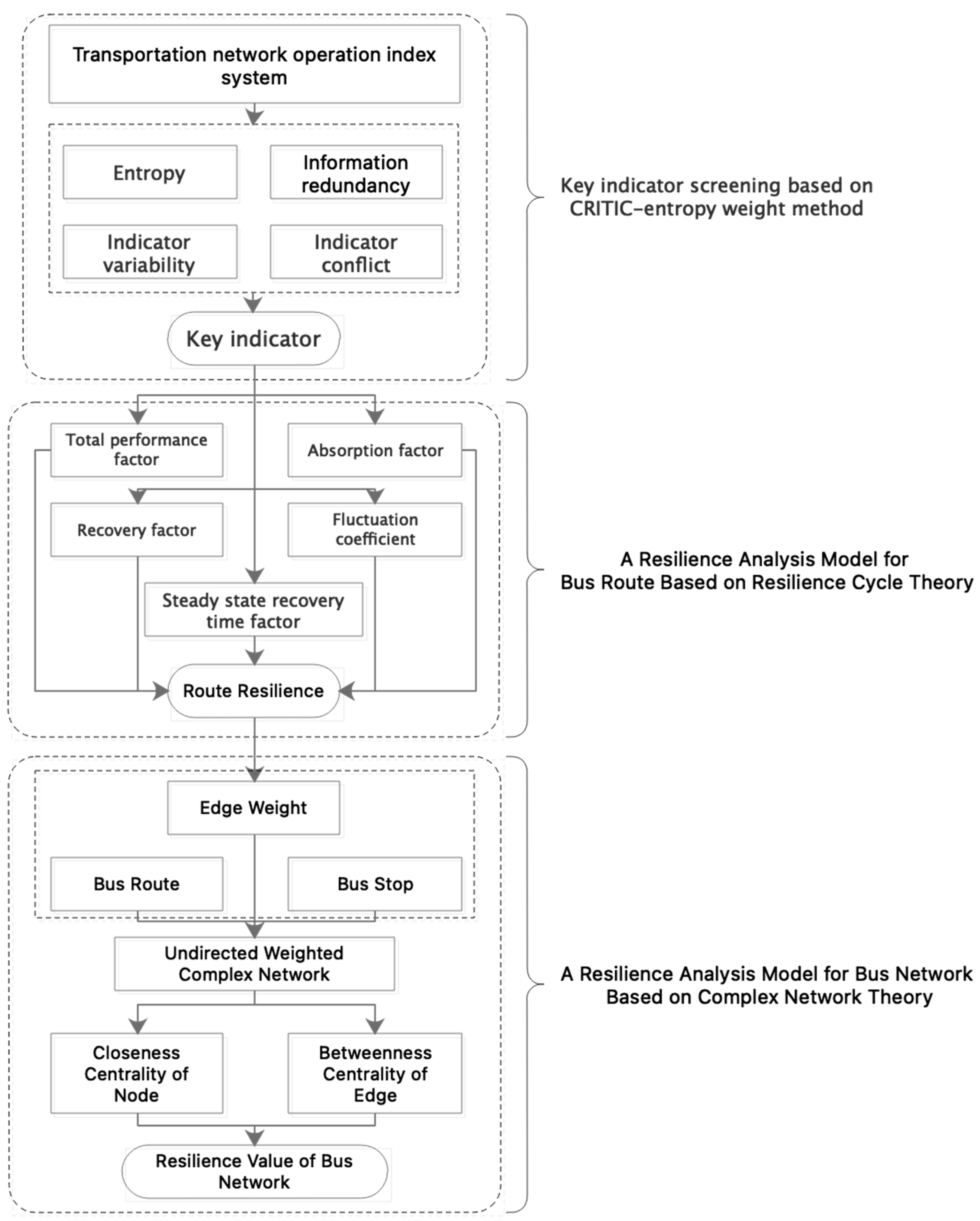
As shown in Figure 5, in the context of studying the dynamic characteristics of bus route systems and the static structure of bus networks, this paper defines the resilience of a bus network as its ability to resist, reduce, and absorb the impact of disturbances (such as shocks, interruptions, or disasters), maintain an acceptable level of service (static resilience of the transportation network structure), and restore normal and balanced operation within a reasonable time and cost (dynamic resilience of the transportation network in terms of time and space). The performance of bus routes is the external manifestation of the working state of the network. To quantify the performance of the bus network, performance indicators must be relied upon, such as the average speed of a route, passenger flow, and one-way travel time to express route performance. To determine the most representative performance indicators, it is necessary to screen the existing monitoring indicators for bus network operation and obtain key indicators that fully reflect the status of the bus network.

Figure 5. Research approach.

This paper first uses the CRITIC–entropy method to objectively determine the key indicators for analyzing the resilience of bus routes. Then, the changes in key indicators during the resilience cycle are taken as an expression of system performance, and a bus route resilience analysis model based on resilience cycle theory is proposed to quantify the absorption capacity, degree of performance decline, and recovery ability of bus routes in the face of unexpected events. Performance factors, absorption factors, recovery factors, steady-state recovery time factors, and fluctuation coefficients are defined for each stage of the resilience cycle, and bus route resilience is determined based on these resilience calculation factors. The resilience value of a route is a comprehensive reflection of its robustness and resistance to destruction when facing unexpected events, and the higher the resilience value of a route, the less likely it is to be affected by unexpected events. Finally, based on complex network theory, the resilience of the bus network is analyzed using the closeness centrality and edge betweenness centrality of the complex network to quantify the resilience value of the bus network in a static state. On this basis, the centrality index of the network is weighted by the resilience value of the bus route, so that the constructed model not only considers the static network structure but also takes into account the dynamics of bus routes.

3.2. Transport Network Index Evaluation Model Based on CRITIC–Entropy Weight

This article uses a combination evaluation model to construct an indicator evaluation algorithm suitable for this study. The combination evaluation model is a method of weighting and combining multiple single evaluation models to integrate the advantages of single evaluation models. The data of the indicator system for monitoring and analyzing the operation status of the public transportation network in this article are all based on real quantitative data of the public transportation network operation, and there are no qualitative indicators that cannot be explained or calculated. Therefore, there is no need to use evaluation methods that combine qualitative and quantitative analysis, such as expert experience method or analytic hierarchy process.

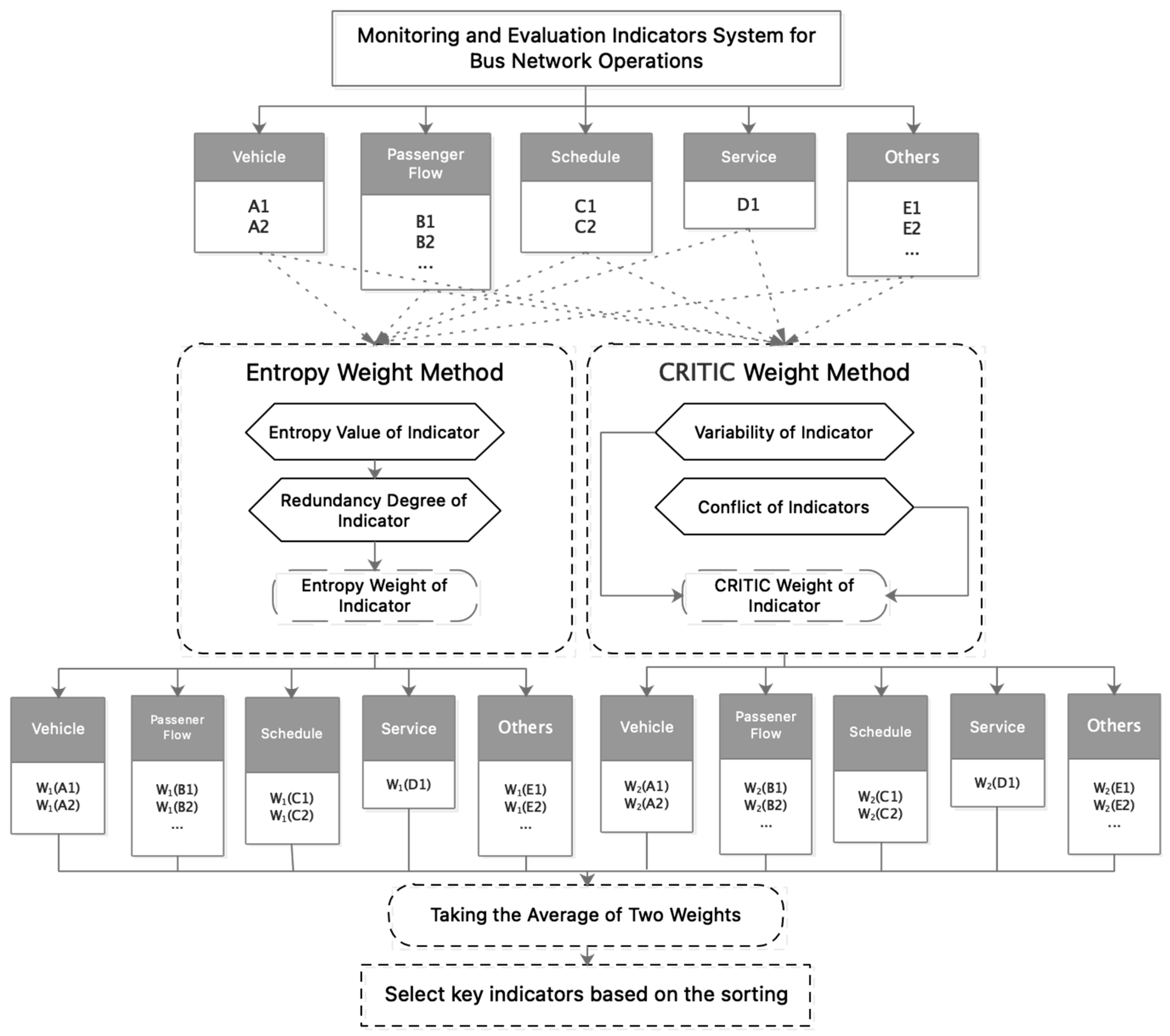
This study improved upon existing objective weighting methods, such as fuzzy comprehensive evaluation, entropy weighting, TOPSIS, and CRITIC (criteria importance through inter-criteria correlation), by combining entropy weighting with CRITIC to compensate for CRITIC’s inability to consider the discreteness of attribute values. CRITIC emphasizes the comparability and conflict of indicators and calculates the objective weights of indicators based on these attributes, but it does not consider the discreteness of attribute values. In contrast, entropy represents the degree of disorder of a system, and the smaller the entropy value of an indicator value, the more information it contains and the higher the weight, making it more capable of reflecting the operational characteristics of the bus network. The combination of entropy weighting and CRITIC in this study resulted in a CRITIC–entropy weighting model for selecting key indicators, as shown in Figure 6.

Figure 6. CRITIC–entropy weight method.

The steps for using the entropy weight method to select key indicators are as follows:

(1) Select $n$ samples and $m$ indicators within a time period affected by a sudden event. Then $x_{ij}$ represents the value of the $j$ indicator for the $i$ sample $\left(i=1,2,\dots ,n;j=1,2,\dots ,m\right)$.

(2) Homogenize the indicators: Homogenize the heterogeneous indicators to facilitate subsequent calculations. Since the calculation units of each indicator in the indicator system are not unified, using them directly will affect subsequent calculations. Therefore, before calculating the indicator weights, the data of each indicator needs to be standardized, unified, and homogenized. The absolute value of each indicator is used to solve the homogenization problem (i.e., $x_{ij}=\left|x_{ij}\right|$). In addition, the indicator system contains both positive indicators (max-type indicators) and negative indicators (min-type indicators), with different numerical meanings (higher values are better for positive indicators, while lower values are better for negative indicators). Therefore, different algorithms are used to standardize data for positive and negative indicators. The specific methods are as follows:

$$\max \text{-}\mathrm{type}\mathrm{indicators}:x_{ij}{}^{’}=\frac{x_{ij}-min\left\{x_{1j},\dots ,x_{nj}\right\}}{max\left\{x_{1j},\dots ,x_{nj}\right\}-min\left\{x_{1j},\dots ,x_{nj}\right\}}$$

(1)

$$\min \text{-}\mathrm{type}\mathrm{indicators}:x_{ij}{}^{’}=\frac{max\left\{x_{1j},\dots ,x_{nj}\right\}-x_{ij}}{max\left\{x_{1j},\dots ,x_{nj}\right\}-min\left\{x_{1j},\dots ,x_{nj}\right\}}$$

(2)

To simplify the expression, let $x_{ij}=x_{ij}{}^{\prime }$;

(3) Calculate the weight $p_{ij}$ of the $i$ sample value under the $j$ indicator:

$$p_{ij}=\frac{x_{ij}}{{\sum }_{i=1}^n{x}_{ij}}$$

(3)

(4) Calculate the entropy value $e_j$ for the $j$ indicator:

$$e_j=-k{\sum }_{i=1}^n{p}_{ij}\ln \left(p_{ij}\right)$$

(4)

Here, $k=\frac{1}{\ln \left(n\right)}>0$ satisfies $e_j>0$.

(5) Calculate the redundancy degree of information entropy $d_j$:

$$d_j=1-e_j$$

(5)

(6) Calculate the entropy weight of each indicator $w_j{}^{\left(1\right)}$:

$$w_j{}^{\left(1\right)}=\frac{d_j}{{\sum }_{j=1}^m{d}_j}$$

(6)

(7) Calculate the variability of each indicator, represented by the standard deviation $S_j$:

$$\left\{\begin{array}{c}{\overline{x}}_j=\frac{1}{n}{\sum }_{i=1}^n{x}_{ij}\\ S_j=\sqrt{\frac{{\sum }_{i=1}^n{\left(x_{ij}-{\overline{x}}_j\right)}^2}{n-1}}\end{array}\right.$$

(7)

In the CRITIC method, the standard deviation is usually used to calculate the indicator weights. The idea is to reflect the information contained in the indicators based on the fluctuation of the numerical differences within the indicators. The greater the fluctuation of the numerical differences, the higher the evaluation intensity of the indicator. The fluctuation of the numerical differences can be quantified by the standard deviation. Therefore, indicators with larger standard deviations will have higher weights in the CRITIC method.

(8) Calculate the indicator conflict $R_j$. The indicator conflict reflects the correlation between indicators. The smaller the correlation, the greater the conflict of the indicators. Generally, indicators with high conflict can reflect more information. Indicators with higher correlation have higher redundancy and less reference value. Therefore, indicators with higher conflict often have higher evaluation weights. The calculation of indicator conflict $R_j$ utilizes the Pearson correlation coefficient. Here, $r_{ij}$ represents the average Pearson coefficient of indicator $j$ with other indicators in the $i$ sample, reflecting the correlation of indicator $j$ with other indicators. The calculation of indicator conflict is shown in the formula.

$$R_j={\sum }_{i=1}^n\left(1-r_{ij}\right)$$

(8)

(9) Calculate the CRITIC weight of each indicator $w_j{}^{\left(2\right)}$:

$$w_j{}^{\left(2\right)}=\frac{S_j\times R_j}{{\sum }_{j=1}^m{S}_j\times R_j}$$

(9)

(10) The CRITIC method has the advantage of considering the strength of the indicators’ contrast and the correlation between data, while the entropy weight method indirectly reflects the importance of indicators based on the degree of dispersion. In order to complement the advantages of these two weighting methods, this study combines and improves the two methods, assuming that they have equal status, and constructs a key indicator evaluation model based on the CRITIC and entropy weight methods. Thus, it achieves the objective of taking the strengths of both weighting methods and calculating the total weight of each indicator $w_j$, as shown in the formula:

$$w_j=\frac{w_j{}^{\left(1\right)}+w_j{}^{\left(2\right)}}{2}$$

(10)

The total weights $w_j$ calculated based on the established CRITIC–entropy weight evaluation model are sorted to obtain the key indicators used to calculate the resilience of the bus network.

3.3. Transport Lines Resilience Analysis Model Based on Resilience Theory

The resilience of bus routes mainly focuses on reflecting the dynamic resilience of the bus network system, which refers to the ability of the line performance to gradually degrade and recover to a steady state before the disturbance when the public transportation network system is interfered with due to sudden events such as traffic accidents, natural disasters, large-scale social activities, etc. The occurrence of sudden events in the environment where bus routes are located is a prerequisite for the disturbance of the bus network. The performance of bus routes is the external manifestation of the network operation status. For example, the line performance can be represented by the average speed of the line, passenger volume, and one-way running time of the line. The sudden event changes the network performance by affecting the working status of the bus routes themselves. Therefore, this section analyzes the resilience of bus routes by using the key indicators obtained in the previous section as the line performance. Based on the resilience cycle theory, a resilience analysis model is constructed by analyzing the change curve of the key indicators under the impact of sudden events.

• Model construction.

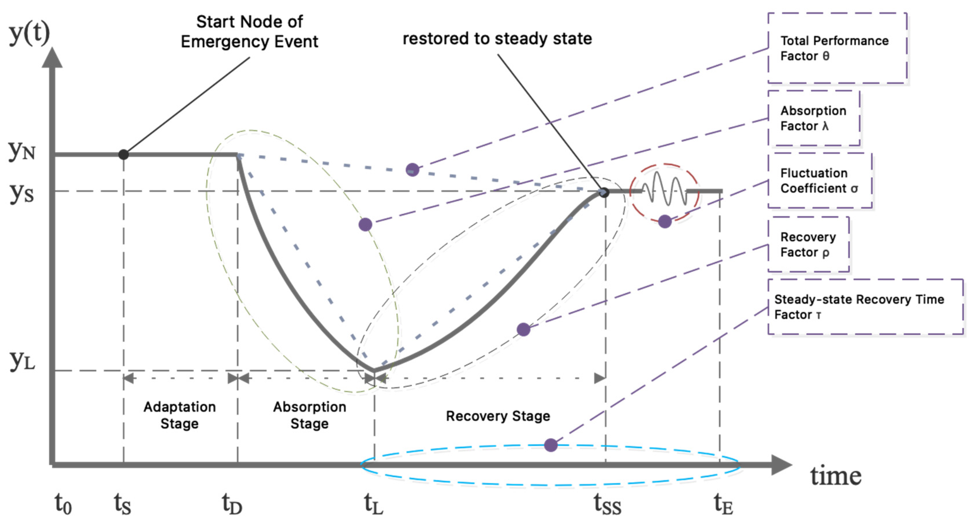
As shown in Figure 7, in the event of a sudden incident, the performance indicators of a bus route usually exhibit a trend of initially declining and then rebounding over time. In existing resilience research, the resilience cycle theory is typically used to segment this trend, with the adaptation phase being from the start of the incident until the system performance begins to decline, the absorption phase being from the start of system performance decline until it reaches the lowest point, and the recovery phase being from the start of system performance recovery until it reaches the expected stable level.

Figure 7. Resilience analysis of bus routes (y-axis: indicator value).

The Y-axis represents the measurement of public transit performance over time. $t_S$ represents the time when the sudden event occurs, while $t_D$ represents the time when the transit system performance starts to decline. In general, $t_S$ is not equal to $t_D$, because the change caused by the sudden event and the spread of negative effects may delay the decline of performance. For example, the impact of a traffic accident on a bus route may not be evident until congestion or traffic control measures appear, while a relatively major sudden event, such as a natural disaster, can quickly bring negative effects to the transit system. $t_L$ represents the time when the transit system performance reaches its lowest point, and $t_{SS}$ represents the time when the transit system performance stabilizes again. According to the resilience cycle theory, the resilience response of a public transit route can generally be divided into three stages after a sudden event occurs: first is $t_S\to t_D$, where due to the absorption capacity of the route’s resilience, the decline in performance caused by the sudden event is not immediately apparent. Second, is $t_D\to t_L$, during which the decline in performance caused by the sudden event will reach its maximum, and the peak value of performance decline is determined by the route’s adaptation capacity. Finally, $t_L\to t_{SS}$, which is the recovery stage of the route’s resilience, where the system performance will gradually recover to the stable level before the sudden event occurred, and the recovery rate is determined by the route’s recovery capacity.

The resilience of public transit routes in these three stages is difficult to measure using a single dimension. Therefore, a unified quantitative research method is proposed to comprehensively evaluate the resilience of public transit routes in response to various unexpected events. Thus, the resilience of public transit routes can be further summarized as the ability to eliminate negative impacts before unexpected events occur, adapt to impacts after the events, and recover from the damage and changes brought about by the events. Based on the above research foundation, this study quantifies the abilities of the three stages of resilience (adaptation, absorption, and recovery) and forms calculation factors to calculate the resilience of the route. The calculation factors fully consider the changes in the resilience cycle. The public transit route resilience analysis model proposed in this study, based on the resilience cycle theory, is defined as follows:

Firstly, a resilience indicator $R_L$ is defined to quantify the overall resilience of a public transit route within a resilience cycle that has been impacted by an unexpected event. Based on the definition of the resilience hypothesis, important features are determined to quantify the overall resilience indicator in the resilience calculation process. These important features are quantified by a set of resilience factors, which are used to calculate the overall resilience of the public transit route, as shown in the equation.

$$R_L=\left\{\begin{array}{c}\theta \rho \left[\lambda +\sigma +1-{\tau }^{\left(\rho -\lambda \right)}\right] if \rho -\lambda \ge 0\\ \theta \rho \left(\lambda +\sigma \right) otherwise\end{array}\right.$$

(11)

In the calculation of the overall resilience capability index of the bus route, $\theta$ is a resilience quantification factor that can generally reflect the resilience changes in a complex system. However, in order to make the calculation of route resilience more sensitive to the resilience period under the impact of sudden events, we optimize this resilience calculation method by integrating a set of resilience factors. Among them, the recovery factor $\rho$ reflects the system’s final recovery state (i.e., its recovery performance) and reflects the system performance changes in the recovery stage of the resilience period. The absorption factor $\lambda$ reflects the system’s ability to absorb the impact of sudden events and reflects the system performance changes in the absorption stage of the resilience period. The volatility factor $\sigma$ explains the volatility of indicator data, representing the system’s ability to smoothly transition from one state to another. Due to the general data fluctuations in various indicators of the bus route, the volatility factor $\sigma$ can reduce the interference caused by data fluctuations. The normalized recovery time factor $\tau$ represents the system’s response speed by the time required to reach a steady state after being affected by sudden events. For the discrete indicator time series data in this study, $\tau$ can be defined as the ratio of the observed number of the system in the steady state to the total number of observations. The influence of $\tau$ decreases with the decrease in the indicator recovery amount (i.e., $\rho -\lambda$). The conditional statement in the formula ensures that the bus route can only reach a steady state quickly (i.e., with a low $\tau$ value) when its recovery performance is better than its absorption performance. Only one $R_L$ value is calculated within a resilience period (i.e., $R_L$ is a function of the time interval from $t_S$ to $t_E$, not directly a function of time t).

The following introduces the definition of each resilience quantification factor in the resilience calculation formula for bus routes.

(1)

Overall performance factor $\theta$

The overall performance factor $\theta$ reflects the system’s resilience in a complete resilience cycle affected by sudden events, and its calculation formula is:

$$\theta =\frac{{\int }_{t_S}^{t_E}y\left(t\right)dt}{(t_E-t_S)y_N}$$

(12)

Under normal circumstances, the value of $\theta$ is [0,1], and when the system performance does not decrease, $\theta$ is 1. This indicator reflects the resilience capability during a complete period. This calculation method is also applied to the resilience of other complex systems. Although it can measure the resilience of a system in normal application scenarios, its shortcomings are also obvious. Its calculation result does not reflect the changes in the system during the absorption and recovery stages. For example, there are two systems A and B. When encountering sudden events, system A suffers a severe performance decline but recovers quickly, while system B has a slight decline in performance but recovers slowly. Using θ to calculate the system’s resilience may result in the same value. The fundamental reason is that θ does not take into account the absorption rate, recovery rate, and data volatility of the bus network. Therefore, we need to incorporate other resilience quantification factors to identify the system’s absorption rate, recovery rate, and data volatility.

(2)

Absorption factor λ

Quantifying the ability of a bus route to absorb the impact of unexpected events is crucial. The absorption factor $\lambda$ represents the ability of the system to absorb the impact of unexpected events on system performance, reflecting the absorption capacity of the route during the resilience cycle. Its calculation formula is:

$$\lambda =\frac{y_L}{y_N}$$

(13)

$\lambda$ usually takes a value between 0 and 1 and is 1 under normal circumstances. The absorption factor can reflect the ability of the system to absorb negative impacts when facing unexpected events, and the smaller the value, the greater the degree of impact on the system.

(3)

Recovery factor ρ

The calculation formula used to quantify the recovery capacity of bus routes during the resilience period is:

$$\rho =\frac{y_S}{y_N}$$

(14)

where $0\le \rho \le \infty$, and $y_S$ is the stable value of system performance after recovery. In this study, the commonly used augmented Dickey–Fuller (ADF) test in time series analysis was used to determine when the bus route reached stationarity, i.e., to determine $t_{SS}$ and $y_S$. For bus route indicators with obvious daily trends (morning and evening peak periods) and data drift, an autoregressive process with drift and trend terms was used for ADF testing, as shown in equation:

$$Y_t=\omega +\beta t+\gamma Y_{t-1}+{\sum }_{i=t_L}^k{C}_i\Delta Y_{t-i}+{\epsilon }_t,Y_0=0$$

(15)

where $\omega$ is the constant term, $\beta t$ is the time trend, ${\epsilon }_t$ is the random disturbance term, and t takes values from [$t_L,t_E$]. The hypothesis is that there is a unit root in the time series, making it non-stationary for the null hypothesis, and the alternative hypothesis is that there is no unit root, indicating that the time series is stationary with an intercept and trend. If we strictly judge whether the sequence is weakly stationary, we can directly test whether it is stationary without intercept and trend. If the null hypothesis cannot be rejected (e.g., p > 0.05), the sequence is non-stationary, and it is still necessary to test whether the sequence is trend stationary.

(4)

Steady-state recovery time factor $\tau$

The steady-state recovery time factor $\tau$ is used to capture the speed at which the system recovers to a steady state during the recovery phase of the resilience cycle. This factor considers the recovery capacity of the bus route when preventive measures are taken.

$$\tau =\frac{t_{SS}-t_L}{t_E-t_S}$$

(16)

where $0\le \tau \le 1$ and approaches 0 under normal circumstances.

(5)

fluctuation coefficient $\sigma$

The fluctuation coefficient σ is used to address the highly unstable performance data of the bus routes. This study borrows the concept of signal-to-noise ratio from communication system research, which originally refers to the ratio of signal to noise in an electronic device or system. In this study, the trend in bus route indicators is analogous to the signal in an electronic system, while the data fluctuation is analogous to the noise. Thus, the fluctuation of the system performance data is quantified using the signal-to-noise ratio ($SN{R}_{dB}$) and represented by the fluctuation factor $\sigma$. The role of the $\sigma$ coefficient is to reduce the error caused by data fluctuations in resilience calculations.

$$SN{R}_{dB}=10lg\frac{{\sum }_{t=t_S}^{t_E}{y}_{raw}{\left(t\right)}^2}{{\sum }_{t=t_S}^{t_E}n{\left(t\right)}^2}$$

(17)

The numerator is calculated from the original bus route data, and the denominator is the noise data obtained by subtracting the smooth data from the original data, as shown in equation:

$$n_{\left(t\right)}=y_{raw}\left(t\right)-y_s\left(t\right)$$

(18)

Using logical functions to convert $SN{R}_{dB}$ is converted to the volatility factor, and the conversion formula is shown in equation:

$$\sigma =\frac{1}{1+exp\left[-0.3\left(SN{R}_{dB}-10\right)\right]}$$

(19)

where $0\le \sigma \le 1$, and the value is 1 when there is no influence from unexpected events. The setting of the function slope (set to −0.3) and the offset (set to 10) accurately allows observation of data fluctuations. As the data fluctuation increases, $\sigma$ gradually decreases.

2.

Model validation

In order to provide a reference for comparison with the model proposed in this study, this section uses the resilience calculation method commonly used in resilience research to calculate the resilience indicators for comparison. The calculation method is as follows:

$$R_C=\frac{{\int }_{t_S}^{t_E}y\left(t\right)dt}{{\int }_{t_S}^{t_E}{y}_{N}dt}$$

(20)

To simplify the model validation process, we construct the following function $y\left(t\right)$ to make the data exhibit the resilience periodic characteristics of public transportation indicators when encountering sudden events:

$$y\left(t\right)=\left\{\begin{array}{c}\frac{m_1-l}{\exp \left[r_1\left(t-p_1\right)\right]+1}+l+n t\in \left[0, 50\right], n\in N\left(0,{\sigma }^2\right)\\ \frac{m_2-l}{\exp \left[-r_2\left(t-p_2\right)\right]+1}+l+n t\in \left[50, 100\right], n\in N\left(0,{\sigma }^2\right)\end{array}\right.$$

(21)

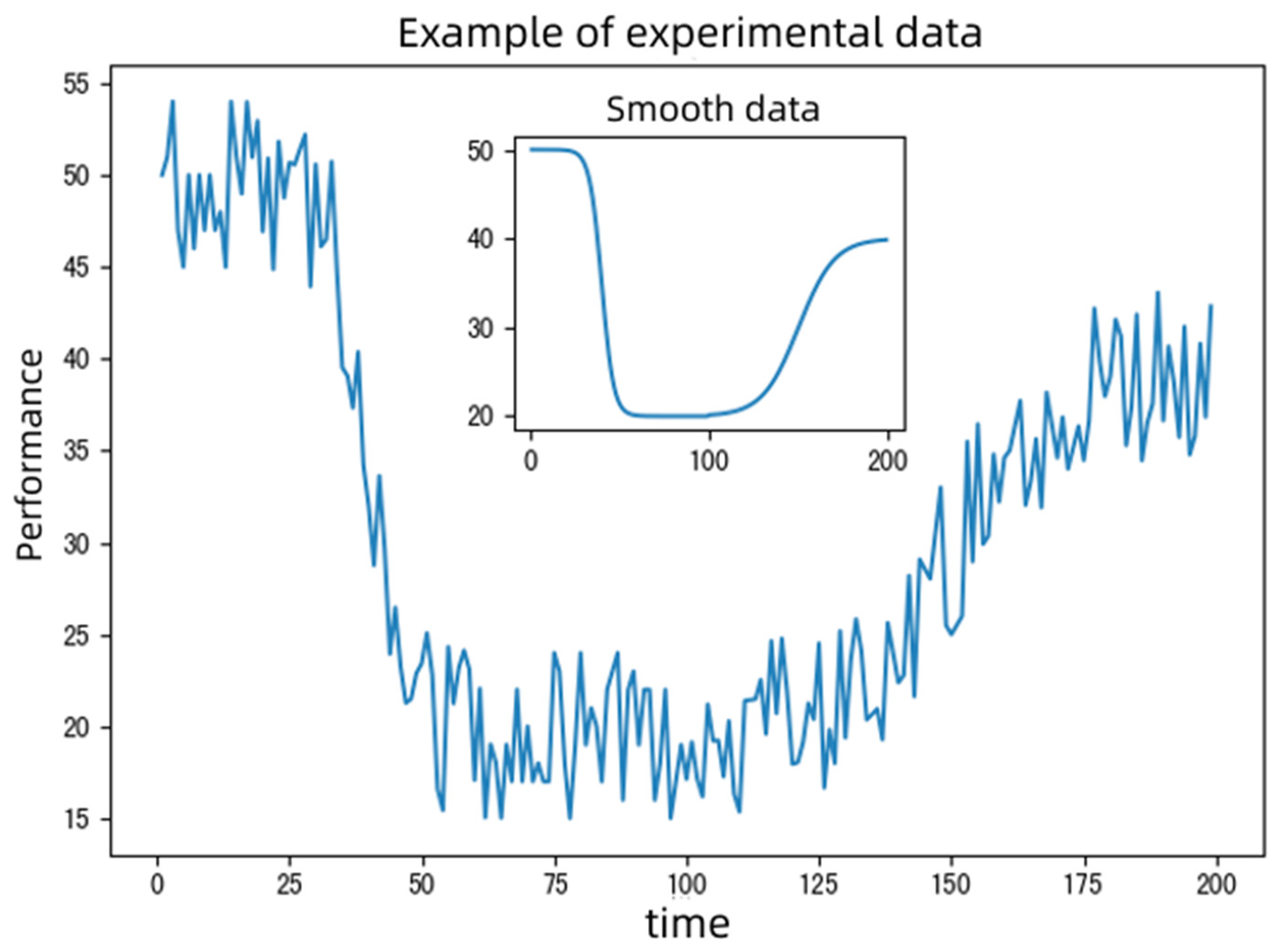
where $m_1$ is the initial value, $m_2$ is the final stable value, $l$ is the minimum value, $r_1$ and $r_2$ are the slope coefficients for the decrease and increase, respectively, and $p_1$ and $p_2$ are the midpoints for the decrease and increase processes. $n$ represents data noise that follows a normal distribution with mean 0 and standard deviation $\sigma$. These parameter variations simulate the changes in the performance of different systems during the resilience cycle, such as the maximum and minimum values, stable values, and rates of decrease and recovery. The ultimate goal is to compare the accuracy of two resilience calculation methods under different parameters. The data generated by the above function with parameters $m_1=50$, $m_2=40$, $r_1=0.3$, $r_2=0.07$, $p_1=40$, $p_2=150$, $l=20$, and $\sigma =5$ is shown in Figure 8.

Figure 8. Data of model validation.

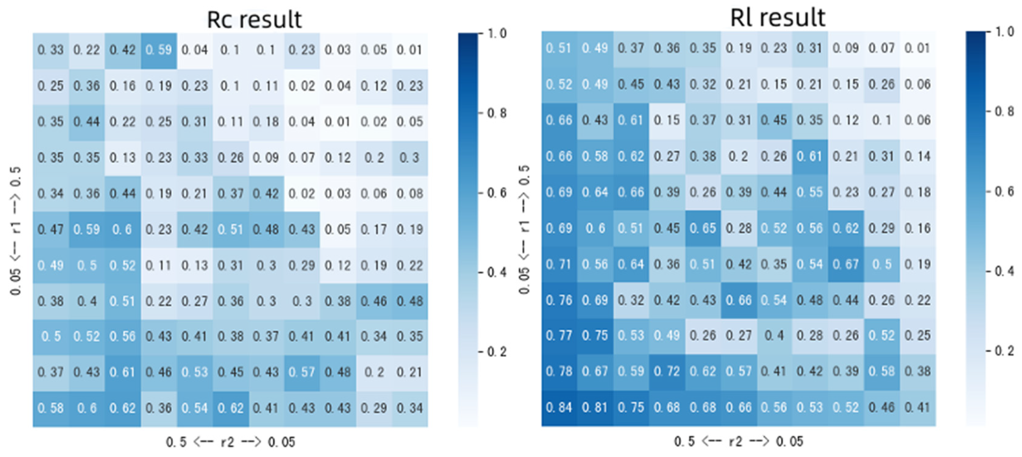
Because $r_1$ and $r_2$ reflect the data’s decline and recovery rates, they represent to some extent the absorption and recovery capacity of the bus route during the resilience period. To verify which model is more sensitive to these two capabilities, the two rates can be taken in the range of (0.05, 0.5), and the resilience values based on the two models can be calculated separately. The calculation results are shown in Figure 9.

Figure 9. Model verification results.

Observing the results of the model calculations, it can be seen that as $r_1$ decreases and $r_2$ increases, the system resilience gradually improves. This simulates that the improvement of the absorption and recovery capabilities during the absorption and recovery stages in the resilience period can enhance system resilience. However, from the comparison of the data heatmap, the color blocks of the $R_l$ model data are relatively more concentrated, indicating that the $R_l$ model is more sensitive to changes in $r_1$ and $r_2$. Although the $R_C$ model can also capture this trend of change, its sensitivity is not as good as $R_l$, and its heatmap color blocks are relatively scattered. The experimental results show that the line resilience analysis model based on the resilience cycle theory proposed in this study calculates the system resilience more accurately and is more sensitive to changes in resilience absorption and recovery stages.

3.4. Transport Network Resilience Analysis Model Based on Complex Network

From the perspective of static resilience in the definition of this article, the basic service function of the bus network is to transport passengers from one station to another. When a sudden event interrupts the connection between two stations, the most effective method is to choose another bus route that connects the two stations. Therefore, the recovery of the transportation function between two stations largely depends on whether there are alternative paths besides the normal path. In short, based on the definition of resilience in this article, if the bus network can provide more shortest paths to reach the destination in the event of a sudden event, then the bus network has a relatively high resilience value. W.H. Ip et al. proposed a similar definition of resilience, defining it as the number of reliable routes between any two nodes, to calculate the ability to restore transportation function after partial road closure [51].

From the perspective of complex networks, the resilience of a bus network can be evaluated by the weighted average of centrality indicators of the bus network’s stations and routes. Based on this idea, this study abstracts the bus network into a weighted complex network similar to a BA scale-free network. Nodes and edges are important components of complex networks, and analyzing their importance is a key approach to analyzing complex networks. In general, centrality measures such as degree centrality are commonly used to analyze the importance of nodes and edges in a network. Nodes and edges that have a greater impact on the structure and function of the entire network are generally more important. Although these important nodes and edges are relatively few in number, their influence can quickly spread throughout the entire network. Given the need to analyze the resilience of the bus network in this study, identifying the importance of network nodes and edges becomes the first problem to be solved. There are currently many different methods for calculating network node centrality, including degree centrality, betweenness centrality, closeness centrality, and eigenvector centrality. Degree centrality reflects the degree of centralization or concentration of the network and is suitable for situations where the entire network operates around a set of core nodes. Betweenness centrality is developed around the concept of betweenness and can measure the information transmission ability of a node or edge. The calculation method for betweenness centrality involves counting the number of times the shortest path passes through a node. Nodes with high betweenness centrality, like transportation hubs, bear a large information transmission task. Closeness centrality reflects the size of the average distance between the selected node and other nodes in the network. The smaller the average distance, the more central the node is in the network. The definition of closeness centrality is the reciprocal of the average length of the shortest path between the node and all other nodes in the network. Based on this, this study proposes a bus network resilience analysis model based on node closeness centrality and edge betweenness centrality, as shown in Figure 10.

Figure 10. Public transit network resilience analysis model.

To facilitate the description of the model’s calculations, this study introduces the mathematical symbols shown in Table 1:

Table 1. Mathematical symbol definition.

Mathematical Symbols	Meaning
$G=\left\{V,E\right\}$	Scaleless weighted network of public transport network
$V$	Collection of nodes
$E$	Set of edges
$n$	Number of nodes
$m$	Number of edges
$v_i i=1,2,\dots ,n$	Node $i$
$e_l l=1,2,\dots ,m$	Edge $l$
$k_i$	Node degree
$e_{ij}\in E$	$\mathrm{Edge}\mathrm{of}{v}_i$ $\mathrm{and}{v}_j$
$w\left(e_{ij}\right)$	$\mathrm{Weight}\mathrm{of}{e}_{ij}$, is the normalized line resilience value
$d_{ij}$	$\mathrm{Distance}\mathrm{of}{v}_i$ $\mathrm{and}{v}_j$
$N_i$	$\mathrm{The}\mathrm{set}\mathrm{of}\mathrm{adjacent}\mathrm{points}\mathrm{of}{v}_i$

According to this study’s definition of bus network resilience based on network recovery capacity and the characteristics of weighted scale-free networks, the resilience of a bus network is defined as follows:

$$R_{total}=(\frac{{\sum }_{i=1}^{n}C\left(v_i\right)}{n}+\frac{{\sum }_{l=1}^{m}B\left(e_l\right)}{m})/2$$

(22)

where $\mathrm{C}\left(v_i\right)$ is the normalized value of the weighted value $C_C{}^{\prime }\left(v_i\right)$ based on the closeness centrality of the $v_i$ node, which can be considered as the resilience value of the node. The normalization formula is:

$$C\left(v_i\right)=\frac{C_C{}^{’}\left(v_i\right)-C_C{}^{’}{\left(v_i\right)}_{min}}{C_C{}^{’}{\left(v_i\right)}_{max}-C_C{}^{’}{\left(v_i\right)}_{min}}$$

(23)

$C_C{}^{\prime }\left(v_i\right)$:

$$C_C{}^{’}\left(v_i\right)={\sum }_{i=1,j\ne i}^n\frac{S_i\left(n-1\right)}{d_{ij}\times k_i}$$

(24)

$$S_i={\sum }_{j\in N_i}w\left(e_{ij}\right)$$

(25)

The weight used in $C_C{}^{\prime }\left(v_i\right)$ is the unit weight of the node, i.e., $S_i/k_i$, where the unit weight of a node is the sum of the weights of edges connected to the node divided by its degree, which reflects the weight of edges around the node. Referring to the concept of closeness centrality, the average distance between each node and other nodes is calculated, and for a given node, the higher the closeness centrality, the more central it is in the network.

4. Case Analysis

4.1. Description of Usage Data

(1)

Data for filtering key indicators

The data used in the experiment comes from the statistical data provided by the Beijing Traffic Operation Monitoring and Dispatching Center, an authoritative institution in Beijing. The data quality is relatively high. There are 12 datasets used in the case analysis: actual departure interval, actual arrival interval, passenger volume, card swipe volume of stations on the route, occupancy rate, OD passenger flow, on-time departure rate, online operating vehicles, station punctuality rate, one-way travel time, instances of bus bunching, instances of long interval, which form the indicator system shown in Table 2.

Table 2. Bus operation monitoring index system.

Indicator Criteria Layer	Indicator Name	Indicator Define
Vehicle (A)	Actual departure interval (A1)	The time interval between two adjacent buses on the same route departing from the starting station
	Actual arrival interval (A2)	The average actual arrival time of two adjacent bus trips on the same route
Passenger flow (B)	Card swiping passenger volume (B1)	Number of passengers using the bus card to swipe their cards
	Landing volume (B2)	The number of boarding and alighting passengers of bus operating vehicles at the station
	Load factor (B3)	The ratio of actual passenger capacity to rated passenger capacity
	OD passenger flow (B4)	Average traffic volume between the starting and ending points
Schedule (C)	On schedule departure rate (C1)	The percentage of scheduled on-time departures in the total number of departures during the statistical period
	Number of online operating vehicles (C2)	Number of real-time vehicles used for operational business
Service (D)	Punctuality rate (D1)	The probability of public transportation vehicles arriving at a certain station on schedule during the statistical period
Others (E)	Bus single-trip time (E1)	The actual time from the initial station to the final station for public transportation vehicles
	Bunching (E2)	The number of occurrences where the interval between adjacent bus arrivals at each station is less than 1 minute
	Big interval (E3)	The number of times the arrival interval of adjacent buses at each station is greater than 15 min

To facilitate an accurate evaluation based on the patterns contained in each indicator during the cycle, the selected time range is from 10 to 16 August 2020, a total of one week. The data are collected at an hourly granularity, and there was heavy rain on August 12. Before using the data, it is necessary to check and process redundant data, missing values, and outliers. The necessary data filtering conditions are shown in Table 3.

Table 3. Data filtering condition-filtering key indicators.

Condition	Value
Date	10–16 August 2020
Bus line	line 1 (East-west), line 139 (north-south)
Operation time	00:00–23:00
Time granularity	1 h
Running direction	0/1
Ascending/descending	Ascending, descending, ascending and descending

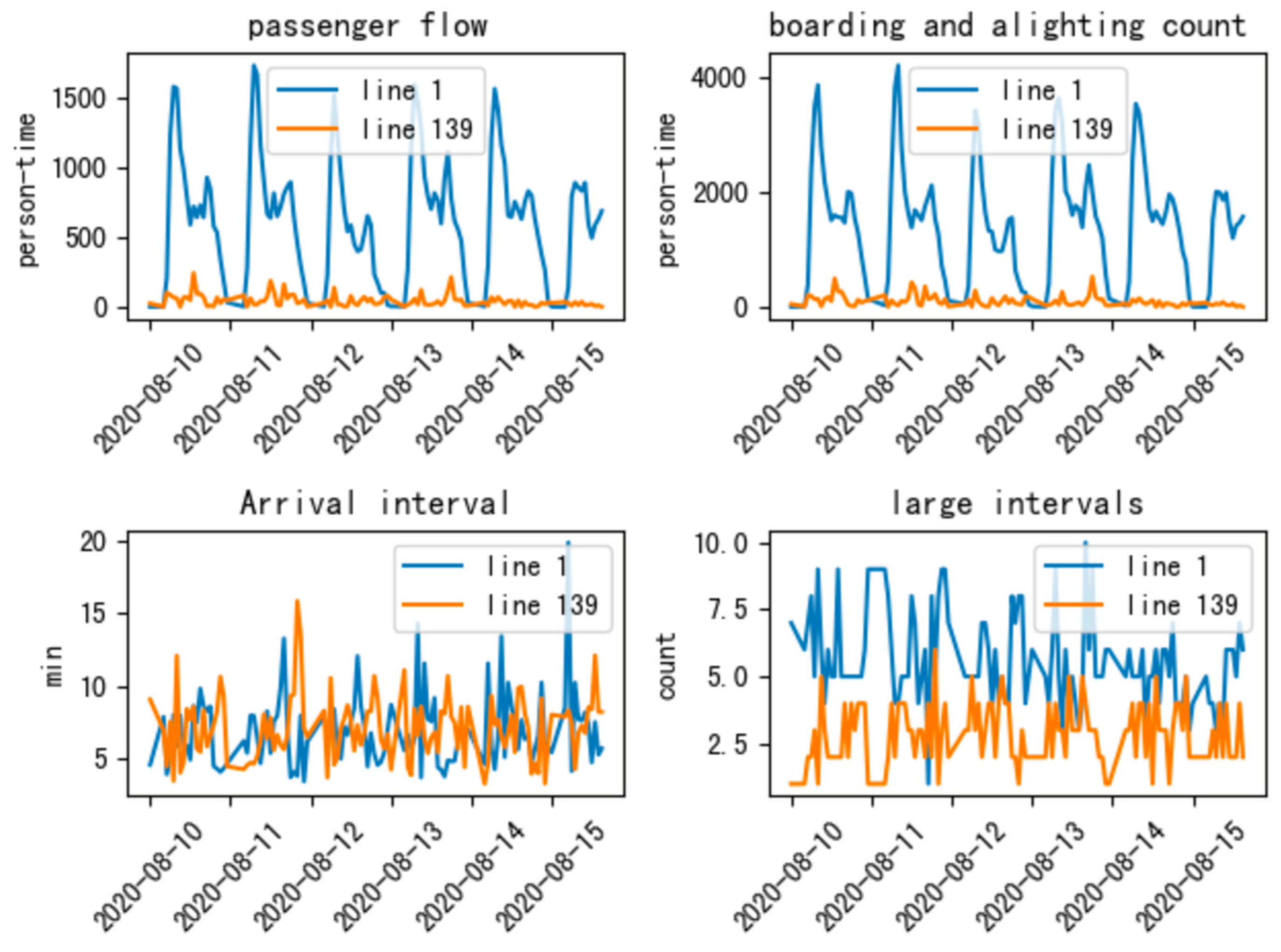
The trend comparison of some data is shown in Figure 11:

Figure 11. Trend of indicators (y-axis: indicator value).

(2)

Data for bus route resilience analysis

The example analysis utilizes two datasets: “Card Swiping Entries and Exits at Route Stations” and “Card Swiping Passengers on the Route.” Before using the data, it is necessary to check and process redundant data, missing values, outliers, etc. The necessary data filtering conditions are shown in Table 4.

Table 4. Data filtering condition-bus route resilience analysis.

Condition	Value
Date	10–16 August 2020
Bus line	Line 1, Line 139, Line 101, Line 116, Line 2, Line 40, Line 60
Bus stop	Line 58 (Sihui Hub Station-Forbidden City Station)-17 stations
Operation time	00:00–23:00
Time granularity	1 h
Running direction	0/1
Ascending/descending	Ascending, descending, ascending and descending

Below is a presentation of some data:

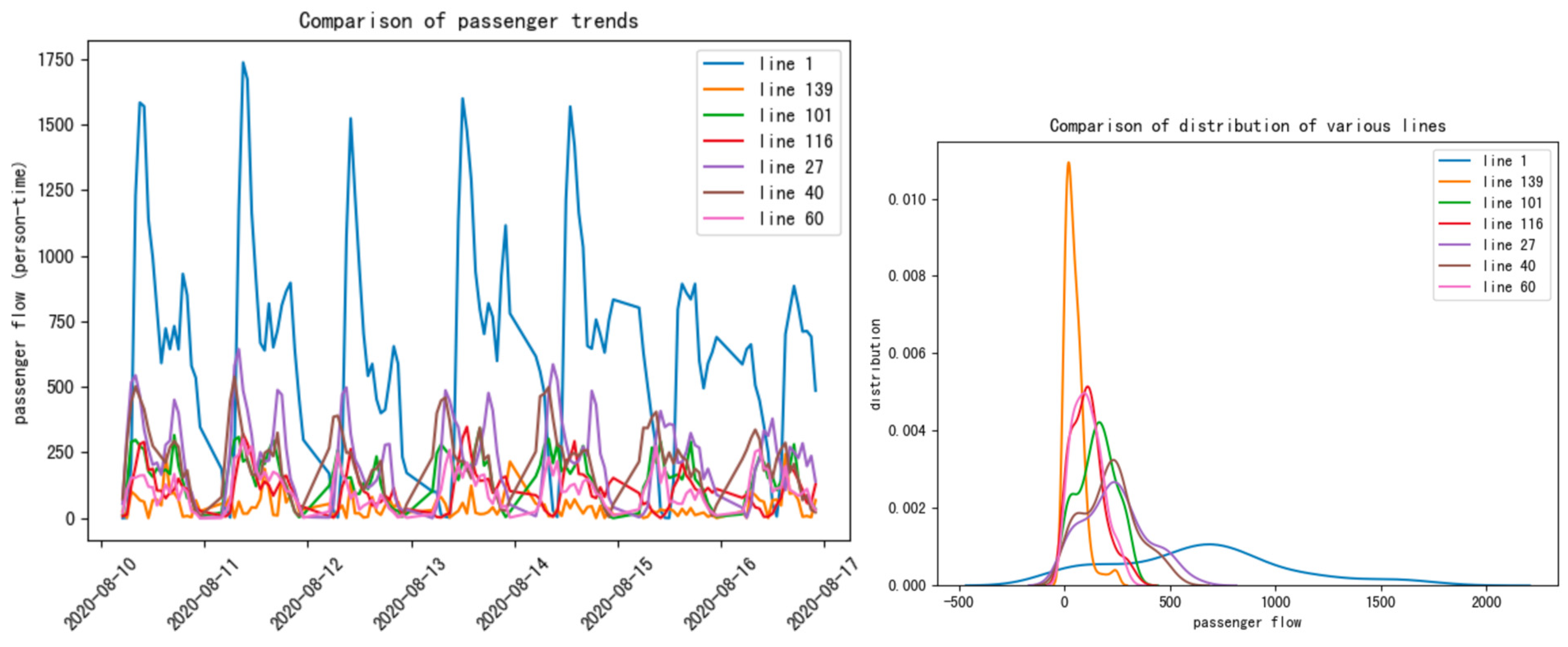
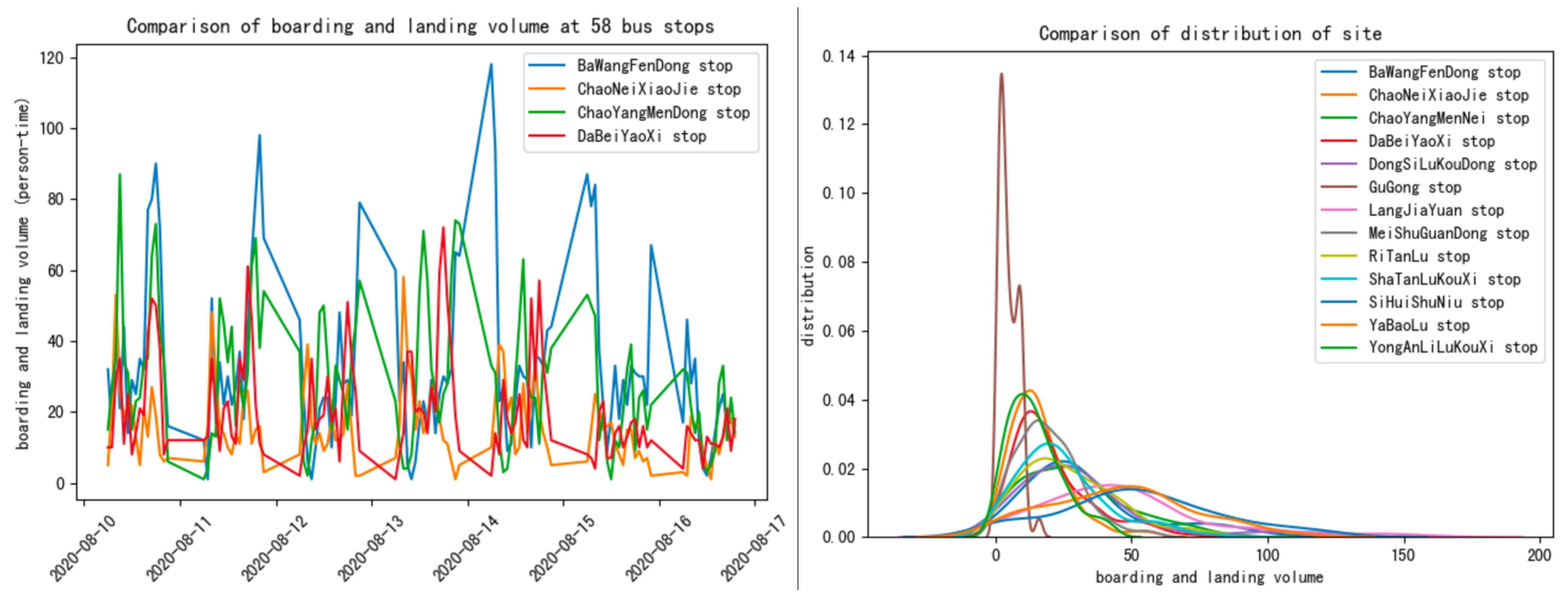
Figure 12 shows the trend and distribution of passenger flow indicators for seven bus routes. Figure 13 and Table 5 show the trend and distribution of passenger flow and stations on Route 58, The colors of the lines in Figure 12 and Figure 13 represent different bus routes and stops:

Figure 12. Trends and distribution of passenger traffic indicators (bus line).

Figure 13. Trends and distribution of passenger traffic indicators (bus stop).

Table 5. Beijing bus No.58’stops.

Site Serial Number	Stop Name	Site Serial Number	Stop Name
1	Sihui Hub Station	8	Chaoyangmennei Station
2	Bawangfen West Station	9	Chaonei Xiaojie Station
3	Langjiayuan Station	10	Dongsikou East Station
4	Dabeiyao West Station	11	Art Museum East Station
5	Yong’anli Intersection West Station	12	Beach Crossing West Station
6	Ritan Road Station	13	Palace Museum Station
7	Yabao Road Station

(3)

Data for bus network resilience analysis

The data used for the analysis of network resilience includes three datasets: “Bus Route Data,” “Bus Stop Data,” and “Bus Card Swiping Data.” In the context of studying unexpected events, the data covers a time range from 10 to 16 August 2020, spanning one week, with data collected at an hourly granularity. The unexpected event in this case is heavy rainfall on August 12. Based on the available data, this analysis selected 152 bus routes and 1547 bus stops. Prior to using the data, it is necessary to check and process redundant data, missing values, outliers, and other data issues. The necessary data filtering conditions are outlined in Table 6.

Table 6. Data filtering condition.

Condition	Value
date	10–16 August 2020
Bus line	152 bus routes
Bus stop	1547 bus stops
Bus type	Regular
Operation time	00:00–23:00
Time granularity	1 h
Running direction	Ascending, descending, ascending and descending

(4)

The handling of redundant, abnormal, and missing data.

As the basic data of bus routes and bus stops can be regarded as ordinary descriptive files, there are no significant data quality issues such as redundant data, missing values, and anomalies, making them directly usable. Therefore, the only task in the bus route data and bus stop data is to delete data fields that are irrelevant to passenger flow. By linking them through the “line code” field, they are combined into a dataset for bus routes and stops to match the IC card swipe data.

The daily IC card swipe dataset contains millions of swipe records, some of which may contain abnormal data, requiring data cleaning. The data cleaning process for the IC card swipe data in this instance mainly includes the following steps:

• Remove duplicate records: The IC card swipe dataset may have redundant and duplicate data, which needs to be removed first.
• Remove irrelevant data: Irrelevant data refers to data that does not affect the analysis of bus passenger flow, such as the creation time of a record, which can be directly deleted.
• Remove records without corresponding line codes: In the IC card swipe dataset, there are a small number of swipe records with large station indices that are not within the specified station range and must be removed.
• Remove records in “MARKSTATION” and “TRADESTATION” that do not belong to line station indices (different directions have different station indices): “MARKSTATION” and “TRADESTATION” represent boarding and alighting stations, respectively.
• Remove data where “TRADESTATION” is less than or equal to “MARKSTATION”: If the card swiping is not performed correctly, the starting and ending stations may record the same information. In such cases, abnormal data must be removed.
• Remove data in “MARKSTATION” and “TRADESTATION” that are not within the day (00:00–24:00): For IC card swipe data, two situations can lead to data quality issues. One is when passengers make card swipes incorrectly. Some passengers may forget to swipe or swipe again when getting off, so complete data will only be recorded when they swipe the card on their next trip. Therefore, the swipe records may contain boarding and alighting data that do not belong to the current day. The other situation is incomplete records during data transmission. To facilitate calculations, this paper removes swipe records that do not belong to the current day.

4.2. Experimental Process and Result

(1)

Key indicator screening

First, calculate the weights of the indicators for each of the two routes: entropy weight $w_j{}^{\left(1\right)}$ and CRITIC weight $w_j{}^{\left(2\right)}$. The results are shown in Table 7.

Table 7. Weight calculation results.

Line 1
Indicator Name	Entropy Weight Parameter			CRITIC Parameters
	${\mathit{e}}_{\mathit{j}}$	${\mathit{d}}_{\mathit{j}}$	${\mathit{w}}_{\mathit{j}}{}^{\left(1\right)}$	${\mathit{S}}_{\mathit{j}}$	${\mathit{R}}_{\mathit{j}}$	${\overline{\mathit{x}}}_{\mathit{j}}$	${\mathit{w}}_{\mathit{j}}{}^{\left(2\right)}$
Bunching (E2)	0.9476	0.0524	13.40%	22.572	11.111	250.803	1.78%
Big interval (E3)	0.9915	0.0085	2.17%	1.591	11.249	17.896	0.13%
Punctuality rate (D1)	0.998	0.002	0.50%	10.213	10.481	107.05	0.76%
Actual departure interval (A1)	0.9893	0.0107	2.75%	2.505	12.16	30.459	0.22%
Actual arrival interval (A2)	0.9892	0.0108	2.76%	2.356	11.095	26.136	0.19%
Card swiping passenger volume (B1)	0.9535	0.0465	11.89%	932.173	10.087	9402.615	66.64%
On schedule departure rate (C1)	0.9984	0.0016	0.40%	0.092	11.551	1.057	0.01%
load factor (B3)	0.9263	0.0737	18.88%	0.239	10.941	2.62	0.02%
Landing volume (B2)	0.9516	0.0484	12.38%	407.536	10.013	4080.534	28.92%
Number of online operating vehicles (C2)	0.9822	0.0178	4.56%	3.75	11.361	42.603	0.30%
Bus single-trip time (E1)	0.976	0.024	6.14%	0.299	11.772	3.521	0.02%
OD passenger flow (B4)	0.9056	0.0944	24.16%	12.809	11.333	145.154	1.03%
Line 139
Indicator Name	$e_j$	$d_j$	$w_j{}^{\left(1\right)}$	$S_j$	$R_j$	${\overline{x}}_j$	$w_j{}^{\left(2\right)}$
Bunching (E2)	0.9353	0.0647	13.70%	3.338	11.025	36.797	2.29%
Big interval (E3)	0.9833	0.0167	3.53%	1.133	12.038	13.637	0.85%
Punctuality rate (D1)	0.9968	0.0032	0.67%	9.712	10.13	98.384	6.13%
Actual departure interval (A1)	0.9899	0.0101	2.14%	2.387	10.976	26.2	1.63%
Actual arrival interval (A2)	0.9899	0.0101	2.15%	2.225	10.213	22.724	1.42%
Card swiping passenger volume (B1)	0.9164	0.0836	17.70%	97.702	9.83	960.423	59.84%
On schedule departure rate (C1)	0.998	0.002	0.43%	0.101	10.843	1.091	0.07%
Load factor (B3)	0.9471	0.0529	11.21%	0.136	10.39	1.417	0.09%
Landing volume (B2)	0.9115	0.0885	18.74%	43.358	9.669	419.244	26.12%
Number of online operating vehicles (C2)	0.9906	0.0094	2.00%	1.071	9.789	10.48	0.65%
Bus single-trip time (E1)	0.9023	0.0977	20.69%	0.353	11.084	3.911	0.24%
OD passenger flow (B4)	0.9667	0.0333	7.05%	0.958	11.037	10.574	0.66%

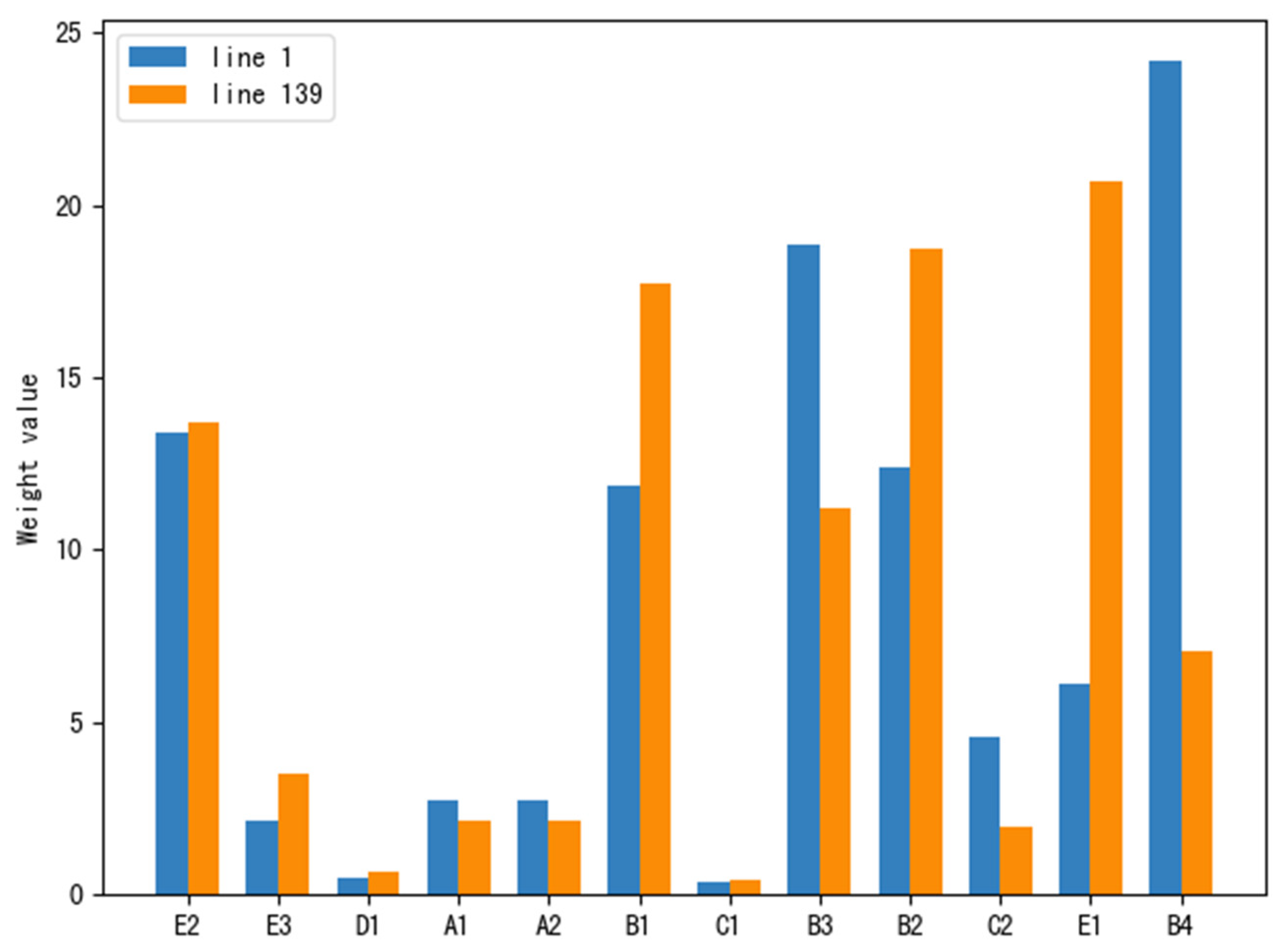
From Table 7, it can be observed that the CRITIC method adequately reflects the strength of the indicators’ comparisons and correlations. The boarding and alighting volume and the card-swiping passenger volume show significant variations, indicating that these two indicators can reflect more information. On the other hand, the entropy weight method indirectly reflects the importance of indicators based on their degree of dispersion. For indicators with larger variations in the CRITIC method, their information entropy is relatively smaller, which confirms that they contain more information. The weights obtained from the two methods are compared in Figure 14 and Figure 15.

Figure 14. Entropy weight method weight comparison (x-axis: indicator code).

Figure 15. Comparison of critic weights (x-axis: indicator code).

From the figures, it can be observed that in the entropy weight method, the weights of indicators such as boarding and alighting volume, occupancy rate, card-swiping passenger volume, and occurrence of bus bunching are all above 10%, significantly higher than the weights of other indicators. Additionally, Route 1’s OD passenger flow and Route 139’s card-swiping passenger volume also have relatively high weights. In the CRITIC weights, the weights of card-swiping passenger volume and boarding and alighting volume both exceed 20%, leading significantly compared to other indicators. Based on the obtained weights $w_j{}^{\left(1\right)}$ and $w_j{}^{\left(2\right)}$, the total weights $w_j$ can be calculated. The results are shown in Table 8.

Table 8. Weight ranking results.

Indicator Name	$\mathbf{Line}1\prime \mathbf{s}{\mathit{w}}_{\mathit{j}}$	Ranking	$\mathbf{Line}139\prime \mathbf{s}{\mathit{w}}_{\mathit{j}}$	Ranking
Bunching (E2)	7.59	5	7.995	4
Big interval (E3)	1.15	10	2.19	8
Punctuality rate (D1)	0.63	11	3.4	7
Actual departure interval (A1)	1.485	8	1.885	9
Actual arrival interval (A2)	1.475	9	1.785	10
Card swiping passenger volume (B1)	39.265	1	38.77	1
On schedule departure rate (C1)	0.205	12	0.25	12
Load factor (B3)	9.45	4	5.65	5
Landing volume (B2)	20.65	2	22.43	2
Number of online operating vehicles (C2)	2.43	7	1.325	11
Bus single-trip time (E1)	3.08	6	10.465	3
OD passenger flow (B4)	12.595	3	3.855	6

Comparing the total weight rankings of the two routes, it can be observed that the total weights of card-swiping passenger volume and boarding and alighting volume are significantly higher than other indicators. The total weights of card-swiping passenger volume are 39.265 and 38.77, while the total weights of boarding and alighting volume are 20.65 and 22.43, respectively. Therefore, we can conclude that according to the CRITIC–entropy weight evaluation model, card-swiping passenger volume is a key indicator in the evaluation system for monitoring the operational status of the bus network and can be used to calculate the bus network’s resilience.

(2)

Bus route resilience analysis

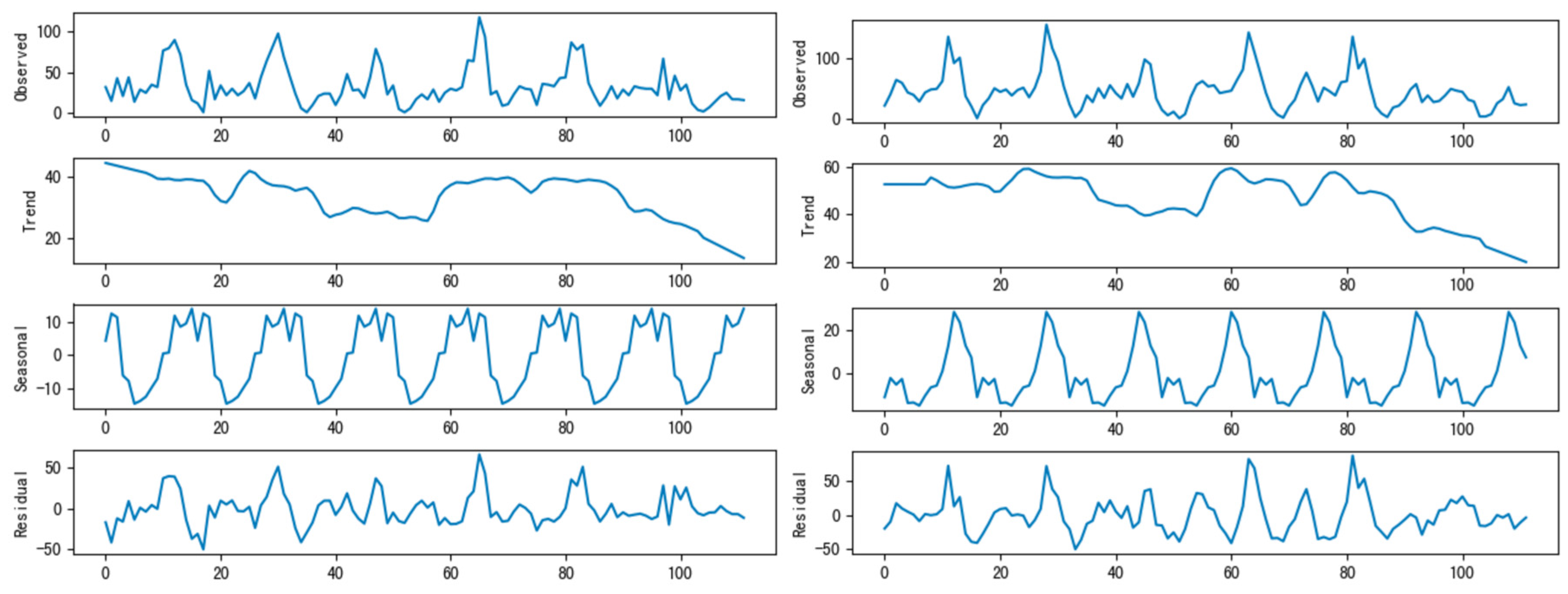
In this example analysis, data processing and calculations are performed using Python and related packages. First, the data of each indicator is smoothed using the STL (seasonal and trend decomposition using Loess) time series decomposition method for indicators with significant seasonality and periodicity, such as card-swiping passenger volume and boarding and alighting volume. STL is a versatile and robust method that stands for “Seasonal and Trend decomposition using Loess,” where Loess refers to a robust regression algorithm. One of the advantages of this algorithm is that the seasonal component can vary over time with controllable changing rates. STL provides a separate multiplicative trend for the seasonal part, which allows for increasing amplitudes when using an additive model. Additionally, STL is robust to outliers, meaning that outliers do not significantly affect the seasonal and trend components. Figure 16 shows the trend and seasonal variations of card-swiping passenger volume for some routes (Route 1, Route 139, Route 101, and Route 116) after STL decomposition.

Figure 16. Trend of line passenger flow index after STL decomposition (x-axis: serialized time).

Figure 17 represents the trend and seasonal variations of passenger boarding and alighting at the Bawangfen East stop and Langjiayuan stop after applying the STL decomposition method.

Figure 17. Trend of stop passenger flow index after STL decomposition (x-axis: serialized time).

By observing the trend of each indicator after applying STL decomposition, it can be noticed that there is a significant decrease followed by an increase between time scales 25 to 65, which is influenced by the rainfall from August 12th to 13th. This pattern represents a complete resilience cycle. The declining trend after time scale 80 is mainly due to the decrease in commuting demand from citizens during weekends. This analysis focuses mainly on the variations within the resilience cycle.

The next step is to determine the time when each indicator reaches a steady state and the corresponding steady-state value within the resilience cycle. This involves extracting a subset of data for each indicator within the $\left[t_L,t_E\right]$ timeframe. The augmented Dickey–Fuller (ADF) test is then applied to this subset using an autoregressive process with drift and trend terms. If the p-value of the ADF test for the period $\left[t_{test},t_E\right](t_{test}>t_L)$ is less than 0.05, it indicates that the subset of data is stationary, and the steady-state time is defined as $t_{SS}=t_{test}$ and the steady-state value as $y_S=y\left(t_{test}\right)$.

After obtaining $t_{SS}$ and $y_S$ for each indicator, the resilience factors $\theta$, $\rho$, $\lambda$, $\sigma$, $\tau$, and the overall resilience $R_l$ are calculated. The volatility coefficient $\sigma$ is computed using the raw indicator data, denoted as $y_{raw}\left(t\right)$, and the smoothed data obtained through STL decomposition, denoted as $y_s\left(t\right)$.

The resilience factors and overall resilience for the seven analyzed routes, in this case, study are shown in Table 9.

Table 9. Resilience factors and total resilience of 7 lines.

Line	$\mathit{\theta }$	$\mathit{\lambda }$	$\mathit{\rho }$	$\mathit{\tau }$	$\mathit{\sigma }$	${\mathit{R}}_{\mathit{l}}$
1	0.6127	0.0792	0.8913	0.6238	0.3261	0.3952
139	0.6791	0.4331	0.7896	0.7139	0.3968	0.5057
101	0.5292	0.0852	1.1572	0.7029	0.4519	0.5216
116	0.6154	0.0841	1.1229	0.7316	0.3742	0.5083
27	0.4687	0.1127	0.8446	0.638	0.4929	0.3507
40	0.5983	0.1481	1.1795	0.7179	0.3484	0.5547
60	0.4894	0.0936	0.7022	0.4313	0.4204	0.3143

The resilience factors and overall resilience for the thirteen analyzed stations, in this case, study are shown in Table 10.

Table 10. Resilience factors and total resilience of 13 stops.

Bus Stop	$\mathit{\theta }$	$\mathit{\lambda }$	$\mathit{\rho }$	$\mathit{\tau }$	$\mathit{\sigma }$	${\mathit{R}}_{\mathit{l}}$
Sihui Hub Station	0.5125	0.2189	0.8101	0.5552	0.3911	0.3752
Bawangfen West Station	0.4344	0.6237	0.9912	0.6792	0.4463	0.5178
Langjiayuan Station	0.3124	0.2935	0.8646	0.7919	0.3048	0.1953
Dabeiyao West Station	0.5213	0.6892	0.6774	0.5481	0.4685	0.4063
Yong’anli Intersection West Station	0.7525	0.3487	0.9344	0.5598	0.2839	0.6474
Ritan Road Station	0.4687	0.65	0.8789	0.7931	0.2486	0.3915
Yabao Road Station	0.5173	0.4885	0.6564	0.6884	0.3299	0.2985
Chaoyangmennei Station	0.458	0.5502	1.0466	0.4297	0.4176	0.6281
Chaonei Xiaojie Station	0.6182	0.8047	1.1535	0.7485	0.4337	0.9516
Dongsikou East Station	0.251	0.2625	1.3992	0.6247	0.3671	0.3666
Art Museum East Station	0.3462	0.353	0.8743	0.6163	0.2468	0.2490
Beach Crossing West Station	0.6369	0.4892	0.891	0.2988	0.3981	0.7217
Palace Museum Station	0.3748	0.2293	0.8367	0.7438	0.2956	0.2162

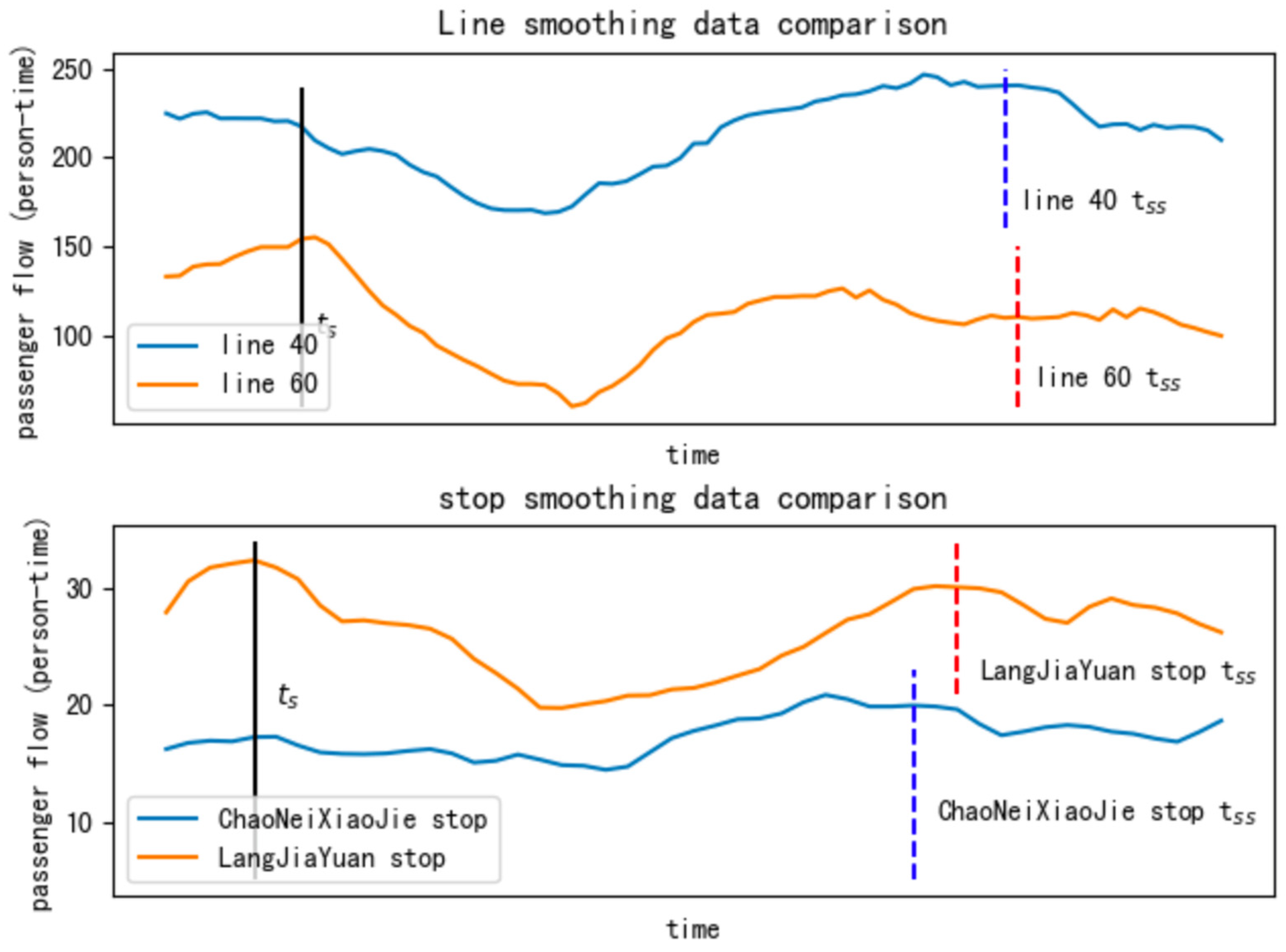
From the observation of Figure 18 and the comparison of experimental results, it can be concluded that among the seven analyzed routes, Route 40 exhibits the highest resilience. This is mainly attributed to its higher values of the absorption factor $\lambda$ and the recovery factor $\rho$. These factors indicate that Route 40 has better absorption and recovery capabilities during the resilience cycle, resulting in an overall enhancement of resilience. On the other hand, Route 60 has the lowest resilience value, primarily due to its weaker absorption capability during the resilience cycle and higher sensitivity of indicators to disruptive events.

Figure 18. Smooth data comparison.

Among the thirteen analyzed stations, the Chaoneixiaojie station demonstrates the highest resilience value. This is also because it possesses higher absorption and recovery capabilities, as indicated by $\rho >1$, indicating that the indicator values exceed the initial values when reaching the steady state. By comparing the smoothed data in the plots, it is evident that the trend of Route 40 is significantly less affected by the disruptive event within the $\left[t_S,t_{SS}\right]$ interval compared to Route 60. The comparison between the two stations further emphasizes this point, as the passenger volume at Chaoneixiaojie station during the resilience cycle is minimally affected by the disruptive event, showcasing its superior recovery and absorption capabilities compared to Langjiayuan station.

Based on this case analysis, it can be concluded that the proposed resilience analysis model based on resilience cycles effectively and accurately assesses the resilience of bus routes affected by disruptive events. The resilience values calculated for the bus routes in this section will serve as inputs for the overall resilience analysis of the bus network. These values will be used to compute the overall resilience of the bus network.

(3)

Bus network resilience analysis

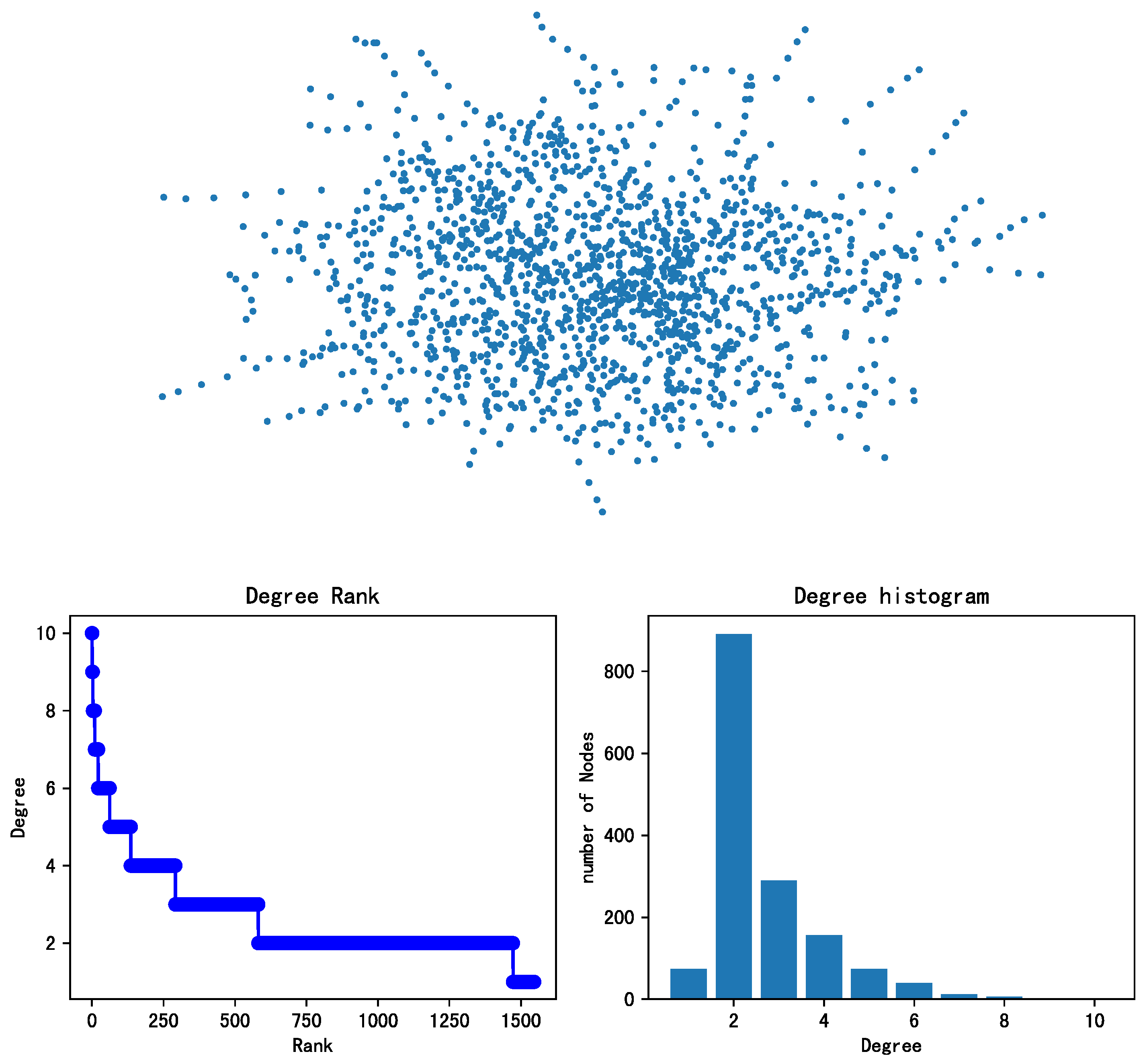
First, the data of 152 bus routes and 1547 bus stations are abstracted into a topology graph using the NetworkX tool package in Python. The result is shown in Figure 19.

Figure 19. Topological structure and degree distribution of public transit network.

From the degree distribution in Figure 19, it can be observed that the bus network exhibits a scale-free property, where the degree values follow a power law distribution. This means that a small number of nodes have relatively high degrees, while the majority of nodes have lower degrees. This observation aligns with the natural distribution of bus network stations, as there are typically only a few major transportation hubs. Such networks are often referred to as heterogeneous networks. The partial statistical characteristics of the bus network in this study are shown in Table 11.

Table 11. Public transit network statistics.

Statistical Characteristics	Value
Network diameter	81
Network average distance	17.1582
Network local efficiency	0.0830
Global network efficiency	0.0692
Network average clustering coefficient	0.0776
Global clustering coefficient of the network	0.1186

From the statistical features, it can be observed that the network has relatively low local and global efficiency, indicating that the network has limited global transmission capacity and resilience against small-scale failures. The clustering coefficient is a measure of the degree of clustering among nodes in a network, calculated as the ratio of the number of edges between a node’s neighbors to the maximum possible number of edges between these neighbors. The network’s average clustering coefficient is obtained by averaging the clustering coefficients of all nodes in the network, reflecting the network’s clustering tendency. From the average clustering coefficient of the network, it can be inferred that the network has a relatively low level of clustering. Figure 20 presents four centrality measures for the public transportation network consisting of 152 bus routes. It can be observed that the node closeness centrality and edge betweenness centrality are relatively concentrated, indicating that centrality measures can effectively capture the network’s importance.

Figure 20. Four centrality indexes of public transit network topology (x-axis: index value, y-axis: number of indexes.).

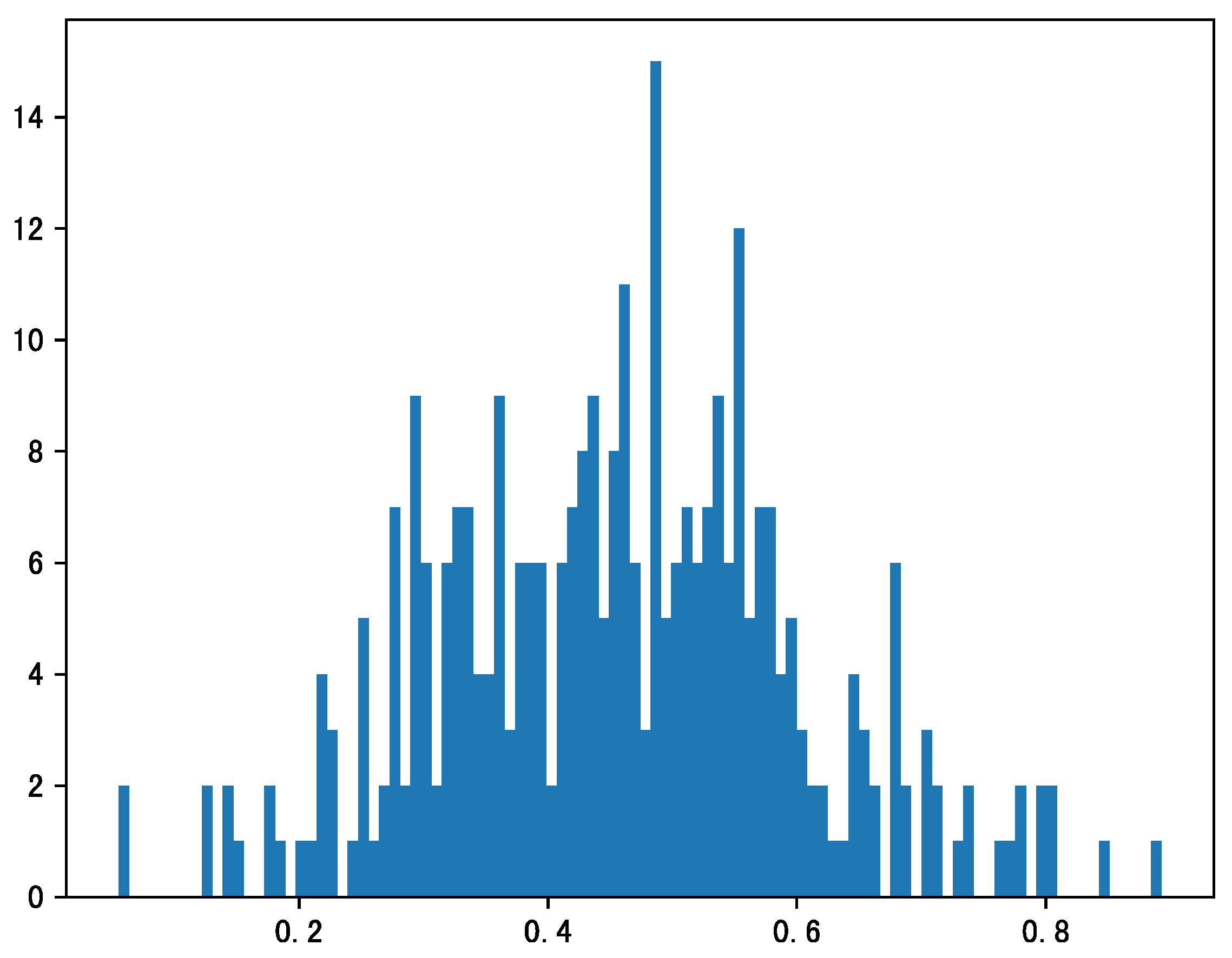
Next, the resilience values of the 152 bus routes are calculated based on the bus card swipe passenger flow data and normalized. The normalized weights of the routes are shown in Figure 21.

Figure 21. Bus network route weight distribution (x-axis: resilience value, y-axis: number of routes.).

Then, the weights of the routes are input into the network topology to form a weighted scale-free network. The average resilience values of the nodes and edges are calculated separately, and the arithmetic mean of these values is obtained as $R_{total}$. Here, the weighted network resilience value $R_{total}$ is compared with the resilience value R’ of the unweighted network. $R\prime$ is calculated by taking the average of the normalized node closeness centrality and the normalized edge betweenness centrality. The difference between the two is that $R_{total}$ takes into account the resilience weights of the bus routes, while R’ only considers the centrality of nodes and edges.

The resilience values of the network are calculated separately for comparison, and the results are shown in Table 12.

Table 12. Bus network resilience calculation results.

${\mathit{R}}_{\mathit{t}\mathit{o}\mathit{t}\mathit{a}\mathit{l}}$	$\mathit{R}’$
0.3716	0.4501

The top five nodes and edges with the highest resilience values in the calculation of $R_{total}$ are shown in Table 13.

Table 13. The top five nodes and lines by resilience value.

Stop Name	${\mathit{C}}_{\mathit{C}}{}^{’}\left({\mathit{v}}_{\mathit{i}}\right)$	Section	${\mathit{C}}_{\mathit{B}}{}^{’}\left({\mathit{e}}_{\mathit{l}}\right)$
Xibahe Station	0.07737	Laiguangying Intersection West Station–Dongzhimen Hub Station	0.14812
Dongzhimen Hub Station	0.07713	Laiguangying Intersection West Station–Xibahe Station	0.14753
Laiguangying Intersection West Station	0.07692	Xima Community Station–Taiping Street Station	0.14407
Yuquan Yingqiao North Station	0.07633	Taiping Street Station–Zengguang Road East Station	0.14239
Beach Crossing West Station	0.07611	Yuanda Road Station–Jiaojiafen Intersection East Station	0.13564

The five nodes and five edges in Table 13 have higher resilience, indicating that they are less affected by unexpected events. There are 49 bus routes passing through these 5 nodes, and it can be observed that these nodes are located near interchange hubs such as overpasses. Moreover, the bus routes passing through these edges mostly cover other important transportation hubs. The experimental results reflect the effectiveness of the resilience calculation model proposed in this study.

5. Conclusions and Outlook

5.1. Conclusions

To accurately quantify the resilience of the bus network, this paper constructs a research framework for bus network resilience from the perspectives of spatio-temporal dynamics and structural statics of the bus network. The framework can be divided into three parts:

• A key indicator selection method based on CRITIC–entropy weighting is proposed. Based on 12 specific indicator items extracted from the monitoring indicators of bus network operations, the weights of each indicator are analyzed, calculated, and ranked from the aspects of entropy value, information redundancy, variability, and conflict. The key indicator that can best reflect the changes in bus route status is determined to be the card-swiping passenger flow.
• Based on the resilience cycle theory, a resilience analysis model for route resilience is built by considering the resilience cycles of card-swiping passenger flows for each route and station under the impact of unexpected events. After verifying the scientificity of the model, resilience is calculated, analyzed, and compared using data from seven bus routes and 17 stations of Route 58.
• Based on complex network theory, a resilience analysis model for the bus network is constructed. The resilience values of bus routes are used as the weights of network edges, and the bus routes are treated as edges while the bus stations are treated as nodes to construct an undirected weighted complex network of the bus network. By calculating the node closeness centrality and edge betweenness centrality indicators in the complex network, weighted by edge weights, a quantitative model for quantifying bus network resilience is established. The proposed model is applied to a case study involving 152 bus routes and 1547 bus stations, calculating the resilience of the bus network during a period of heavy rain from 10 to 16 August 2020.

The research presented in this paper introduces a comprehensive framework for analyzing the resilience of bus networks in the context of unexpected events. This framework provides research methods and a foundation for the analysis and optimization of bus network resilience. Additionally, the research findings of this paper can be utilized by bus network operators and planning departments to evaluate the strengths and weaknesses of bus networks, as well as provide decision-making guidance for adjusting and optimizing bus routes and stations.

5.2. Outlook

This study is based on real multi-source data and utilizes various mature theories and algorithms to model, analyze, and validate the resilience of bus networks. It has obtained research results of high theoretical and practical significance. However, there are areas for improvement and further development in the study.

The research findings of this study are oriented toward bus network managers and operators, and the data used are collected from the bus operation process. In the future, if passenger data can be integrated (such as passenger location and passenger origin–destination pairs), conducting bus network resilience analysis from the perspective of passengers will enhance the generality and versatility of the research outcomes.

Although the study attempted to incorporate emergency events other than adverse weather conditions for analyzing the resilience of bus networks, it is regrettable that due to the limited time span of the available bus data, only a few emergency events related to adverse weather conditions could be matched with the multi-source bus data for that period. In future research, if it is possible to acquire multi-source bus data that match various types of emergency events, it would enable the validation of the proposed bus network resilience analysis model in different emergency scenarios. This would allow for a comparative analysis of the resilience of bus networks under different types of emergency events, which would yield more meaningful research results.

The real bus data used in this study are sourced from Beijing Public Transport Group and Beijing Municipal Traffic Operation Monitoring and Dispatching Center. Therefore, all the case analyses are based on the bus network in Beijing. While Beijing’s bus network ranks among the top five in terms of network density and scale in the national bus system, it is essential to consider the uniqueness of bus networks in different cities. In future research, if it is possible to obtain multi-source integrated data for bus networks in different cities, it would optimize this study from the perspectives of universality and applicability. Additionally, it would allow for a comparative analysis of the different responses of bus networks in different cities to emergency events, thereby making the research findings more significant in terms of theory and practicality.

References

1. Yunes, M.A.M. Psicologia positiva e resiliência: O foco no indivíduo e na família. Psicol. Estud. 2003, 8, 75–84. [Google Scholar] [CrossRef]
2. Nagatsu, M.; Davis, T.; DesRoches, C.T.; Koskinen, I.; MacLeod, M.; Stojanovic, M.; Thoren, H. Philosophy of science for sustainability science. Sustain. Sci. 2020, 15, 1807–1817. [Google Scholar] [CrossRef]
3. Holling, C.S. Surprise for science, resilience for ecosystems, and incentives for people. Ecol. Appl. 1996, 6, 733–735. [Google Scholar] [CrossRef]
4. Walker, B.; Carpenter, S.; Anderies, J.; Abel, N.; Cumming, G.; Janssen, M.; Lebel, L.; Norberg, J.; Peterson, G.D.; Pritchard, R. Resilience management in social-ecological systems: A working hypothesis for a participatory approach. Conserv. Ecol. 2002, 6, 14. [Google Scholar] [CrossRef]
5. Zhou, Y.; Wang, J.; Yang, H. Resilience of Transportation Systems: Concepts and Comprehensive Review. IEEE Trans. Intell. Transp. Syst. 2019, 20, 4262–4276. [Google Scholar] [CrossRef]
6. Li, Y.; Zhao, L. Analyzing Deformation of Supply Chain Resilient System Based on Cell Resilience Model. In Lecture Notes in Computer Science, Proceedings of the Life System Modeling and Intelligent Computing, Pt I, Wuxi, China, 17–20 September 2010; Li, K., Fei, M.R., Jia, L., Irwin, G.W., Eds.; Springer: Berlin, Germany, 2010; Volume 6328, pp. 26–35. [Google Scholar]
7. Adams, G.; Bell, C. The quest for resilience. Harv. Bus. Rev. 2004, 82, 116. [Google Scholar]
8. Patriarca, R.; Di Gravio, G.; Costantino, F.; Tronci, M.; Severoni, A.; Vernile, A.; Bilotta, F. A paradigm shift to enhance patient safety in healthcare, a resilience engineering approach: Scoping review of available evidence. Int. J. Healthc. Technol. Manag. 2017, 16, 319–343. [Google Scholar] [CrossRef]
9. Mayar, K.; Carmichael, D.G.; Shen, X. Resilience and Systems—A Review. Sustainability 2022, 14, 8327. [Google Scholar] [CrossRef]
10. Bhamra, R.; Dani, S.; Burnard, K. Resilience: The concept, a literature review and future directions. Int. J. Prod. Res. 2011, 49, 5375–5393. [Google Scholar] [CrossRef]
11. Anderies, J.M.; Walker, B.H.; Kinzig, A.P. Fifteen weddings and a funeral: Case studies and resilience-based management. Ecol. Soc. 2006, 11, 21. [Google Scholar] [CrossRef]
12. Carpenter, S.; Walker, B.; Anderies, J.M.; Abel, N. From metaphor to measurement: Resilience of what to what? Ecosystems 2001, 4, 765–781. [Google Scholar] [CrossRef]
13. Miller, F.; Bowen, K. Questioning the assumptions: The role of vulnerability assessments in climate change adaptation. Impact Assess. Proj. Apprais. 2013, 31, 190–197. [Google Scholar] [CrossRef]
14. Eriksen, S.; Schipper, E.L.F.; Scoville-Simonds, M.; Vincent, K.; Adam, H.N.; Brooks, N.; Harding, B.; Khatri, D.; Lenaerts, L.; Livermanm, D.; et al. Adaptation interventions and their effect on vulnerability in developing countries: Help, hindrance or irrelevance? World Dev. 2021, 141, 105383. [Google Scholar] [CrossRef]
15. Younus, M.A.F.; Kabir, M.A. Climate Change Vulnerability Assessment and Adaptation of Bangladesh: Mechanisms, Notions and Solutions. Sustainability 2018, 10, 4286. [Google Scholar] [CrossRef]
16. Joakim, E.P.; Mortsch, L.; Oulahen, G. Using vulnerability and resilience concepts to advance climate change adaptation. Environ. Hazards 2015, 14, 137–155. [Google Scholar] [CrossRef]
17. Pamungkas, A.; Bekessy, S.A.; Lane, R. Vulnerability Modelling to Improve Assessment Process on Community Vulnerability. In Proceedings of the Resilient Cities: Beyond Mitigation, Preparedness, Response, and Recovery (Cities 2013 International Seminar); Pamungkas, A., Das, A., Supriharjo, R., Santoso, E.B., Sagala, S., Eds.; Elsevier Science Bv: Amsterdam, The Netherlands, 2014; Volume 135, pp. 159–166. [Google Scholar]
18. Simonovic, S.P.; Arunkumar, R. Comparison of static and dynamic resilience for a multipurpose reservoir operation. Water Resour. Res. 2016, 52, 8630–8649. [Google Scholar] [CrossRef]
19. Petersen, B.; Aslan, C.; Stuart, D.; Beier, P. Incorporating Social and Ecological Adaptive Capacity into Vulnerability Assessments and Management Decisions for Biodiversity Conservation. Bioscience 2018, 68, 371–380. [Google Scholar] [CrossRef]
20. Whitney, C.K.; Bennett, N.J.; Ban, N.C.; Allison, E.H.; Armitage, D.; Blythe, J.L.; Burt, J.M.; Cheung, W.; Finkbeiner, E.M.; Kaplan-Hallam, M.; et al. Adaptive capacity: From assessment to action in coastal social-ecological systems. Ecol. Soc. 2017, 22, 22. [Google Scholar] [CrossRef]
21. Chen, B.N. Research on Assessment Method of Urban Water System’s Adaptability to Heavy Rainfall; Beijing University of Civil Engineering and Architecture: Beijing, China, 2019. [Google Scholar]
22. Erdiaw-Kwasie, M.O.; Abunyewah, M.; Yamoah, O. “After the disaster comes destination thoughts”: A review and conceptualization of consolidative disaster adaptive capacity model. Int. J. Disaster Risk Reduct. 2019, 35, 101098. [Google Scholar] [CrossRef]
23. Elrick-Barr, C.E.; Plummer, R.; Smith, T.F. Third-generation adaptive capacity assessment for climate-resilient development. Clim. Dev. 2021, 15, 518–521. [Google Scholar] [CrossRef]
24. Lu, Y.; Zhai, G.; Zhou, S.; Shi, Y. Risk reduction through urban spatial resilience: A theoretical framework. Hum. Ecol. Risk Assess. 2021, 27, 921–937. [Google Scholar] [CrossRef]
25. Fiksel, J. Designing resilient, sustainable systems. Environ. Sci. Technol. 2003, 37, 5330–5339. [Google Scholar] [CrossRef] [PubMed]
26. Zhen, Z.; Wang, F.B. Dynamic Evolution of Resilience in the Global Value Chain System under Adverse Events Impact: A Longitudinal Study Based on Embedded Multiple Cases. China Ind. Econ. 2022, 10, 174–192. [Google Scholar] [CrossRef]
27. Cutter, S.L.; Ahearn, J.A.; Amadei, B.; Crawford, P.; Eide, E.A.; Galloway, G.E.; Goodchild, M.F.; Kunreuther, H.C.; Li-Vollmer, M.; Schoch-Spana, M.; et al. Disaster Resilience: A National Imperative. Environment 2013, 55, 25–29. [Google Scholar] [CrossRef]
28. Xu, J. Governance of Urban Public Transportation Resilience under Public Health Emergencies. Urban Transp. 2020, 18, 98–101+9. [Google Scholar] [CrossRef]
29. Zhu, J.; Zhang, L.; Ren, Z. A Conceptual Framework for Understanding the Relationships between Transportation Infrastructure and Human Resilience. In Proceedings of the Construction Research Congress 2020: Infrastructure Systems and Sustainability; ElAsmar, M., Tang, P., Grau, D., Eds.; Amer Soc Civil Engineers: New York, NY, USA, 2020; pp. 361–369. [Google Scholar]
30. Yang, C.; Tang, P.; Hao, X.; Li, X. Resilient Transportation Construction Practice and Enlightenment. Compr. Transpor-Tation 2021, 43, 134–138. [Google Scholar]
31. Xu, X.; Chen, A.; Xu, G.; Yang, C.; Lam, W.H.K. Enhancing network resilience by adding redundancy to road networks. Transp. Res. Part E Logist. Transp. Rev. 2021, 154, 102448. [Google Scholar] [CrossRef]
32. Liu, J.; Zhang, L.; Shi, Z.; Wang, Y. Review of Resilience Research in Transportation Systems. Sci. Technol. Ind. 2020, 20, 47–52. [Google Scholar]
33. Murray-Tuite, P.M. A comparison of transportation network resilience under simulated system optimum and user equilibrium conditions. In Proceedings of the 2006 Winter Simulation Conference, Monterey, CA, USA, 3–6 December 2006; IEEE: New York, NY, USA, 2006; Volume 1–5, pp. 1398–1405. [Google Scholar]
34. Ji, T.; Yao, Y.; Dou, Y.; Deng, S.; Yu, S.; Zhu, Y.; Liao, H. The Impact of Climate Change on Urban Transportation Resilience to Compound Extreme Events. Sustainability 2022, 14, 3880. [Google Scholar] [CrossRef]
35. Twumasi-Boakye, R.; Sobanjo, J.O. Resilience of Regional Transportation Networks Subjected to Hazard-Induced Bridge Damages. J. Transp. Eng. Pt A-Syst. 2018, 144, 04018062. [Google Scholar] [CrossRef]
36. Ilbeigi, M. Statistical process control for analyzing resilience of transportation networks. Int. J. Disaster Risk Reduct. 2019, 33, 155–161. [Google Scholar] [CrossRef]
37. Argyroudis, S.A. Resilience metrics for transport networks: A review and practical examples for bridges. Proc. Inst. Civ. Eng.-Bridge Eng. 2022, 175, 179–192. [Google Scholar] [CrossRef]
38. Zhang, X. Safety and Resilience Evaluation of Urban Rail Transit Operation Systems. Master’s Thesis, Shijiazhuang Tiedao University, Shaoxing, China, 2022. [Google Scholar]
39. Janic, M. Analysis and modelling of airport resilience, robustness, and vulnerability: Impact of COVID-19 pandemic disease. Aeronaut. J. 2022, 126, 1924–1953. [Google Scholar] [CrossRef]
40. He, Z.; Navneet, K.; van Dam, W.; Van Mieghem, P. Robustness assessment of multimodal freight transport networks. Reliab. Eng. Syst. Saf. 2021, 207, 107315. [Google Scholar] [CrossRef]
41. Besinovic, N. Resilience in railway transport systems: A literature review and research agenda. Transp. Rev. 2020, 40, 457–478. [Google Scholar] [CrossRef]
42. Faturechi, R.; Miller-Hooks, E. Measuring the Performance of Transportation Infrastructure Systems in Disasters: A Comprehensive Review. J. Infrastruct. Syst. 2015, 21, 04014025. [Google Scholar] [CrossRef]
43. Liu, C.; Fan, Y.; Ordonez, F. A two-stage stochastic programming model for transportation network protection. Comput. Oper. Res. 2009, 36, 1582–1590. [Google Scholar] [CrossRef]
44. Wu, F.; Schonfeld, P.M.; Ayyub, B.; Kim, M. Topological Approach for Optimizing Railroad Freight Network Restoration after Disruptions. Transp. Res. Rec. 2022, 2676, 750–759. [Google Scholar] [CrossRef]
45. Chen, M.; Mangalathu, S.; Jeon, J.-S. Seismic reliability assessment of bridge networks considering travel time and connectivity reliabilities. Earthq. Eng. Struct. Dyn. 2022, 51, 3097–3110. [Google Scholar] [CrossRef]
46. Chopra, S.S.; Dillon, T.; Bilec, M.M.; Khanna, V. A network-based framework for assessing infrastructure resilience: A case study of the London metro system. J. R. Soc. Interface 2016, 13, 20160113. [Google Scholar] [CrossRef]
47. Dong, B.-X.; Shan, M.; Hwang, B.-G. Simulation of transportation infrastructures resilience: A comprehensive review. Environ. Sci. Pollut. Res. 2022, 29, 12965–12983. [Google Scholar] [CrossRef] [PubMed]
48. Serulle, N.U.; Heaslip, K.; Brady, B.; Louisell, W.C.; Collura, J. Resiliency of Transportation Network of Santo Domingo, Dominican Republic Case Study. Transp. Res. Rec. 2011, 2234, 22–30. [Google Scholar] [CrossRef]
49. Xu, Z.; Chopra, S.S.; Lee, H. Resilient Urban Public Transportation Infrastructure: A Comparison of Five Flow-Weighted Metro Networks in Terms of the Resilience Cycle Framework. IEEE Trans. Intell. Transp. Syst. 2022, 23, 12688–12699. [Google Scholar] [CrossRef]
50. Ma, B.; Chai, H.; Zhang, Z. Exploration of Passenger Flow Characteristics and Resilience in Urban Rail Transit during the Post-Epidemic Period. Compr. Transp. 2022, 44, 75–80. [Google Scholar]
51. Ip, W.H.; Wang, D. Resilience and Friability of Transportation Networks: Evaluation, Analysis and Optimization. IEEE Syst. J. 2011, 5, 189–198. [Google Scholar] [CrossRef]
Disclaimer/Publisher’s Note: The statements, opinions and data contained in all publications are solely those of the individual author(s) and contributor(s) and not of MDPI and/or the editor(s). MDPI and/or the editor(s) disclaim responsibility for any injury to people or property resulting from any ideas, methods, instructions or products referred to in the content.
Article Metrics
Citations
Article Access Statistics
Multiple requests from the same IP address are counted as one view.