A Robust and Secure Watermarking Approach Based on Hermite Transform and SVD-DCT

Abstract

Currently, algorithms to embed watermarks into digital images are increasing exponentially, for example in image copyright protection. However, when a watermarking algorithm is applied, the preservation of the image’s quality is of utmost importance, for example in medical images, where improper embedding of the watermark could change the patient’s diagnosis. On the other hand, in digital images distributed over the Internet, the owner of the images must also be protected. In this work, an imperceptible, robust, secure, and hybrid watermarking algorithm is presented for copyright protection. It is based on the Hermite Transform (HT) and the Discrete Cosine Transform (DCT) as a spatial–frequency representation of a grayscale image. Besides, it uses a block-based strategy and a perfectibility analysis of the best embedding regions inspired by the Human Vision System (HVS), giving the imperceptibility of the watermark, and a Singular-Value Decomposition (SVD) approach improved robustness against attacks. In addition, the proposed method can embed two watermarks, a digital binary image (LOGO) and information about the owner and the technical data of the original image in text format (MetaData). To secure both watermarks, the proposed method uses the Jigsaw Transform (JST) and the Elementary Cellular Automaton (ECA) to encrypt the image LOGO and a random sequence generator and the XOR operation to encrypt the image MetaData. On the other hand, the proposed method was tested using a public dataset of 49 grayscale images to assess the effectiveness of the watermark embedding and extraction procedures. Furthermore, the proposed watermarking algorithm was evaluated under several processing and geometric algorithms to demonstrate its robustness to the majority, intentional or unintentional, attacks, and a comparison was made with several state-of-the-art techniques. The proposed method obtained average values of PSNR = 40.2051 dB, NCC = 0.9987, SSIM = 0.9999, and MSSIM = 0.9994 for the watermarked image. In the case of the extraction of the LOGO, the proposal gave MSE = 0, PSNR ≫ 60 dB, NCC = 1, SSIM = 1, and MSSIM = 1, whereas, for the image MetaData extracted, it gave BER = 0% and $B_{error}=0$. Finally, the proposed encryption method presented a large key space ($K=1.2689\times {10}^{89}$) for the LOGO image.

1. Introduction

Currently, digital watermarking has become a way to embed information into an image and protect it from unauthorized access and manipulation. Depending on digital content such as video, image, audio, and text and the application, algorithms can be developed for authentication, material security, trademark protection, and the tracking of digital content. The objective is to insert a watermark (digital image or text) into the digital content. There are important requirements to take into account when a watermarking algorithm is designed: imperceptibility, robustness, security, capacity, and computational cost. It is difficult to have an algorithm that embraces all requirements due to robustness, which refers to the ability to withstand image distortions that may compromise the imperceptibility of the watermark. Because of that, different techniques have been developed in order to improve robustness without compromising the original content. The state-of-the-art suggests that these algorithms can be designed in the spatial, transform, or hybrid domain. Thus, the algorithms alter the marked pixels to embed the watermark in the intensity domain of the image. The advantage of this is low computational complexity; however, the image suffers visible alterations, and the algorithm does not possess robustness against geometric transformations. In the transform domain, the watermark is embedded within specific elements to ensure enhanced resilience. Furthermore, the transforms can be combined to have hybrid domain watermarking. These kinds of methods increase the performance of the watermarking technique.

Therefore, in a watermarking image method, the watermark must be robust and imperceptible or perceptible, depending on the application. In this paper, we propose a hybrid, robust, and imperceptibility watermarking approach using the Hermite Transform (HT), Singular-Value Decomposition (SVD), the Human Vision System (HVS), and the Discrete Cosine Transform (DCT) to protect digital images. As watermarks, we used a digital image LOGO and image MetaData (with information about the original image or the owner), so we inserted two different digital contents into a digital image. The Hermite transform is based on the Gaussian function derivatives, and it incorporates human visual system properties, so it allows a perfect reconstruction of the image. To have more security, the LOGO is encrypted using the Jigsaw Transform (JST) before inserting. In addition, the indexes to decrypt the LOGO are secured using the Elementary Cellular Automaton (ECA), increasing the security of the proposal. In addition, the image MetaData are secured using a random sequence generator and the XOR operation. Finally, the Hamming error correcting code was applied to the image MetaData to reduce channel distortion.

The rest of the paper is divided as follows: Section 2 presents the related work describing the image watermarking methods using the DCT and SVD techniques and other space–frequency decomposition methods similar to the HT. We describe all the elements used to design the watermark algorithm such as the public dataset, JST, SVD, HT, DCT, HVS, and Elementary Cellular Automata (ECA) in Section 3. Section 4 details the proposed watermarking algorithm for the insertion/extraction of the watermarks. In Section 5, we report the experiments and results obtained in the insertion and extraction stages of the watermarks, including the computational complexity of the algorithm. In addition, we report the robustness analysis of the proposed method against the most-common processing and geometric attacks using the public image datasets, and we compare the algorithm with other methods of the state-of-the-art. Section 6 includes an analysis of the achieved results in this study, along with a comparison to other related works. Finally, Section 7 presents the conclusions and future work.

2. Related Work

There are many methods for watermarking images presented in the literature, and depending on the application, the requirements of the methodologies vary. The algorithms designed for watermarking have advantages and disadvantages. The most-representative work is in the transformation domain. For example, in Mokashi et al. [1], a strategy for watermarking images was introduced, which combines the Discrete Wavelet Transform (DWT), Discrete Cosine Transform, and Singular-Value Decomposition. The watermarks utilized in this approach are the users’ biometrics and their signature. During the embedding process, the biometrics acts as the host image, while the signature serves as the watermark. In contrast, for a second embedding process, the resulting watermark of the first process is embedded into the primary host image. In both embedding processes, the host image undergoes decomposition using the DWT, and the watermark is inserted inside the low-frequency coefficient by means of SVD.

In [2], Dharmika et al. preserved medical records by incorporating them into Magnetic Resonance Imaging (MRI) patient scans. The authors used the Advanced Encryption Standard (AES) to secure the medical records and SVD to compress the MRI scan reports. Then, the DCT was applied to embed the encrypted medical health record over the compressed MRI scan.

Sharma et al. [3] presented a combined approach for watermarking images using a resilient watermark (frequency domain) through the DWT and DCT and a fragile watermark (spatial domain). In the robust watermark, the Fisher–Yates shuffle method was used to scramble the watermark, and the LH and HL sub-bands were used to embed the watermark. On the other hand, a bitwise approach was used for the fragile watermark, including a halftoning operation in conjugation with the XOR and concatenation operations. In addition, a fragile watermarking method was used to perceive and locate the manipulated regions through the XOR operator in the extraction stage.

Nguyen [4] proposed a fragile-watermarking-based approach using the DWT, DCT, and SVD techniques. The watermark was inserted into the low-frequency coefficient of the DWT using the Quantization Index Modulation (QIM) technique, and the feature coefficients were adjusted using the Gram–Schmidt procedure. Besides, a tamper detection process under different attacks was incorporated.

In [5], Li et al. introduced an encryption/watermarking algorithm using the Fractional Fourier Transform (FRFT) in a hybrid domain. The Redistributed Invariant Wavelet Transform (RIDWT) and Discrete Cosine Transform (DCT) were applied to the enlarged host image. The resulting low-frequency and high-frequency components underwent SVD, and the watermark image was subjected to double-encryption using the Arnold Transform (AT). To achieve adaptive embedding, multi-parameter Particle Swarm Optimization (PSO) was utilized.

Alam et al. [6] reported a frequency-domain-based approach using the DWT and DCT and applying a two-level singular-value decomposition and a three-dimensional discrete hyper-chaotic map. The HH sub-band of the DWT was used to incorporate the watermark, which contains some image parameters, and it was encrypted through the Rivest–Shamir–Adleman (RSA), AT, and SHA-1 techniques.

Sharma and Chandrasekaran [7] investigated the robustness of popular image watermarking schemes using combinations of the DCT, DWT, and SVD, as well as their hybrid variations. These approaches were evaluated against traditional image-processing attacks and an adversarial attack utilizing a Deep Convolutional Neural Network (CNN) and an Autoencoder (CAE) technique.

In [8], Garg and Kishore analyzed various watermarking techniques to test robustness, imperceptibility, security, capacity, transparency, computational cost, and the false positive rate. The methods studied were classified into multiple categorizations of watermarking: perceptibility (visible and invisible watermark), accessibility (private and public), document type (text, audio, image, video), application (copyright protection, image authentication, fingerprinting, copy and device control, fraud and temper detection), domain-based (spatial domain, transform/frequency domain), type of schema (blind and non-blind), and cover image. The techniques analyzed were tested against several attacks: image-processing, geometric, cryptographic, and protocol attacks, using the more-representative evaluation measures, for example the PSNR, NCC, BER, and SSIM.

Zheng and Zhang [9] proposed a DWT-, DCT-, and SVD-based watermarking method to address common watermarking and rotation attacks. The scrambled watermark was inserted into the LL sub-band. In addition, the authors signed the U and V matrices to avoid the false positive problem.

In [10], Kang et al. reported a hybrid watermarking method of grayscale images based on DWT, DCT, and SVD for later embedding the watermark into the LH and HL sub-bands. Multi-dimensional PSO and an intertwining logistic map were used as the optimization algorithms and encryption models for watermarking robustness enhancement.

Taha et al. [11] evaluated two watermarking methods, a DWT based and an approach using the Lifting Wavelet Transform (LWT) under the same watermark and embedding it into the middle-frequency band. The results showed that, in terms of objective image quality, the LWT method outperformed the DWT method, whereas the DWT watermarking technique exhibited superior resilience against various attacks compared to the LWT approach.

Thanki and Kothari [12] proposed a watermarking technique using human speech signals as the watermark. For this, the watermark’s hybrid coefficients were derived using the DCT and subsequently subjected to SVD. Then, these coefficients were inserted into the coefficients of the host image, which were generated by a DWT followed by a Fast Discrete Curvelet Transform (FDCuT).

In [13], Kumar et al. presented a DWT-, DCT-, and SVD-based watermarking method. In addition, security was accomplished through a Set Partitioning in a Hierarchical Tree (SPIHT) and by the AT.

Zheng et al. [14] proposed a zero-watermarking approach applied to color images using the DWT, DCT, and SVD, taking advantage of the multi-level decomposition of the DWT, the concentration of the energy of the DCT, and the robustness of the SVD. Due to three color channels being used to embed the watermark, it was extracted by a voting strategy.

In [15], Yadav and Goel presented a composed watermarking proposal that involved DWT ad DCT analysis and an SVD approach to insert binary watermarks. The approach was image-adaptive, which identified blocks with high entropy to determine where the watermark should be embedded.

Takore et al. [16] reported a watermarking hybrid approach for digital images using LWT and DCT analysis and an SVD technique. Their proposal applied the Canny filter to identify regions with a higher number of edges, which were used to create two sub-images. These sub-images served as the reference points for both the embedding and extracting stages. Moreover, during the marking stage, the method used Multiple Scaling Factors (MSFs) to adjust various ranges of the singular-value coefficients. Kang et al. [17] reported a watermarking schema in digital images through a composed method applying DCT and DWT analysis and an SVD approach. In addition, the method used a logistic chaotic map.

Sridhar [18] proposed a scheme that protected the information with an adjustable balance between image quality and watermark resilience against image-processing and geometric attacks. The method was based on the DWT, DCT, and SVD techniques and provided an adaptive PSNR for the imperceptibility of the watermarks.

Madhavi et al. [19] investigated different digital watermarking schemes, comparing the protection and sensible limit. Moreover, the authors introduced a combined watermarking technique that leveraged the advantages of multiple spatial–frequency decomposition approaches such as the DWT and DCT, robust insertion analysis such as SVD, and security such as the AT.

Gupta et al. [20] used a cryptographic technique called Elliptic Curve Cryptography (ECC) in a semi-blind strategy of digital image watermarking. The proposed watermarking method was implemented within the DWT and SVD domain. Furthermore, the parameters of the entropy based on the HVS were calculated on a blockwise basis to determine the most-appropriate spatial locations.

Rosales et al. [21] presented a spectral domain watermarking technique that utilized QR codes and QIM in the YCbCr color domain, and the luminance channel underwent processing through SVD, the DWT, and the DCT to insert a binary watermark using QIM.

In [22], El-Shafai et al. presented two hybrid watermarking schemes for securing 3D video transmission. The first one was based on the SVD in the DWT domain, and the second scheme was based on the three-level discrete stationary wavelet transform in the DCT domain. In addition, El-Shafai et al. [23] proposed a fusion technique utilizing wavelets to combine two depth watermark frames into a unified one. The resulting fused watermark was subsequently secured using a chaotic Bakermap before being embedded in the color frames of 3D-High-Efficiency Video Coding (HEVC).

Xu et al. [24] introduced a robust and imperceptible watermarking technique for RGB images in the combined DWT-DCT-SVD domain. Initially, the luminance component undergoes decomposition using DWT and DCT. The feature matrix is generated by extracting the low and middle frequencies of the DCT from each region, which is subsequently subjected to SVD for watermark embedding.

In [25], Ravi Kumar et al. reported an image watermarking algorithm using hybrid transforms. In this approach, using SVD analysis, the decomposition of the image watermark was embedded in the decomposition of the cover image using the Normalized Block Processing (NBP) to obtain the invariant features. Then, the integer wavelet transform was applied, followed by the DCT and SVD.

In [26], Magdy et al. provided an overview of the watermarking techniques used in medical image security. The authors described the elements to design a watermarking algorithm. Furthermore, they presented a brief explanation of cryptography, steganography, and watermarking. Regarding watermarking, they took as an example different algorithms such as that in [27], where Kahlessenane et al. presented a watermarking algorithm to ensure the copyright protection of medical images. They used as the watermark patient information and used the DWT. The results showed high PSNR values (147 dB), demonstrating the imperceptibility of the watermark and the robustness of the method against attacks. However, they did not present any results about the extraction process.

In the paper [28], Dixit et al. described a watermarking algorithm using thirty different images and used two watermarks: one of them to authenticate (fragile), and the other one focused on robustness (information watermark). To insert the authentication watermark, they used the DCT, and for the information watermark, the process included the DWT and SVD. The results showed robustness for Salt and Pepper (SP) noise, rotation, translation, and cropping (even though the PSNR of the recovered watermark was low). The same authors proposed another watermark algorithm in [29]. This algorithm was non-blind and used the LWT on the cover image to decompose the image into four coefficient matrices; with this transform, the image had better reconstruction. Furthermore, the authors employed the DCT and SVD. The authors reported better robustness and mentioned that they reduced the time complexity of traditional watermarking techniques. The results showed high PSNR values (about 200 dB) without attacks. They applied different attacks, compared their technique with other techniques, and demonstrated that their technique had better robustness. They did not include the watermarks extracted. Therefore, to evaluate different techniques and compare them, some papers focused on describing different watermarking algorithms. For example, Gupta et al. [30] explained that, to achieve the security of digital data, it is necessary to improve the watermarking techniques and to provide better robustness. The authors clarified that several algorithms utilize SVD to enhance the quality aspect of the embedded image, aiming to increase its resilience against various signal-processing attacks. The authors presented different metrics that are possible to use to evaluate different techniques and different transformations that researchers use commonly.

In [31], Mahbuba Begum et al. presented a combined bling digital image watermarking method using the DCT and DWT as spatial–frequency decomposition and SVD analysis to ensure all requirements, according to the authors, that a watermarking algorithm must satisfy, for example imperceptibility, safety, resilience, and capacity of the payload. As a watermark, they used a digital image and encrypted it with the Arnold map. They presented results using only one image and only one watermark.

D. Rajani et al. [32] proposed a new technique called the Porcellio Scaber Algorithm (PSA). They explained that, with this algorithm, the visual perception of the extracted watermark was good and, at the same time, maintained robustness. Their proposal was a bling watermarking and used a redundant version of the DWT (RDWT), DCT, and SVD. In addition, they embedded a LOGO into the host image. They reported a high PSNR value of $73.7205$ dB in the watermarked image (Lena).

Other hybrid algorithms were developed by Wu, J.Y. et al. [33,34]. On the one hand, in [33], they presented a scheme using SVD (to improve robustness), the DWT, and the DCT. Their proposal included a process to encrypt the watermark by an SVD ghost imaging system. As a watermark, they used a digital image with a size of $32\times 32$. The authors did not indicate the parameters of the attacks that they employed to evaluate their method. On the other hand, in [34], a watermarking method using a decomposition by the DWT of four levels in conjunction with an SVD analysis was presented. They proposed four levels of the DWT to significantly enhance the imperceptibility and the robustness of the method. The evaluation of the algorithm showed good results using the PSNR, NCC, and SSIM. As a watermark, they used a digital image with a size of $32\times 32$.

Seif Eddine Naffou et al. described in [35] a hybrid SVD-DWT. They explained that the Human Visual System (HVS) is less sensitive to high-frequency coefficients, so they chose them to insert the watermark and to avoid poor results when extracting the watermark, they aggregated SVD.

As we can see, different watermarking algorithms for digital images have been developed for copyright protection, and the majority are focused on the principal problem, which is robustness. In this paper, a watermarking method including imperceptibility, robustness, watermark capacity, and computational cost for copyright protection is presented.

3. Materials and Methods

3.1. Description of the Dataset

To evaluate the watermarking proposal, we selected 49 grayscale images of $512\times 512$ px (Figure 1) from public datasets: the USC-SIPI Image Database [36], the Waterloo Fractal Coding and Analysis Group [37], Fabien Petitcolas [38], the Computer Vision Group of University of Granada [39], and Gonzalez and Woods [40]. The collection of 49 grayscale images utilized in this study can be accessed publicly through our website: https://sites.google.com/up.edu.mx/invico-en/resources/image-dataset-watermarking.

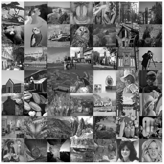
Figure 1. Complete image dataset; 49 grayscale images of $512\times 512$ px.

As a watermark, we used a digital image (LOGO) of $100\times 100$ px, as is shown in Figure 2a. In addition, we used the image MetaData of the Barbara image in plaintext, as we show in Figure 2b.

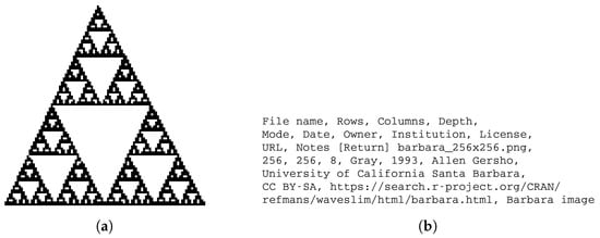
Figure 2. (a) Watermark image LOGO. (b) Image MetaData of the Barbara image in plaintext.

3.2. Jigsaw Transform and Cellular Automata

Image encryption is of great importance currently to ensure the protection of sensitive information by preventing unauthorized access to it. Cryptography techniques used for image encryption are required to have features such as hiding the visual information of the image, having a large key space to resist brute force attacks, and having high key sensitivity to prevent differential attacks [41]. A recent example of an algorithm that meets these requirements is that proposed by Sambas et al. [42], where they developed a three-dimensional chaotic system with line equilibrium, which was used along with Josephus traversal to implement an image encryption scheme based on pixel and bit scrambling and pixel value diffusion, resulting in an encryption method secure against brute force attacks and differential attacks. In addition, the authors implemented the proposed chaotic system into an electronic circuit. In contrast, in the present work, we used the Jigsaw transform and a cellular automaton to encrypt the watermarked image, improving the key space of the Jigsaw-transform-alone implementation.

3.2.1. Jigsaw Transform

The Jigsaw transform is a popular scrambling technique to hide visual information in digital images. Its name is reminiscent of an image cut into pieces of different sizes that must be joined correctly to form the picture again. It is considered a nonlinear operator, which rearranges sections of an image following a random ordering [43]. The direct JST breaks a grayscale image into $\mathcal{M}$ non-overlapping blocks of $s_1\times s_2$ pixels, each one of which is moved to a location following a random order. In the same way as the direct JST ($J_{\mathcal{M}}<>$), the inverse Jigsaw transform ($J_{\mathcal{M}}^{-1}<>$) uses the initial order of the sections to recover the original image. The JST holds the energy of a grayscale image ($I(x,y)$) and is, therefore, considered a unitary transform (Equation (1)).

$$I(x,y)=J_{\mathcal{M}}^{-1}⟨J_{\mathcal{M}}⟨I(x,y)⟩⟩.$$

(1)

Figure 3 shows a grayscale image of $512\times 512$ px and the corresponding results for the JST, giving $\mathcal{M}$ non-overlapping blocks of $64\times 64$ px for $\mathcal{M}=64$, $32\times 32$ px for $\mathcal{M}=256$, and $8\times 8$ px for $\mathcal{M}=4096$.

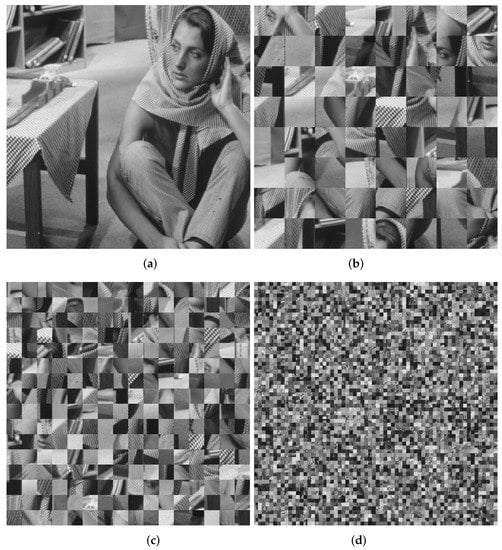
Figure 3. Examples of the JST using an image grayscale image of $512\times 512$ px. (a) Barbara image. (b) JST result using blocks of $64\times 64$ ($\mathcal{M}=64$). (c) JST result using blocks of $32\times 32$ ($\mathcal{M}=256$). (d) JST result using blocks of $8\times 8$ ($\mathcal{M}=4096$).

The set of each possible combination of the security keys used in the encryption of a digital image is called the key space. Thus, for the JST, the key space is related to the number of blocks $\mathcal{M}$, i.e., $K_J=\mathcal{M}!$.

3.2.2. Elementary Cellular Automata

Elementary Cellular Automata consist of a grid of cells of width X and height Y. Each cell has two possible states: ON and OFF. Initially, all cells start turned OFF, except for the first row, which has an arbitrary configuration. The grid will evolve through a series of iterations. In iteration i, the $i+1$th row is modified. The new value of a cell is determined by the neighborhood of the cell in the same column in the row above (the parent row). The neighborhood of a cell consists of three cells: the cell itself and its two horizontal neighbors (handling the edge cases with modular arithmetic). Therefore, there are $2^3=8$ possible neighborhoods and, consequently, $2^8=256$ possible rules for the next iteration of the automaton. In this paper, we focused on the rule known as Rule 105 according to the Wolfram code described in [44] to classify the rules of the ECA, depicted in Figure 4.

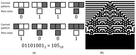
Figure 4. Elementary cellular automaton with Rule 105. (a) The new state of a cell is based on each possible neighborhood of the cell in the same column in its parent row. (b) ECA is applied on a $50\times 51$ grid using 34 iterations, with the first row starting with all cells in the OFF state, except for the cell at the center.

For the purposes of our work, we considered a variant of the ECA, where cells can have values ranging from 0 to an integer k, and instead of using Rule 105 to determine if a cell should be ON or OFF, we used it to determine if a cell should increase its value by an odd number n or not (changing its parity) based on the parity of the values of the corresponding neighborhood, considering even cells as OFF states and odd cells as ON states. If the new value is greater than k, we made use of modular arithmetic to return it to our desired range of values. We also considered a finite grid in the vertical direction; if we performed a number of iterations greater than the amount of rows and we ran out of rows to modify, we continued with the top row considering the bottom row as its parent row. This allowed us to start the first iteration in the first row and to easily apply elementary cellular automata to the gray images. In Figure 5, we show this variation of Rule 105 on a gray image. The process is reversible by applying the algorithm to the rows in reverse order and subtracting by k. The exact size of the key space of our ECA is unknown; its upper bound must be $Y\times k^{X\times Y}$ since that is the total amount of configurations the matrix could have considering all possible values of the matrix and all possible rows that can be modified in a given iteration of the automaton. Evolving the ECA beyond that amount of iterations would lead to a repeated state. Since it is likely that a repeated state will occur before that amount of iterations, the key space of our ECA was $K_{CA}\le Y\times k^{X\times Y}$.

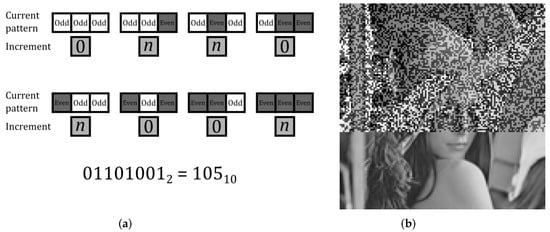
Figure 5. Variation of the ECA with Rule 105. (a) Increment on the value of a cell based on each possible neighborhood of the cell in the same column in its parent row. (b) Our modified ECA was applied on a $128\times 128$ gray image using 80 iterations, with $k=157$.

3.2.3. ECA Applied on Jigsaw Transform

For our work, we used the Jigsaw transform in combination with the elementary cellular automaton described in Section 3.2.2. Given that the JST has a limited key space, the ECA previously described was used to help achieve a broader key space. We used the JST with $\mathcal{M}=5\times 5$ subsections, storing the index of each subsection in a $5\times 5$ matrix to be able to reverse the algorithm. We can encrypt this matrix using our ECA with an arbitrary number of iterations and considering values in the range from 1 to 25. We chose a value of $k=17$ for our work. The key space of the ECA applied on the Jigsaw transform would be $K=(\mathcal{M}!)\left(Y\right)\left(k^{X\times Y}\right)$ in general; substituting for the variables we chose for our work, we obtained a key space of $K\le (25!)\left(5\right)\left({25}^{5\times 5}\right)=1.2689\times {10}^{89}$. We used this algorithm to encrypt our watermark image, as described later in Section 4; given that we used $5\times 5$ subsections, we can achieve full image encryption of the watermark image by using the JST along with 5 iterations of the ECA to modify all the rows of the JST index matrix. Since the main theme of this work was watermarking, a thorough analysis of the JST with the ECA for image encryption is beyond the scope of this article but can be studied in future work.

3.3. SVD Analysis

Singular-value decomposition, used in linear algebra, performs an expansion of a rectangular matrix $A\in {\mathbb{R}}^{M\times N}$ in a coordinate system where M and N are the dimensions of A and the covariance matrix is diagonal. Equation (2) shows the SVD theorem:

$$\begin{array}{cc}\hfill & A=US{V}^T\hfill \\ \\ \hfill & \begin{array}{c}{\mathit{A}}_{\mathit{M}\times \mathit{N}}\\ \left[\begin{array}{ccc}{a}_{11}& \dots & a_{1n}\\ & & \\ & \ddots & \\ & & \\ a_{m1}& \dots & a_{mn}\end{array}\right]\end{array}=\hfill \\ \\ \hfill & \begin{array}{c}{\mathit{U}}_{\mathit{M}\times \mathit{M}}\\ \left[\begin{array}{ccc}{u}_{11}& \dots & u_{m1}\\ & & \\ & \ddots & \\ & & \\ u_{1m}& \dots & u_{mm}\end{array}\right]\end{array}\begin{array}{c}{\mathit{S}}_{\mathit{M}\times \mathit{N}}\\ \left[\begin{array}{ccccc}{\sigma }_1& & \dots & & 0\\ & \ddots & & & \\ & & {\sigma }_r& & \\ & & & \ddots & \\ 0& & \dots & & 0\end{array}\right]\end{array}\begin{array}{c}{\mathit{V}}_{\mathit{N}\times \mathit{N}}\\ \left[\begin{array}{ccc}{v}_{11}& \dots & v_{1n}\\ & & \\ & \ddots & \\ & & \\ v_{n1}& \dots & v_{nn}\end{array}\right]\end{array},\hfill \end{array}$$

(2)

where $U\in {\mathbb{R}}^{M\times M}$ and $V\in {\mathbb{R}}^{N\times N}$ are orthogonal matrices defined by:

$$\begin{array}{c}\hfill U^{T}U=I_{M\times M}\\ \hfill V^{T}V=I_{N\times N}.\end{array}$$

$S\in {\mathbb{R}}^{M\times N}$ is a diagonal matrix, and ${\sigma }_i$ with $i=1,\dots ,M$ are the singular values that satisfy ${\sigma }_1\ge {\sigma }_2\ge \cdots \ge {\sigma }_r={\sigma }_{r+1}=\cdots {\sigma }_{M\times N}=0$ with $r\le M\times N$ representing the rank of the matrix A.

Thus, SVD calculates the eigenvalues of $A{A}^T$, forming the columns of V and the eigenvectors of $A^{T}A$ and generating the columns of U, and the singular values in S are obtained by the square roots of the eigenvalues from $A{A}^T$ and $A^{T}A$.

SVD has been successfully used for a variety of applications. In particular, in the signal- and image-processing areas, SVD has been applied to image compression and image completion [45], dimensionality reduction, facial recognition, background video removal, image noise reduction, cryptography, and digital watermarking [46].

In the following, we describe some properties of SVD:

• A few singular values contain the majority of the signal’s energy, which has been exploited in compression applications.
• The decomposition/reconstruction could be applied to both square and non-square images.
• When a slight interference, e.g., noise, alters the values of the image, the singular values remain relatively stable.
• Singular values of an image represent its intrinsic algebra.

SVD generates the sorted matrices U, S, and V, following how they contribute to the matrix A. Thus, we obtained an approximation of the input image when only a number k of singular values was used. In addition, if k is very near M, the quality of the reconstructed image increases. From Equation (2), an image approximation is obtained taking r columns of U and V and the upper left $r\times r$ square of S.

Figure 6 shows the image approximation using SVD over a grayscale image of $256\times 256$ for $r=8,32,64,128,256$, and Table 1 reports the correlation coefficient (R), which is calculated using the original image and the reconstructed image, where using only $25\%$ of the singular values ($r=64$ of 256), a correlation value of $0.994$ is achieved. In addition, Figure 7 shows the zooming of a region of the original image, where both homogeneous and texture regions are presented.

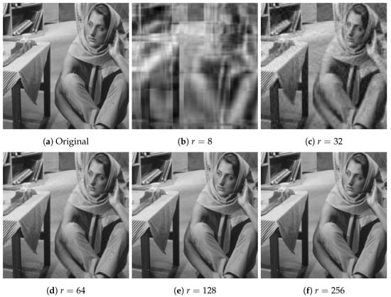
Figure 6. Image approximation using a different number of singular values (r) of SVD.

Table 1. Examples showing the relation between the number of singular values (r) used to reconstruct the image and the correlation coefficient value obtained.

r	R
8	0.903
32	0.981
64	0.994
128	0.999
256	1

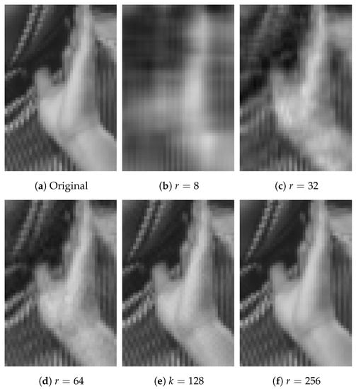
Figure 7. Zoom of the image approximation using a different number of singular values (r) of SVD.

3.4. Hamming Code

Linear block codes, defined in coding theory, are a kind of error-correcting code, where a linear combination of codewords is also a codeword. Hamming codes are efficient error-correcting binary linear block codes used to detect and correct errors when data are stored or transmitted.

For a $(7,4)$ Hamming code, the encoding operation is performed by the $4\times 7$ generator matrix shown in Equation (3) [47]:

$$G=\left[\begin{array}{ccccccc}1& 1& 0& 1& 0& 0& 0\\ 0& 1& 1& 0& 1& 0& 0\\ 0& 0& 1& 1& 0& 1& 0\\ 0& 0& 0& 1& 1& 1& 0\end{array}\right].$$

(3)

When we talk about a $(7,4)$ Hamming code, we are referring to a code that generates seven bits for four input bits. Through a combination, e.g., lineal, of rows of G and the modulo-2 computation, the codewords are obtained for each input element, where the code corresponds to the length of a row of the matrix G. Thus, $\overrightarrow{c}=\overrightarrow{m}G$ is the codeword for $\overrightarrow{m}=\left[\begin{array}{cccc}{m}_1& m_2& m_3& m_4\end{array}\right]$ as the input message [47].

For the decoding process, the $(7,4)$ Hamming code has associated with it a $3\times 3$ parity check matrix H, with $\overrightarrow{v}{H}^T=0$ if $\overrightarrow{v}$ is a codeword. Thus, for the matrix G of Equation (3), the corresponding parity check matrix H is given by Equation (4):

$$H=\left[\begin{array}{ccccccc}\overrightarrow{h_1}& \overrightarrow{h_2}& \overrightarrow{h_3}& \overrightarrow{h_4}& \overrightarrow{h_5}& \overrightarrow{h_6}& \overrightarrow{h_7}\end{array}\right]=\left[\begin{array}{ccccccc}1& 0& 1& 1& 1& 0& 0\\ 0& 1& 0& 1& 1& 1& 0\\ 0& 0& 1& 0& 1& 1& 1\end{array}\right],$$

(4)

where $\overrightarrow{h_k}$ is the column vector k, and it can be verified that $G{H}^T=0$.

3.5. Discrete Cosine Transform

The DCT serves as the foundation for numerous image compression techniques and lossy digital image compression systems: Joint Photographic Experts Group (JPEG) for still images and Moving Picture Experts Group (MPEG) for video images [48]. It is a mathematical tool to perform frequency analysis without complex numbers and to approximate a typical signal using fewer coefficients (low-, high-, and middle-frequency components), i.e., it can pack the most information in the fewest coefficients and pack energy in the low-frequency regions [49,50]. One of the most-usual applications is in signal and image processing for lossy compression because of its property to compact strong energy, creating predictions according to its local uniqueness. Besides, as mentioned in [51], this transform has entropy retention, decorrelation, and energy retention–energy concentration, among which energy concentration is of great significance to digital image encryption. Therefore, the most-important DCT advantages, such as a high compression ratio and low error rates [52], are taken into account in different applications, such as digital image encryption, because the energy concentration is a very important element. When we applied the DCT to an image (matrix), we obtained a DCT coefficient matrix that contained the DC coefficient and the AC coefficient. The energy was concentrated in the DC element. As an example, the Lena image and its transformation applying the DCT are shown in Figure 8.

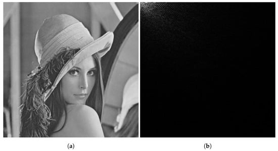
Figure 8. Discrete cosine transform. (a) Original Lena image; (b) DCT of Lena image.

Another application is in steganography systems and watermark systems, which embed the information of a signal in the transform domain. These systems are more robust if they operate in the transform domain (Discrete Fourier Transform (DFT), Discrete Cosine Transform (DCT), Discrete Wavelet Transform (DWT), Contourlet Transform (CT), etc.). Specifically, in the DCT domain, the algorithms are more robust against common processing operations (JPEG and MPEG compression) compared with spatial domain techniques, and also, the DCT offers the possibility of directly realizing the embedding operator in the compressed domain (i.e., inside a JPEG or MPEG encoder) to minimize the computation time [53].

The 2D DCT of a grayscale image $I(x,y)$ is as follows (Equation (5)):

$$I(u,v)=\sum _{y=1}^Y\sum _{x=1}^{X}w(u,v)I(x,y)cos\left(\frac{(2x-1)(u-1)\pi }{2M}\right)cos\left(\frac{(2y-1)(v-1)\pi }{2N}\right),$$

(5)

where X represents the number of columns and Y the number of rows of the image $I(x,y)$, $x,y$ its spatial coordinates, $u,v$ the corresponding frequency coordinates, and

$$w(u,v)=\left\{\begin{array}{cc}\frac{1}{\sqrt{XY}}\hfill & \mathrm{when}u=1,v=1\hfill \\ \sqrt{\frac{2}{XY}}\hfill & \mathrm{when}u=1,v\ge 2\hfill \\ \sqrt{\frac{4}{XY}}\hfill & \mathrm{otherwise},\hfill \end{array}\right.$$

where $w(u,v)$ is a weight factor, $y,v\in [1,\dots ,Y]$ and $x,u\in [1,\dots ,X]$ [54].

The 2D Inverse Discrete Transform (IDCT) is given as follows (Equation (6)):

$$I(x,y)=\sum _{v=1}^Y\sum _{u=1}^{X}w(u,v)I(u,v)cos\left(\frac{(2x-1)(u-1)\pi }{2X}\right)cos\left(\frac{(2y-1)(v-1)\pi }{2Y}\right).$$

(6)

3.6. Hermite Transform

The Cartesian Hermite transform is a technique of signal decomposition. To analyze the visual information, it is necessary to use a Gaussian window function $v^2(x,y)=\frac{1}{\sigma \sqrt{\pi }}exp(-\frac{x^2+y^2}{2{\sigma }^2})$.

The information within the window is expanded to a family of polynomials $G_{o,p-o}(x,y)$. These polynomials have the characteristic of orthogonality in the function of the Gaussian window and are defined in terms of the Hermite polynomials as Equation (7):

$$G_{o,p-o}(x,y)=\frac{1}{\sqrt{2^{p}o!(p-o)!}}{H}_o\left(\frac{x}{\sigma }\right)H_{p-o}\left(\frac{y}{\sigma }\right),$$

(7)

where o and $(p-o)$ indicate the analysis order in the spatial directions x and y, respectively, $p=0,\cdots ,\infty$ and $o=0,\dots ,p$, $H_p$ are the generalized Hermite polynomials, and ${\sigma }^2$ represents the variance of the Gaussian window.

Equation (8) defines the Hermite polynomials.

$$H_p\left(\frac{x}{\sigma }\right)={(-1)}^{p}exp\left(-\frac{x^2}{{\sigma }^2}\right)\frac{d^p}{{\mathit{dx}}^p}exp\left(-\frac{x^2}{{\sigma }^2}\right).$$

(8)

Convoluting the image $I(x,y)$ with the Hermite analysis filters $D_{o,p-o}(x,y)$ followed by a sub-sampling (T) as follows in Equation (9), we obtained the HT.

$$I_{o,p-o}(x_0,y_0)={\int }_{-\infty }^{\infty }{\int }_{-\infty }^{\infty }I(x,y)D_{o,p-o}(x_0-x,y_0-y)dxdy,$$

(9)

where $I_{o,p-o}(x,y)$ are the Cartesian Hermite coefficients:

$$D_{o,p-o}(x,y)=G_{o,p-o}(-x,-y)v^2(-x,-y),$$

and $(x_0,y_0)$ is the spatial position in the sampling lattice S.

The Hermite filters are obtained by Equation (10):

$$D_k\left(x\right)=\frac{{(-1)}^k}{\sqrt{2^{k}k!}}\frac{1}{\sigma \sqrt{\pi }}{H}_k\left(\frac{x}{\sigma }\right)exp\left(-\frac{x^2}{{\sigma }^2}\right),$$

(10)

with $k=0,1,2,\dots ,\infty$.

On the other hand, the original image could be reconstructed through Equation (11):

$$I(x,y)=\sum _n^{\infty }\sum _{p=0}^n\sum _{(x_0,y0)\in S}{I}_{o,p-o}(x_0,y_0)·P_{o,p-o}(x-x_0,y-y_0),$$

(11)

where $P_{o,p-o}$ are the Hermite synthesis filters of Equation (12) and $V(x,y)$ is the weight function of Equation (13).

$$P_{o,p-o}(x,y)=\frac{D_{o,p-o}(x,y)}{V(x,y)}.$$

(12)

$$V(x,y)=\sum _{(x_0,y_0)\in S}{v}^2(x-x_0,y-y_0)\ne 0.$$

(13)

For the discrete implementation, we used the binomial window function to approximate the Gaussian window function (Equation (14)):

$${\omega }^2\left(x\right)=\frac{1}{2^{\mathcal{N}}}{C}_{\mathcal{N}}^x,x=0,1,\dots ,\mathcal{N}-1,\mathcal{N},$$

(14)

where $\mathcal{N}$ represents the order of the binomial window (Equation (15)).

$$C_{\mathcal{N}}^x=\frac{\mathcal{N}!}{(\mathcal{N}-x)!}x!,x=0,1,\dots ,\mathcal{N}-1,\mathcal{N}.$$

(15)

Thus, the Krawtchouk polynomials, defined in Equation (16), are the orthogonal polynomials $G_{o,p-o}(x,y)$ associated with the binomial window.

$$K_n\left[x\right]=\frac{1}{\sqrt{\phantom{(}{C}_{\mathcal{N}}^n}}\sum _{k=0}^n{(-1)}^{n-k}{C}_{\mathcal{N}-x}^{n-k}{C}_x^k.$$

(16)

In the discrete implementation, the signal reconstruction from the expansion coefficients is perfect because the window function support is finite ($\mathcal{N}$) and the expansion with the Krawtchouk polynomials is also finite. To implement the Hermite transform, it is necessary to select the size of the Gaussian window spread $\left(\sigma \right)$, the order $\mathcal{N}$ for binomial windows, and the subsampling factor that defines the sampling lattice S. The resulting Hermite coefficients are arranged as a set of ($\mathcal{N}\times \mathcal{N}$) equally sized sub-bands: one coarse sub-band $I_{0,0}$ representing a Gaussian-weighted image average and detail sub-bands $I_{n,m}$ corresponding to higher-order Hermite coefficients, as we can see in Figure 9.

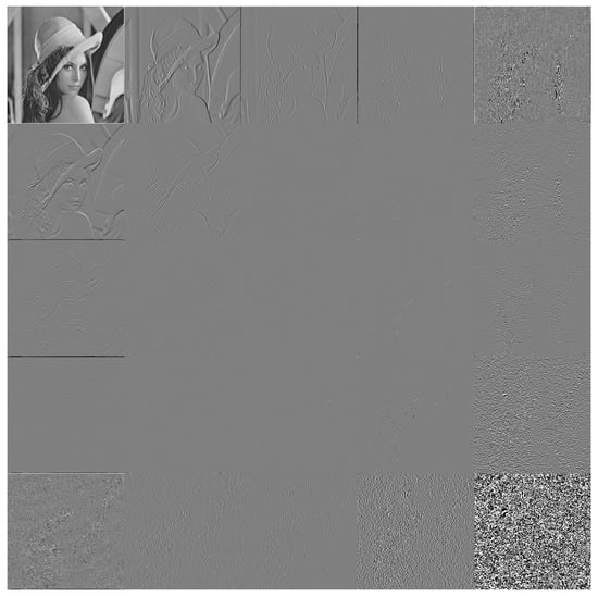
Figure 9. Hermite transform coefficients ($L_{o,p-o}(x,y)$ with $N=4$) of Lena image and the spatial order representation: $(o,p-o)=\left[\begin{array}{ccccc}0,0& 1,0& 2,0& 3,0& 4,0\\ 0,1& 1,1& 2,1& 3,1& 4,1\\ 0,2& 1,2& 2,2& 3,2& 4,2\\ 0,3& 1,3& 2,3& 3,3& 4,3\\ 0,4& 1,4& 2,4& 3,4& 4,4\end{array}\right]$.

3.7. Human Vision System

For several years, some characteristics of the HVS have been applied to address various image-processing challenges. For example, in [55], the authors proposed a watermarking approach considering that the determined mechanisms of the HVS are less sensitive to the redundancy of image information. Thus, the entropy was used to determine the regions with more redundant image information and to select the visually significant embedding regions.

On the other hand, entropy is a metric widely used to measure the spatial correlation of a local region of the image, for example a pixel neighborhood. It could be defined for an N-state, as is shown in Equation (17) [55]:

$$E=-\sum _{j=1}^N{p}_j{log}_2\left(p_j+ϵ\right),$$

(17)

where $p_j$ defines the probability of the appearance of the $j-th$ pixel in the pixel neighborhood, N is the number of elements within the neighborhood, and $ϵ\ll 1$ is a small constant value to avoid ${log}_2\left(0\right)$.

In addition, image edges contain relevant information about the image characteristics. Thus, the edge entropy of an image block is taken into consideration to identify the specific areas in the image where the watermark will be inserted. It is calculated by means of Equation (18) [55]:

$$E_{edge}=-\sum _{j=1}^N{p}_j{exp}_2^{\left(1-p_i\right)},$$

(18)

where $1-p_j$ represents the uncertainty of the j-th pixel value in the block.

In [55], the combination between the entropy and edge entropy was used to determine the suitable insertion locations, as is shown in Equation (19):

$$\mathrm{HVS}=\sum _{j=1}^N\left[]p_j{log}_2\left(p_j+ϵ\right)-p_j{exp}_2^{\left(1-p_j\right]}\right).$$

(19)

4. Proposed HT, DCT, and SVD and Block-Based Watermarking Method

The present work reports a blockwise image watermarking method to insert two watermarks, a digital image (LOGO) and information about the owner or the host image (MetaData). The proposed method is based on the HT and DCT as a spatial–frequency representation of the cover image with the HVS characteristics to add imperceptibility to the watermark. In addition, an SVD strategy adds robustness against attacks.

4.1. Watermarking Insertion Process

Figure 10 shows a schema of the proposed watermarking insertion process.

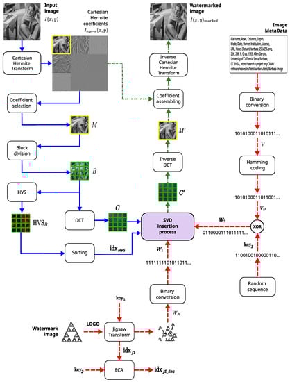
Figure 10. Watermarking insertion process.

The reason to use DCT is that, according to Dowling et al. [56], block-based watermarking is more effective because we have smaller block sizes and the DCT concentrates the energy. After decomposing the original image into space–frequency bands using the HT, the selected sub-bands were partitioned into 4 × 4 blocks. Subsequently, each block was transformed into its DCT representation. On the one hand, an SVD analysis allows high robustness against attacks. On the other hand, the entropy values of the cover image are used to choose the suitable regions for embedding the watermarks, giving an adaptive approach that identifies blocks with high entropy. Thus, $\mathrm{HVS}$ values (Equation (19)) in each block are sorted in ascending order, where the lowest values correspond to the best embedding regions. Figure 11a shows a grayscale image of $512\times 512$ px, and Figure 11b represents through a color bar, with descending and normalized values, those regions where a watermark, in this case of $100\times 100$ px, could be inserted, where high values (light color) correspond to the most-suitable regions and low values (dark color) are the worst regions.

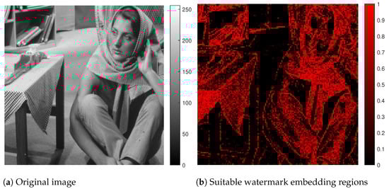
Figure 11. Embedding regions to insert a watermarking using the HVS values. (a) Grayscale original image. (b) The suitable regions to insert a watermark in descending order. Best locations (light color) and worst ones (dark color).

In addition, to increase the performance of the image MetaData against attacks and reduce channel distortion, a $(7,4)$ Hamming error-correcting code was applied to the MetaData. Finally, the LOGO image was encrypted using the Jigsaw transform in combination with elementary cellular automata to increase the security of the proposal.

The steps of embedding both an image watermark (LOGO) ($W_1$) and the image MetaData ($W_2$) are explained next regarding the block diagram of Figure 10:

• Image watermark (LOGO) $W_1$:

  –

  Input the binary image watermark LOGO of size $k_1\times k_2$.

  –

  Apply the Jigsaw transform to the LOGO with ${\mathrm{key}}_1=\mathcal{M}$ as the first secret key, obtaining the watermark matrix $W_A$ of size $k_1\times k_2$, where $\mathcal{M}$ corresponds to the number of non-overlapping subsections of $s_1\times s_2$ px.

  –

  Convert $W_A$ to binary, obtaining the sequence $W_1\in {\mathbb{R}}^{1\times L_{bin}}$.

  –

  The Jigsaw transform generates the indexes $id{x}_{JS}$, which represent the original locations of each subsection of $s_1\times s_2$ px.

  –

  The ECA algorithm encrypts $id{x}_{JS}$ through ${\mathrm{key}}_2$, obtaining the encrypted indexes ${\mathrm{idx}}_{JS\_Enc}$, where ${\mathrm{key}}_2=\left[\begin{array}{cc}{N}_{ite}& \\ k\end{array}\right]$ is the second secret key, with $N_{ite}$ representing the number of iterations, and k is an odd number.

• Image MetaData $W_2$:

  –

  Enter the image MetaData as a character string.

  –

  Convert each alphanumeric character of the image MetaData into a binary string, obtaining the vector V.

  –

  Calculate the $(7,4)$ Hamming code over V, obtaining the vector $V_H$ of length P.

  –

  Generate a pseudo-random binary string $k_r$ of length P with a uniform distribution; ${\mathrm{key}}_3=k_r$ will be the third secret key.

  –

  Perform the bitwise operation to obtain the watermark $W_2$:

  $$W_2=\left(V_H\right)\mathrm{XOR}\left({\mathrm{key}}_3\right).$$

  (20)

  –

  Since the image MetaData size is small compared tothe LOGO image size, an adjustment of the dimensions of $W_2$ by adding binary zeros to correspond to the dimensions of $W_1\in {\mathbb{R}}^{1\times L_{bin}}$ is performed.

• Input host image to watermark:

  –

  Input the host image. For an RGB image, convert it to grayscale, obtaining a matrix $I(x,y)$ of size $m_1\times n_1$.

  –

  Perform the Hermite transform decomposition to $I(x,y)$, to obtain nine coefficients. Each one is a matrix $I_{o,p-o}(x,y)$ of size $m_2\times n_2$, where $m_2=\frac{m_1}{T}$ and $n_2=\frac{n_1}{T}$, where T is a sub-sampling factor, e.g., $T=2$.

  –

  Select the low-spatial-frequency Hermite coefficient $M=I_{0,0}$ to embed the watermarks $W_1$ and $W_2$.

  –

  Divide M into blocks of size $b\times b$, obtaining the multidimensional array B composed of $L=\frac{m_2}{b}\times \frac{n_2}{b}$ blocks.

  –

  Apply the HVS analysis to each block of matrix B through Equation (19), obtaining ${\mathrm{HVS}}_B$.

  –

  Sort each value of ${\mathrm{HVS}}_B$ in ascending order, storing the position ${\mathrm{idx}}_{HVS}$ of each ordered block, where the lowest values of ${\mathrm{HVS}}_B$ correspond to the best embedding regions.

  –

  Apply the DCT to each block of B, obtaining $C=\mathrm{DCT}\left\{B\right\}$, where $C\in {\mathbb{R}}^{b\times b\times L}$ and L is the number of blocks of size $b\times b$.

• SVD-based insertion process:

  –

  Embed the watermarks $W_1$ and $W_2$ using the SVD-based Algorithm 1, with blocks of $b\times b=4\times 4$, obtaining the multidimensional output array $C^{\prime }$.

  –

  To fully embed the LOGO and image MetaData within the host image, the following relation must be satisfied:

  $$L_{bin}\le L.$$

  (21)

• Making the watermarking image:

  –

  Apply the inverse DCT to each block of $C^{\prime }$, obtaining $M^{\prime }={\mathrm{DCT}}^{-1}\left\{C^{\prime }\right\}$.

  –

  Substitute the low-spatial-frequency Hermite coefficient of $I_{o,p-o}(x,y)$: $I_{0,0}(x,y)=M^{\prime }$.

  –

  Perform the inverse Hermite transform of $I_{o,p-o}(x,y)$ to obtain $I{(x,y)}_{\mathrm{marked}}$.

Algorithm 1: SVD-based insertion algorithm.

4.2. Watermarking Extraction Process

Since the watermarking approach is symmetric, the extraction stage is similar to the process shown in Figure 10, with the only change that the inverse operations are applied. Thus, the steps of extracting both the LOGO and the plaintext MetaData from the watermarked image are explained next:

• SVD-based extraction process:

  –

  Perform the Hermite transform decomposition to $I{(x,y)}_{\mathrm{marked}}$.

  –

  Select the low-spatial-frequency Hermite coefficient $M=I_{0,0}$.

  –

  Divide M into blocks of size $4\times 4$, obtaining the multidimensional array B composed of L blocks.

  –

  Apply the DCT to each block of B, obtaining $C=\mathrm{DCT}\left\{B\right\}$.

  –

  Extract the matrices $W_1$ and $W_2$ using the SVD-based Algorithm 2.

• LOGO image extraction:

  –

  Convert array $W_1\in {\mathbb{R}}^{1\times L_{bin}}$ into a matrix $W_A\in {\mathbb{R}}^{k_1\times k_2}$.

  –

  Decrypt $id{x}_{JS}$ through the inverse ECA using ${\mathrm{key}}_2=\left[\begin{array}{cc}{N}_{ite}& \\ k\end{array}\right]$, obtaining $id{x}_{JS}$ indexes.

  –

  Apply the inverse JST to $W_A$ using $id{x}_{JS}$ indexes to obtain the LOGO image.

• Image MetaData extraction:

  –

  Remove the extra zeros of $W_2\in {\mathbb{R}}^{1\times L_{bin}}$ to obtain the array $W_2^{\prime }\in {\mathbb{R}}^{1\times P}$.

  –

  Perform the bitwise operation between $W_2^{\prime }$ and ${\mathrm{key}}_3$ to obtain $V_H$:

  $$V_H=\left(W_2^{\prime }\right)\mathrm{XOR}\left({\mathrm{key}}_3\right).$$

  (22)

  –

  Decode $V_H$ using the $(7,4)$ Hamming code to obtain the binary array V.

  –

  Convert the binary array V to an alphanumeric array, obtaining the the image MetaData as a character string.

Algorithm 2: SVD-based extraction algorithm.

5. Experiments and Results

The proposed watermarking method was run on a laptop computer with an Intel Core i7 @ 1.6 GHz, 16 GB of RAM, and without a GPU card. The watermarking algorithm had a time consumption of 2.971 s for the insertion stage and 2.640 s for the extraction process. The method was implemented in a non-optimized and non-parallelized script in MATLAB using images of $512\times 512$ px. The parameters used were $s_1=s_2=100$ for the JST, $\mathcal{N}=2$, maximum order decomposition $D=4$ and $T=1$ for the HT, $N_{ite}=275$ and $k=17$ for the ECA, $b\times b=4\times 4$ for the HVS analysis, and $\alpha =0.00001$ for the SVD-based insertion.

We evaluated our algorithm in different experiments: the insertion and extraction processes, robustness against attacks, and a comparison with other methods.

All the experiments were carried out using the 49 publicly available grayscale images of $512\times 512$ px (see Section 3.1).

5.1. Performance Measures

To assess the performance of our watermarking algorithm, we employed the following metrics [53]: Mean-Squared Error (MSE), Peak Signal-to-Noise Ratio (PSNR), Structural Similarity Index (SSIM), Mean Structural Similarity Index (MSSIM), Normalized Cross-Correlation (NCC), Bit Error ($B_{error}$), and Bit Error Rate (BER). In the cases of the MSE, PSNR, SSIM, MSSIM, and NCC, the images were $X\times Y$ px, where x and y represent the spatial coordinates:

• The MSE refers to a statistical metric used to measure the image’s quality. It evaluates the squared difference between a pixel in the original image $I_1$ and the watermarked image $I_2$. After calculating this result for all pixels in the image, it returns the average result, as is shown in Equation (23):

  $$MSE=\frac{1}{XY}\sum _{x=1}^X\sum _{y=1}^Y{\left[I_1(x,y)-I_2(x,y)\right]}^2.$$

  (23)
  If the MSE = 0, this indicates that there is no error between the original image and the watermarked image.
• The PSNR is defined in Equation (24):

  $$PSNR=10{log}_{10}\left(\frac{{255}^2}{MSE}\right).$$

  (24)
  On the one hand, a higher image quality is achieved with a higher PSNR value, so it approaches infinity. On the other hand, low PSNR values report high differences between the images [57].
• The Mean Structure Similarity Index (MSSIM) has a value determined by Equation (25):

  $$MSSIM(I,\widehat{I})=\frac{1}{M}\sum _{j=1}^{M}SSIM(I_j,{\widehat{I}}_j),$$

  (25)

  where I and $\widehat{I}$ correspond to the original and the distorted image, respectively, $I_j$ and ${\widehat{I}}_j$ represent their j-th local window, and M stands for the amount of local windows of the image. In the case that $I_j$ and ${\widehat{I}}_j$ have no negative values, the value of the SSIM is calculated as shown in Equation (26):

  $$SSIM(I,\widehat{I})=\frac{(2{\mu }_I{\mu }_{\widehat{I}}+C_1)(2{\sigma }_{I\widehat{I}}+C_2)}{({\mu }_I^2+{\mu }_{\widehat{I}}^2+C_1)({\sigma }_I^2+{\sigma }_{\widehat{I}}^2+C_2)},$$

  (26)

  where the averages of I and $\widehat{I}$ are given by ${\mu }_I$ and ${\mu }_{\widehat{I}}$, respectively, their standard deviations are given by ${\sigma }_I$ and ${\sigma }_{\widehat{I}}$, the covariance between both images is represented by ${\sigma }_{I\widehat{I}}$, and the constants $C_1$ and $C_2$ are used to prevent instability if the denominator happens to have a value close to zero [58].
  The SSIM is a metric that quantifies the similarity between two images and is believed to correlate with the quality perception of the human visual system [57]. The SSIM ranges in the interval $[0,1]$. Thus, close to zero values indicate uncorrelated images, and values closer to 1 represent equal images.
• The Normalized Cross-Correlation coefficient (NCC) measures the amount of similarity between two images ($I_1$ and $I_2$) given their gray level intensities, as illustrated by Equation (27):

  $$NCC=\frac{{\displaystyle \sum _x^X}{\displaystyle \sum _y^Y}\left(I_1(x,y)-{\overline{I}}_1\right)\left(I_2(x,y)-{\overline{I}}_2\right)}{{\left(\left[{\displaystyle \sum _x^X}{\displaystyle \sum _y^Y}{\left(I_1(x,y)-{\overline{I}}_1\right)}^2\right]\left[{\displaystyle \sum _y^Y}{\displaystyle \sum _y^Y}{\left(I_2(x,y)-{\overline{I}}_2\right)}^2\right]\right)}^{1/2}},$$

  (27)

  where ${\overline{I}}_{*}$ represents the average value of $I_{*}$.
• The Bit error ($B_{error}$) denotes the number of wrong bits extracted from the binary string $\widetilde{\left(W\right)}\left(x\right)$, regarding the total bits (N) embedded in the binary string $W\left(x\right)$ [53].
• The Bit Error Rate (BER) is similar to the bit error, but it measures the ratio between the number of wrong bits extracted from the binary string $\widetilde{\left(W\right)}\left(x\right)$, regarding the total bits (N) embedded in the binary string $W\left(x\right)$ [53] (see Equation (28)):

  $$BER=\frac{\sum |W\left(x\right)-\widetilde{\left(W\right)}\left(x\right)|}{N}.$$

  (28)

5.2. Sensitivity Analysis of the Scaling Factor

A critical parameter in the proposed SVD-based watermarking method (see Algorithm 1) corresponds to the scaling factor $\alpha$. This parameter defines the imperceptibility, on the one hand, and robustness, on the other, of the proposed watermarking method. A low value ensures imperceptibility, but minimizes robustness, while a high value gives strong robustness, but neglects the imperceptibility of the watermarks. Thus, to fix a suitable value of $\alpha$, we performed a sensitivity analysis of the scaling factor by varying $\alpha$ from 10${}^{-6}$ to 10${}^{-3}$ with steps of 10${}^{-6}$, obtaining a set of one-hundred different values. Then, we embedded the watermarks into the Lena image and calculated the performance metrics. Thus, for the watermarked image, we computed the NC and SSIM values; for the extracted LOGO image, the NCC values; and for the image MetaData recovered, the BER values. We obtained an NCC = 1 for the LOGO watermark and a BER = 0 for the image MetaData extracted using the one-hundred values of $\alpha$, which showed that $\alpha$ did not affect the extraction process. However, the NCC and SSIM metrics for the watermarked image showed a behavior dependent on $\alpha$. In Figure 12a, we show a plot of the NCC (solid red line) and SSIM (dashed blue line) values of the watermarked image as a function of $\alpha$, where both metrics decreased when $\alpha$ increased. Then, Figure 12b shows an enlargement of the left-upper rectangle region (black dotted line) of Figure 12a, showing that, for values greater than ${\alpha }_{th}=$ 10${}^{-5}$ (vertical black dotted line), both the NCC and SSIM values decreased considerably. For this, we fixed the scaling factor to $\alpha =$ 10${}^{-5}$ to ensure, on the one hand, the quality of the marked image and, on the other hand, the correct extraction of both watermarks.

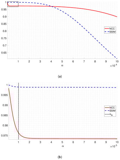
Figure 12. Sensitivity analysis of the scaling factor. (a) NCC (solid red line) and SSIM (dashed blue line) values of the watermarked image versus $\alpha$. (b) Enlargement of the left-upper rectangle region (black dotted line) of (a) showing the defined limit value of $\alpha$.

5.3. Watermarking Insertion and Extraction Performance Analysis

We tested our algorithm on the 49 grayscale images shown in Section 3.1 to insert and extract the LOGO watermark (Figure 2a) and the image MetaData (Figure 2b).

In Table 2, we present the metrics’ averages by applying the algorithm to the 49 grayscale images. In addition, in Table 3, we show only the results using six representative images. However, the results were similar for the other images. As representative images, we selected the following images commonly used to test image-processing algorithms, and at the same time, they represent the variability of both low and high spatial frequencies: Baboon, Barbara, Boat, Cameraman, Lena, and Peppers. The experimental results using these representative images are shown in Figure 13, where each pair shows the original image on the left and the watermarked image on the right.

Table 2. Metrics’ averages using 49 grayscale images, showing the metrics over the watermarked images and the metrics of the LOGO and MetaData extracted.

Number of Images	Insertion (Image Watermarked)					Extraction (LOGO and MetaData)
	MSE	PSNR (dB)	NCC	SSIM	MSSIM	MSE	PSNR (dB)	NCC	SSIM	MSSIM	BER
49	7.1710	40.2051	0.9987	0.9999	0.9994	0	≫60	1	1	1	0

Table 3. Metrics’ averages using only six representative images, showing the metrics over the watermarked images and the metrics of the LOGO (MSE, PSNR, NCC, SSIM, MSSIM) and MetaData (BER) extracted.

Image	Insertion (Image Watermarked)					Extraction (LOGO and MetaData)
	MSE	PSNR (dB)	NCC	SSIM	MSSIM	MSE	PSNR (dB)	NCC	SSIM	MSSIM	BER
Baboon	6.1477	40.2436	0.9982	0.9999	0.9999	0	≫60	1	1	1	0
Barbara	7.7169	39.2563	0.9987	0.9999	0.9998	0	≫60	1	1	1	0
boat	8.2219	38.9810	0.9981	0.9999	0.9998	0	≫60	1	1	1	0
Cameraman	9.9479	38.1534	0.9987	0.9998	0.9985	0	≫60	1	1	1	0
Lena	7.9506	39.1267	0.9982	0.9999	0.9994	0	≫60	1	1	1	0
Peppers	5.8028	40.4943	0.9990	0.9999	0.9998	0	≫60	1	1	1	0

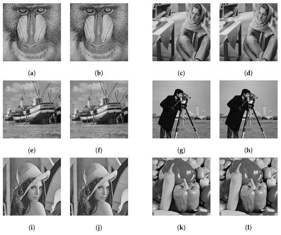
Figure 13. Results of original images and their watermarked images without attack. (a,c,e,g,i,k) correspond to the original images Baboon, Barbara, Boat, Cameraman, Lena, and Peppers, respectively. (b,d,f,h,j,l) correspond to the watermarked images.

Table 2 and Table 3 show, through the values of the metrics (PSNR, MSSIM), that the watermark is visually imperceptible, so both the LOGO and the image MetaData did not present perceptible changes. In relation to the extracted watermark and the MetaData, all metrics demonstrated that we can recover them perfectly. Among the six representative images, the best results were for the Peppers image; after inserting the watermark, the quantity of the pixels modified was 5.8020, and the rest of the metrics demonstrated that there were no visual changes. The Cameraman image presented the highest MSE value and the lowest PSNR value, but also these values indicated that the watermark was not perceptible.

5.4. Watermarking Robustness against Attacks

To evaluate the robustness against attacks of the proposed watermarking method, we applied the most-common processing and geometric attacks to the 49 grayscale watermarked images of Section 3.1.

Processing operations: Gaussian filter and median filter; Gaussian noise and salt and pepper noise. Gaussian filter—window of $N\times N$ and varying N from 2 to 11; median filter—window of $N\times N$, and N varies between 2 and 9; Gaussian noise—with ${\sigma }^2\in [0,0.5]$ and increments of 0.05; SP noise—with noise density varying between 0 and 1 and increments of 0.1. Additionally, we applied image compression and image scaling. JPEG compression—with a variation of the quality factor between 0% and 100% and steps of 10%; Scale—with a scale varying between 0.25 and 4 and steps of 0.25. Furthermore, we applied histogram equalization and contrast enhancement. Equalization—varying the discrete equalization levels 2${}^n$, where n is from 2 to 8. Contrast enhancement—varying f from 0.01 to 0.45 with increments of 0.05, such as suturing the bottom $f\%$ and the top $(1-f\%)$ of all pixel values using the histogram information.

Geometric attacks: Rotation—varying the rotation angle from 1° to 180° with steps of 5°. Translation—the variation was from 10 to 100 px, with increments of 10. Finally, we cropped the watermark image, substituting the original pixels for black pixels. In percentage p was from 0 to 95%. Table 4 shows the metrics’ averages using the 49 grayscale watermarked images for all attacks with parameter variation, including the metrics of the LOGO and MetaData recovered. As we can see, only with the Rotation and the Cropping was it difficult to recover the LOGO and the MetaData. For both cases, the bits modified in the MetaData were significant, and the LOGO images had visual modifications because the PSNR values and the SSIM values were high. With Gaussian noise, SP noise, scale, and contrast enhancement, $BER$ = 0, $PSNR\gg 60$, NCC = 1, SSIM = 1, MSSIM = 1, and MSE = 0, indicating that the recovered watermark was equal to the inserted watermark. In the rest of the attacks (Gaussian filter, median filter, translation, JPEG compression, and histogram equalization), the values of the PSNR, NCC, SSIM, and MSSIM indicated that there was a high similarity between the original watermark and the extracted watermark. In the case of the LOGO image, it could present visual changes, but it was still visible, and the MetaData changed in some characters. It is important to note that, in this table, we included the $BER$ (number of modified bits) and $B_{error}$ (BER ratio) to identify if a LOGO had modified bits. For example, with the Gaussian filter, $BER$ = 0 indicates that the watermark did not have modified bits, but if we calculated the BER ratio ($B_{error}$), it was clear that it had few modifications.

Table 4. Metrics’ averages using 49 grayscale images for all attacks with parameter variation, showing the metrics of the LOGO (MSE, PSNR, NCC, SSIM, MSSIM) and MetaData ($B_{error}$, BER) extracted.

Attack/(Parameter)	Value Range (Step)	MSE	PSNR (dB)	NCC	SSIM	MSSIM	${\mathit{B}}_{\mathit{e}\mathit{r}\mathit{r}\mathit{o}\mathit{r}}$	BER
Gaussian Filter/$(N\times N)$	2 to 11 (1)	0.0398	59.8776	1	1	1	0.0061	0
Median Filter/$(N\times N)$	2 to 9 (1)	1.8910	58.8276	0.9999	0.9991	0.9985	0.5536	0.0001
Gaussian Noise/$\left({\sigma }^2\right)$	0.05 to 0.5 (0.05)	0	≫60	1	1	1	0	0
Salt and Pepper Noise/(density)	0.1 to 1 (0.1)	0	≫60	1	1	1	0	0
Scaling/(scale factor)	0.25 to 4 (0.25)	0	≫60	1	1	1	0	0
Translation/(pixels)	10 to 100 (10)	157.8250	54.3528	0.9934	0.9664	0.9589	16.2102	0.0040
Rotation/(angle ${}^{\circ }$)	1 to 180 (15)	4760.5956	20.6053	0.8262	0.5455	0.5376	185.4662	0.0462
Cropping/($p\%$)	0 to 95 (5)	23,540.7884	8.4022	0.4894	0.2696	0.2636	916.1224	0.2280
Contrast Enhancement/$\left(f\right)$	0.01 to 0.45 (0.04)	0	≫60	1	1	1	0	0
JPEG Compression/$\left(qualityfactor\right)$	100 to 0 (10)	0.4584	59.6741	1.0000	0.9999	0.9998	19.3859	0.0048
Histogram Equalization/(discrete levels)	2${}^n$, n was from 2 to 8	615.0076	43.5160	0.9765	0.9019	0.8826	36.6210	0.0091

To analyze in detail the results of the robustness against attacks, in Table 5, we show the metrics’ averages for all attacks with parameter variation, showing the metrics for the recovery of the LOGO and MetaData extracted after applying the algorithm using only the Lena image. The results for each metric demonstrated that our proposal is robust and imperceptible. In Figure 14, Figure 15 and Figure 16, we present the original Lena image, recovered watermark, and recovery MetaData after applying some attacks. In Figure 14, we can observe that, after applying the median filter, SP noise, and JPEG compression, it was possible to recover the watermark and MetaData. The same result was obtained if we applied histogram equalization and translation (Figure 15). Finally, in Figure 16, we can see that, if we rotate or crop the watermark image, in some cases, it was not possible to recover the watermark and the MetaData without modifications, but in the majority of the cases, we had good results.

Table 5. Metrics obtained from all attacks, with parameter variation, after applying the watermarking algorithm over Lena’s image and showing the metrics of the LOGO (MSE, PSNR, NCC, SSIM, MSSIM) and MetaData ($B_{error}$, BER) extracted.

Attack/(Parameter)	Value Range (Step)	MSE	PSNR (dB)	NCC	SSIM	MSSIM	${\mathit{B}}_{\mathit{e}\mathit{r}\mathit{r}\mathit{o}\mathit{r}}$	BER
Gaussian Filter/$(N\times N)$	2 to 11 (1)	0	≫60	1	1	1	0	0
Median Filter/$(N\times N)$	2 to 9 (1)	0	≫60	1	1	1	0	0
Gaussian Noise/$\left({\sigma }^2\right)$	0.05 to 0.5 (0.05)	0	≫60	1	1	1	0	0
Salt and Pepper Noise/(density)	0.1 to 1 (0.1)	0	≫60	1	1	1	0	0
Scaling/(scale factor)	0.25 to 4 (0.25)	0	≫60	1	1	1	0	0
Translation/(pixels)	10 to 100 (10)	0	≫60	1	1	1	0	0
	1	0	≫60	1	1	1	0	0
	15	4564.7550	11.5366	0.8201	0.4416	0.4326	147	0.0366
	30	7601.4225	9.3219	0.7321	0.3890	0.3843	261	0.0650
	45	8908.4250	8.6328	0.6992	0.3739	0.3699	327	0.0814
	≫60	7724.9700	9.2518	0.7289	0.3909	0.3863	299	0.0744
	75	4493.2275	11.6052	0.8224	0.4436	0.4342	172	0.0428
Rotation/(angle ${}^{\circ }$)	90	0	≫60	1	1	1	0	0
	105	4564.7550	11.5366	0.8201	0.4416	0.4326	147	0.0366
	120	7601.4225	9.3219	0.7321	0.3890	0.3843	261	0.0650
	135	8908.4250	8.6328	0.6992	0.3739	0.3699	327	0.0814
	150	7724.9700	9.2518	0.7289	0.3909	0.3863	299	0.0744
	165	4493.2275	11.6052	0.8224	0.4436	0.4342	172	0.0428
	180	0	≫60	1	1	1	0	0
	5	1703.6550	15.8170	0.9239	0.5595	0.5079	28	0.0070
	10	3290.2650	12.9585	0.8633	0.4735	0.4589	62	0.0154
	15	5806.7325	10.4915	0.7819	0.4225	0.4165	109	0.0271
	20	8973.4500	8.6012	0.6977	0.3772	0.3734	226	0.0562
	25	11,724.0075	7.4400	0.6361	0.3456	0.3425	342	0.0851
	30	14,741.1675	6.4455	0.5775	0.3133	0.3107	475	0.1182
	35	18,011.9250	5.5752	0.5216	0.2777	0.2754	585	0.1456
	40	20,840.5125	4.9417	0.4781	0.2475	0.2453	701	0.1745
	45	23,974.7175	4.3333	0.4338	0.2166	0.2146	829	0.2063
Cropping/($p\%$)	50	27,167.4450	3.7903	0.3919	0.1863	0.1844	967	0.2407
	55	29,989.5300	3.3611	0.3568	0.1589	0.1571	1082	0.2693
	60	33,370.8300	2.8971	0.3163	0.1278	0.1260	1239	0.3084
	65	35,991.3375	2.5688	0.2855	0.1042	0.1025	1348	0.3355
	70	37,766.5200	2.3597	0.2647	0.0892	0.0875	1420	0.3534
	75	40,159.4400	2.0929	0.2363	0.0707	0.0691	1518	0.3778
	80	42,727.9275	1.8237	0.2048	0.0473	0.0458	1637	0.4074
	85	44,685.1800	1.6292	0.1793	0.0341	0.0327	1716	0.4271
	90	47,214.6525	1.3900	0.1431	0.0188	0.0175	1811	0.4507
	95	49,327.9650	1.1999	0.1070	0.0097	0.0086	1891	0.4706
Contrast Enhancement/$\left(f\right)$	0.01 to 0.45 (0.04)	0	≫60	1	1	1	0	0
JPEG Compression/(quality factor)	100 down to 10 (−10)	0	≫60	1	1	1	0	0
	0	0	≫60	1	1	1	189	0.0470
Histogram Equalization/(discrete levels)	4	7822.5075	9.1973	0.7263	0.3872	0.3824	181	0.0450
	8	481.1850	21.3077	0.9772	0.7883	0.6868	15	0.0037
	16	19.5075	35.2288	0.9991	0.9975	0.9971	2	0.0005
	32	6.5025	40	0.9997	0.9994	0.9994	0	0
	64	0	≫60	1	1	1	0	0
	128	0	≫60	1	1	1	0	0
	256	0	≫60	1	1	1	0	0

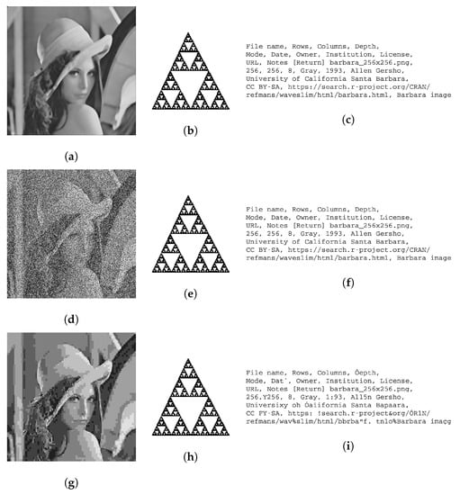
Figure 14. Median filter (9): (a) Filtered Lena image. (b) Recovered watermark (LOGO). (c) Recovered MetaData. SP noise (0.5): (d) Noisy Lena image. (e) Recovered watermark (LOGO). (f) Recovered MetaData. JPEG compression (0): (g) Compressed Lena image. (h) Recovered watermark (LOGO). (i) Recovered MetaData.

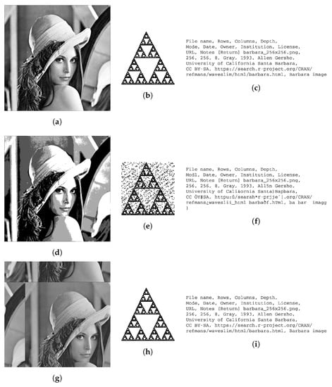
Figure 15. Histogram equalization (128): (a) Equalized Lena image. (b) Recovered watermark (LOGO). (c) Recovered MetaData. Histogram equalization (4): (d) Equalized Lena image. (e) Recovered watermark (LOGO). (f) Recovered MetaData. Translation (100): (g) Translated Lena image. (h) Recovered watermark (LOGO). (i) Recovered MetaData.

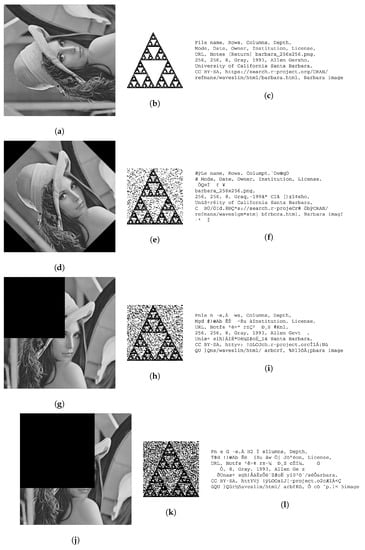
Figure 16. Rotation (90): (a) Rotated Lena image. (b) Recovered watermark (LOGO). (c) Recovered MetaData. Rotation (45): (d) Rotated Lena image. (e) Recovery Watermark (LOGO). (f) Recovered MetaData. Cropping (30): (g) Cropped Lena image. (h) Recovered watermark (LOGO). (i) Recovered MetaData. Cropping (45): (j) Cropped Lena image. (k) Recovered watermark (LOGO). (l) Recovered MetaData.

5.5. Computational Complexity

Since the watermarking insertion/extraction processes are composed of several stages, we give the complexity for those stages that involved the host image in the insertion process, and we did not include neither the pre-processing of the LOGO watermark and image MetaData because of their small dimensions compared to the host image. Thus, the computational complexity for a grayscale image of $M\times N$ px is given as follows:

• Hermite transform (for both the decomposition and reconstruction stages): $\mathcal{O}(2\times NOC\times {(\mathcal{N}+1)}^2\times M\times N)$, where $NOC$ is the number of coefficients and $\mathcal{N}$ represents the size of the binomial window.
• HVS stage: $\mathcal{O}(b^2\times (M/b)\times (N/b))$, where $b\times b=b^2$ is the size of each block.
• DCT and inverse DCT: $\mathcal{O}(2\times (M/b)(N/b)\times \left(b^2{log}_{2}b\right))$.
• SVD, which is applied several time in the insertion process: $\mathcal{O}\left(\right(2\times 4)\times (2\times M/b)\times (2\times N/b)\times max(2\times M/b,2\times N/b\left)\right)$, and it could be simply $\mathcal{O}\left(\right(2\times 4)\times (2\times M/b)\times (2\times N/b)\times (2\times M/b\left)\right)$ considering that $M\ge N$.
• SVD reconstruction: $\mathcal{O}(4\times 2\times (2\times M/b\times 2\times N/b\times max(2\times M/b,2\times N/b)\left)\right)=\mathcal{O}(4\times 2\times (2\times M/b\times 2\times N/b\times 2\times M/b\left)\right)$, for $M\ge N$.

Finally, fixing $NOC=9$, $\mathcal{N}=2$, and $b=4$, the simplified computational complexity is given by: $\mathcal{O}(M\times N+M\times N+M\times N+(M^2\times N)+(M^2\times N))$, and resolving it, we obtain the following total computational complexity: $\mathcal{O}(M\times N\times (M+1\left)\right)$.

5.6. Comparison with other Methods

In order to evaluate our proposed scheme, we compared it to other similar approaches. To have a valid comparison, it is important to have elements in common, such as the database, watermark type, the metrics to evaluate each algorithm, and the attacks applied. After reviewing the state-of-the-art, we decided to compare our algorithm to algorithms that use typical images for this application (Baboon, Barbara, Boat, Cameraman, Lena, and Peppers)and at least used as metrics the PSNR, SSIM, and 2D correlation. Implementing the algorithms that we selected to compare our method was difficult because, in some cases, the authors did not include their proposals with details, so we took their published results. In Table 6, we present the results of our proposal compared with [1,5,6,9,13,17,29,31,32,33,34,35]. In all cases, the original image used was Lena. The metrics shown are of the watermarked image.

Table 6. Comparison between different types of watermarking systems [1,5,6,9,13,17,29,31,32,33,34,35] with our algorithm using the Lena image. The best result for each parameter is indicated by the values highlighted in bold in each column.

Method	Type of Watermark	PSNR (dB)	SSIM	NCC	MSE
Proposal	Logo (100 × 100) and MetaData	≫60	1	1	0
Mahbuba Begum et al. [31]	Grayscale Image	57.6300	0.9984	-	-
Rahul Dixit et al. [29]	Grayscale Image (256 × 256)	291.4853	1	1	-
D. Rajani et al. [32]	Logo	73.7205	0.9884	0.9999	1.0827 × 10${}^{-5}$
Bhargavi Mokashi et al. [1]	Signature (Biometric Image 256 × 256)	39.4843	0.9964	-	-
Yuanmin Li et al. [5]	Grayscale Image (64 × 64)	41.7050	-	1	-
Shahzad Alam et al. [6]	Copyright Logo (64 × 64)	74.4037	1	1	-
Jun-Yun Wu et al. [33]	Grayscale Image (32 × 32)	-	0.9979	0.9956	-
Peijia Zheng et al. [9]	Grayscale Image (64 × 64)	53.9470	-	1	-
Chandan Kumar et al. [13]	Grayscale Image (256 × 256)	30	0.9938	0.9965	-
Xiao-bing Kang et al. [17]	Binary Logo (32 × 32)	40	0.9720	-	-
Seif Eddine Naffouti et al. [35]	Logo (512 × 512)	48.1308	1	1	1
Jun-Yun Wu et al. [34]	Image (32 × 32)	46.3805	0.9979	0.9956	-

As we can see from Table 6, the proposals reported good results for all metrics, including ours, but a small difference implies better development. Concerning the PSNRs, even though [29] reported the highest PSNR value, success against attacks was not guaranteed. Furthermore, we can assume that, when two images are equal, their PSNR $=60$ dB, so any algorithm that reported PSNR values $=60$ or ≫60 indicated that both the watermarked and the original image were equal. In this situation, our algorithm and the algorithms [6,29,31,32] had PSNR values ≫60. Regarding the SSIM and NCC, the best results were obtained by our proposal and [6,29,35], so we can assume that the watermark image did not have perceptual modifications. Finally, with our algorithm, there was no error (MSE = 0) between the original and the marked image. Only two techniques [32,35] reported MSE values, and they were different from zero. Therefore, our method did not have errors in the insertion process and extraction process. Finally, after reviewing each result of [6,29] and our proposal, the three methods had the same values for the SSIM and NNC, in addition to reported values of PSNR = ≫60 dB; there was no difference between them, so we can conclude that the three methods are good watermarking techniques. However, there was a difference between them: the watermark. In [29], the authors used an image ($256\times 256$); in [6], they used a LOGO ($64\times 64$); with our proposal, it is possible to insert both an image ($100\times 100$) and information about the owner or the technical data of the original image in text format. Therefore, we can conclude that our proposal is competitive concerning other state-of-the-art works, giving similar performance evaluations, but with the advantage of a higher loading capacity.

To have more statistical significance, we included a comparison with [1,5,9,13,17,33,34,35] using other images (Barbara, Baboon, Peppers, and Pirate). In Table 7, we present the obtained results for each method after inserting the watermark. It is important to see that the methods did not use all the indicated images and the metrics, but we included them because it is important to compare our technique and demonstrate its effectiveness.

Table 7. Comparison between different types of watermarking systems [1,5,9,13,17,33,34,35] with our algorithm using the Barbara, Peppers, and Pirate images. The best results for each proposal are indicated by the values highlighted in bold in each column.

Method	Baboon			Barbara			Peppers			Pirate
	PSNR (dB)	SSIM	NCC	PSNR (dB)	SSIM	NCC	PSNR (dB)	SSIM	NCC	PSNR (dB)	SSIM	NCC
Proposal	≫60	1	1	≫60	1	1	≫60	1	1	≫60	1	1
Bhargavi Mokashi et al. [1]	39.4837	0.9967	-	-	-	-	39.4820	0.9943	-	39.4827	0.9958	-
Yuanmin Li et al. [5]	42.2263	1	-	-	-	-	-	-	-	41.6275	1	-
Jun-Yun Wu et al. [33]	45.4523	-	-	46.6571	-	-		-	-	46.5118	-	-
Xiao-bing Kang et al. [17]	37.1400	0.9795	-	-	-	-	42.2500	0.9747	-	39.3800	0.9572	-
Seif Eddine Naffouti et al. [35]	48.1314	1	1	-	-	-	48.1309	1	1	-	-	-
Jun-Yun Wu et al. [34]	45.4523	-	-	46.6571	-	-	-	-	-	46.5118	-	-

Once again, we demonstrated that our proposal is competitive compared to other techniques using different images (Table 7), with optimal results for the metrics used.

To determine the effectiveness (robustness) of the proposed method, it was necessary to have a valid comparison, so we chose the proposals [1,13,17,29,31,32,34,35], which reported their results with the same attacks and the same parameters. In addition, we took into account the metrics employed by each one. Table 8 presents the results obtained after applying the Gaussian filter to the watermarked image. Table 9 shows the metrics’ values after applying the median filter. The comparison of the JPEG compression is presented in Table 10. Finally, Table 11 shows the results after applying the scale attack, and Table 12 the results for the rotation attack.

Table 8. Comparison between different types of watermarking systems [1,29] with our algorithm, after applying the Gaussian filter using the Lena image. The best result for each parameter is indicated by the values highlighted in bold in each column.

Window Size	Proposal				Rahul Dixit et al. [29]				Bhargavi Mokashi et al. [1]
	BER	PSNR (dB)	SSIM	NCC	BER	PSNR (dB)	SSIM	NCC	BER	PSNR (dB)	SSIM	NCC
(2 × 2)	0	≫60	1	1	-	31.9187	0.9273	0.9945	-	-	-	0.9380
(3 × 3)	0	≫60	1	1	-	27.3228	0.8053	0.9838	-	-	-	0.9370
(4 × 4)	0	≫60	1	1	-	-	-	-	-	-	-	0.9370
(5 × 5)	0	≫60	1	1	-	22.4322	0.5474	0.9509	-	-	-	-
(7 × 7)	0	≫60	1	1	-	19.8526	0.3580	0.9141	-	-	-	-
(10 × 10)	0	≫60	1	1	-	17.6294	0.1777	0.8641	-	-	-	-

Table 9. Comparison between different types of watermarking systems [17,29,31,32] with our algorithm, after applying the median filter using the Lena image. The best result for each parameter is indicated by the values highlighted in bold in each column.

Window Size	Proposal				Mahbuba Begum et al. [31]				Rahul Dixit et al. [29]				D. Rajani et al. [32]				Xiao-bing Kang et al. [17]
	BER	PSNR	SSIM	NCC	BER	PSNR	SSIM	NCC	BER	PSNR	SSIM	NCC	BER	PSNR	SSIM	NCC	BER	PSNR	SSIM	NCC
		(dB)				(dB)				(dB)				(dB)				(dB)
(2 × 2)	0	≫60	1	1	-	-	-	1	-	31.9187	0.9272	0.9945	-	-	-	-	-	-	-	-
(3 × 3)	0	≫60	1	1	-	-	-	1	-	27.1895	0.8002	0.9833	-	68.7692	-	0.9944	0.0049	-	-	0.9967
(4 × 4)	0	≫60	1	1	-	-	-	1	-	-	-	-	-	-	-	-	-	-	-	-
(5 × 5)	0	≫60	1	1	-	-	-	1	-	22.3173	0.5397	0.9497	-	63.0684	-	0.9784	0.0752	-	-	0.9486
(7 × 7)	0	≫60	1	1	-	-	-	1	-	19.7469	0.3495	0.9121	-	60.5588	-	0.9610	-	-	-	-
(9 × 9)	0	≫60	1	1	-	-	-	1	-	-	-	-	-	-	-	-	-	-	-	-

Table 10. Comparison between different types of watermarking systems [13,17,29,34] with our algorithm, after applying JPEG compression using the Lena image. The best result for each parameter is indicated by the values highlighted in bold in each column.

Quality Factor	Proposal				Rahul Dixit et al. [29]				Chandan Kumar et al. [13]				Xiao-bing Kang et al. [17]				Jun-Yun Wu et al. [34]
	BER	PSNR	SSIM	NCC	BER	PSNR	SSIM	NCC	BER	PSNR	SSIM	NCC	BER	PSNR	SSIM	NCC	BER	PSNR	SSIM	NCC
		(dB)				(dB)				(dB)				(dB)				(dB)
100	0	≫60	1	1	-	-	-	-	-	-	0.9893	0.9992	-	-	-	-	-	-	-	-
80	0	≫60	1	1	-	-	-	-	-	-	0.9893	0.9990	-	-	-	-	-	-	-	-
70	0	≫60	1	1	-	38.8676	0.9919	0.9986	-	-	-	-	0.0205	-	-	0.9859	-	-	-	-
60	0	≫60	1	1	-	-	-	-	-	-	0.987701	0.9988	-	-	-	-	-	-	0.9411	0.8396
50	0	≫60	1	1	-	38.0334	0.9905	0.9984	-	-	-	-	0.0791	-	-	0.9449	-	-	-	-
30	0	≫60	1	1	-	36.9610	0.9881	0.9981	-	-	0.9862	0.9987	0.1582	-	-	0.8867	-	-	0.8054	0.6651
10	0	≫60	1	1	-	35.8237	0.9842	0.9977	-	-	0.9794	0.9969	0.2266	-	-	0.8382	-	-	-	-

Table 11. Comparison between different types of watermarking systems [13,17,35] with our algorithm, after applying the scale attack using the Lena image. The best result for each parameter is indicated by the values highlighted in bold in each column.

Factor Scale	Proposal				Chandan Kumar et al. [13]				Xiao-bing Kang et al. [17]				Seif Naffouti et al. [35]
	BER	PSNR (dB)	SSIM	NCC	BER	PSNR (dB)	SSIM	NCC	BER	PSNR (dB)	SSIM	NCC	BER	PSNR (dB)	SSIM	NCC
0.5	0	≫60	1	1	-	-	0.7075	0.5563	0.0020	-	-	0.9987	-	-	-	0.9993
1.5	0	≫60	1	1	-	-	0.8125	0.5227	-	-	-	-	-	-	-	-

Table 12. Comparison between different types of watermarking systems [29,31] with our algorithm, after applying the rotation attack using the Lena image. The best result for each parameter is indicated by the values highlighted in bold in each column.

Angle	Proposal				Mahbuba Begum et al. [31]				Rahul Dixit et al. [29]
	BER	PSNR (dB)	SSIM	NCC	BER	PSNR (dB)	SSIM	NCC	BER	PSNR (dB)	SSIM	NCC
30${}^{\circ }$	0.0567	9.3219	0.3890	0.7321	-	-	-	0.9988	-	8.6942	0.3322	0.8279
60${}^{\circ }$	0.0582	9.2518	0.3909	0.7289	-	-	-	0.9988	-	8.5953	0.3187	0.8244
90${}^{\circ }$	0	≫60	1	1	-	-	-	1	-	291.7367	1	1
120${}^{\circ }$	0.0612	9.3219	0.3890	0.7320	-	-	-	0.9988	-	-	-	-

From Table 8, Table 9 and Table 10, it is clear that our algorithm had the best results for all metrics, demonstrating that the recovered watermark did not suffer alterations (LOGO and MetaData) after applying the Gaussian filter, median filter, and JPEG compression. About the scale attack (Table 11), we can determine that the watermark extracted with our algorithm is the same as the original watermark. Finally, with the rotation attack, the proposal [31] had the highest NCC values (very close to 1), and it is clear that our proposal did not overcome this attack.

Regarding Gaussian noise, only the algorithm from [34] used the same parameter of the noise density to probe their proposal as ours. In Table 13, we can see the results. Meanwhile, in Table 14, we present the results of SP noise compared with [13,34].

Table 13. Comparison between watermarking systems [34] with our algorithm, after applying Gaussian noise using the Lena image. The best result for each parameter is indicated by the values highlighted in bold in each column.

${\mathit{\sigma }}^2$	Proposal				Jun-Yun Wu et al. [34]
	BER	PSNR (dB)	SSIM	NCC	BER	PSNR (dB)	SSIM	NCC
0.1	0	≫60	1	1	-	-	0.9067	0.9241
0.3	0	≫60	1	1	-	-	0.8915	0.9279
0.5	0	≫60	1	1	-	-	0.8808	0.9188

Table 14. Comparison between different types of watermarking systems [13,34] with our algorithm, after applying SP noise using the Lena image. The best result for each parameter is indicated by the values highlighted in bold in each column.

Noise Density	Proposal				Chandan Kumar et al. [13]				Jun-Yun Wu et al. [34]
	BER	PSNR (dB)	SSIM	NCC	BER	PSNR (dB)	SSIM	NCC	BER	PSNR (dB)	SSIM	NCC
0.1	0	≫60	1	1	-	-	0.677389	0.7005	-	-	0.9302	0.9512
0.3	0	≫60	1	1	-	-	-	-	-	-	0.8816	0.9287
0.5	0	≫60	1	1	-	-	0.190452	0.5810	-	-	0.8793	0.9141

From the results shown in Table 13 and Table 14, we can confirm that, when we applied Gaussian noise or SP noise to the marked image, we could fully extract the watermarks. The metrics’ values for SSIM and NCC were equal to 1 using our algorithm, and BER = 0.

Finally, we decided to include a comparison with other techniques using different images. The comparison of Gaussian noise with [33] is presented in Table 15 using the Barbara image. Table 16 shows the metrics’ values after applying SP noise compared with [34], using the Pirate image, and Table 17 presents the comparison of JPEG compression, using the Baboon image, with [17,34].

Table 15. Comparison between watermarking systems [33] with our algorithm, after applying SP noise using the Barbara image. The best result for each parameter is indicated by the values highlighted in bold in each column.

Noise Density	Proposal		Jun-Yun Wu et al. [33]
	SSIM	NCC	SSIM	NCC
0.1	1	1	0.9172	0.9664
0.3	1	1	0.9056	0.9483
0.5	1	1	0.8936	0.9395

Table 16. Comparison between watermarking systems [34] with our algorithm, after applying SP noise using the Pirate image. The best result for each parameter is indicated by the values highlighted in bold in each column.

Noise Density	Proposal		Jun-Yun Wu et al. [34]
	SSIM	NCC	SSIM	NCC
0.1	1	1	0.9282	0.9577
0.3	1	1	0.8904	0.9238
0.5	1	1	0.8706	0.9065

Table 17. Comparison between different types of watermarking systems [17,34] with our algorithm, after applying JPEG compression using the Baboon image. The best result for each parameter is indicated by the values highlighted in bold in each column.

Quality Factor	Proposal			Xiao-bing Kang et al. [17]			Jun-Yun Wu et al. [34]
	BER	SSIM	NCC	BER	SSIM	NCC	BER	SSIM	NCC
90	0	$\mathbf{1}$	1	-	-	-	-	0.9973	0.9987
70	0	$\mathbf{1}$	1	0.0010	-	0.9993	-	-	-
60	0	$\mathbf{1}$	1	-	-	-	-	0.9843	0.9053
50	0	$\mathbf{1}$	1	0.0029	-	0.9980	-	-	-
30	0	$\mathbf{1}$	1	0.0078	-	0.9947	-	0.9365	0.7868
10	0	$\mathbf{1}$	1	0.1143	-	0.9195	-	-	-

As we can see from Table 15, Table 16 and Table 17, we demonstrated with our method that it is possible to extract the watermark without errors even using different images, not only the Lena image.

6. Discussion

The experiments and results demonstrated that the image watermarking method based on SVD, the HVS, the HT, and the DCT is a robust and secure technique with the capacity to insert two different watermarks, the image LOGO and the image MetaData, in plaintext format containing information about the cover image or the image’s owner. Compared with the majority of the state-of-the-art proposals, we had an advantage because they only used one watermark.

The evaluation of the algorithm was presented by applying different attacks (processing and geometric operations), using two watermarks, inserting both at the same time, and 49 digital images. We used four different metrics to demonstrate that the watermarked images did not suffer visual alterations and that the watermark extracted, in the majority of cases, was recovered perfectly.

To have an imperceptible and robust algorithm, our proposal is a hybrid approach because we used the Hermite Transform (HT), Singular-Value Decomposition (SVD), the Human Vision System (HVS), and the Discrete Cosine Transform (DCT), and to have major security, we encrypted the watermark. On the one hand, we encrypted the watermark (LOGO) by combining the Jigsaw transform and ECA. On the other hand, we applied a Hamming error-correcting code to the MetaData, to reduce channel distortion.

The insertion process (Figure 10) shows all the elements we considered. First, we applied the HT to the original image, because this transform guarantees imperceptibility. We chose the low-frequency coefficient and divided it into blocks of size 4 × 4. Then, to determine the best regions (with more redundant information) to insert the watermark, we used a combination of entropy and edge entropy (HVS analysis). Figure 11b shows an example highlighting the most-suitable regions to insert the watermark. This HVS analysis was applied to each block, and then, we used the DCT (this transformation demonstrated greater effectiveness when applied to smaller block sizes). To insert the watermark, we used SVD because, as we explained, the SVD of a digital image in the majority of cases is rarely affected by various attacks. We inserted the watermark into S coefficients. Finally, we applied the IDCT, and the blocks were joined to calculate the inverse HT. An important element to take into account is the scaling factor $\alpha$ because it defines the imperceptibility and robustness of the watermarking method. Both insertion and extraction processes were similar. Therefore, the proposed method is symmetric, and the extraction stage applied the inverse operations to those used in the insertion.

To probe the effectiveness of this method, we applied the insertion and extraction process to 49 different digital images, evaluated its robustness against attacks, and compared it with other methods. To probe the quality of our algorithm, we used typical metrics employed in this kind of application (MSE, PSNR, SSIM, MSSIM, NCC, and BER). For the original image, the watermarked image, the original watermark (LOGO), and the extracted watermark, we employed the metrics that indicated if an image had suffered visual alterations or if two images were equal, and in the case of the MetaData, we calculated the BER to measure how many bits were modified in the recovered watermark. The metrics’ values of Table 2 demonstrated that the watermarked images did not have visual modifications and the extracted watermarks (LOGO and MetaData) were the same as the originals. Furthermore, we presented the results of six representative images (Table 3). In all cases, the extracted watermark (LOGO) and MetaData were equal to the original. The watermarked image did not have visual modifications, although the worst MSE was obtained with the Cameraman image (MSE = 9.9479). Therefore, this algorithm guarantees imperceptibility and perfect extraction.

To evaluate the algorithm regarding the robustness, we probed it with the majority of attacks that are common in watermark applications. In total, we applied 11 attacks (common processing and geometrics). From Table 4, we can see that, for four attacks, Gaussian noise, SP noise, scaling, and contrast enhancement, the watermark could be recovered perfectly without errors, while for the rest of the attacks, the metrics’ values indicated that the extracted watermark could have some difference in comparison with the watermarked original. However, this difference did not prevent the identification of the LOGO; however, it was clear that the modification of the bits in the MetaData did change its meaning. However, if one of the two watermarks is clear, we can validate the method. The worst cases to recover the watermark were when we applied the cropping and rotation attacks.

Finally, in comparison with other similar algorithms, it is clear that our proposal presented equal or higher values for all metrics (Table 6). It is important to note that it was difficult to compare with other proposals because, in some cases, we used stronger attacks. Therefore, we presented the outcomes of the algorithms employing identical parameters to ours (Table 8, Table 9, Table 10, Table 11, Table 12, Table 13 and Table 14). Is clear that our method had better robustness and watermark capacity. Another difficulty was comparing with other methods, but using different images, because this depended on the published results for each research work. Therefore, from the state-of-the-art evaluation, we could select some of them that presented tests using different images from the Lena image.

7. Conclusions and Future Work

We presented a robust and invisible hybrid watermark algorithm for digital images in the transformed domain. We proposed a combination of the HT, DCT, and SVD techniques to have more robustness and imperceptibility for the watermarked images. With our proposal, it was possible to use as a watermark both the digital image information (LOGO) and information about the owner (MetaData) and insert them at the same time. In the state-of-the-art, we reported algorithms that use as a watermark only digital images or information about the owner, and their robustness is better because the watermark has less information. Therefore, we integrate different mathematical tools to insert two different watermarks without compromising imperceptibility and robustness. In addition, we included an encryption process to have more security, which could have a thorough performance analysis in future work.

With tests and results, we demonstrated that our technique is robust to the majority of attacks used to prove it. The parameters that we considered to apply the attacks, in some cases, were stronger than the parameters employed by other proposals. In Table 4, we present each attack that we applied and its parameters, indicating the value of each metric obtained after applying the algorithm. The results showed that, on the one hand, with Gaussian and SP noises, the scale attack, and contrast enhancement, our proposal had excellent performance because, in all cases, the watermark extracted did not have errors and the watermarked image did not present visual modifications. On the other hand, the worst results were obtained when we applied the rotation and cropping attacks, because it was not possible to extract the watermark in some cases.

In terms of the comparison with other proposals, as we explained in Section 5.6, our results were better in all cases (Table 6). It is important to note that, despite the fact that some papers [6,29,32] reported PSNR values above 60 dB, this factor does not ensure robustness. In our case, all metrics showed that our method was robust, secure, and ensured high imperceptibility, making it suitable for effective copyright protection.

As future work, we believe that is necessary to improve the algorithm for the rotation and cropping attacks, because, of all the attacks, only these were the ones that it did not overcome. In addition, we will carry out a thorough analysis of the JST with the ECA for the encryption of the image watermarking, and we will explore a combined watermarking/encryption approach to insert information into a host image and encrypt it in the frequency domain.

References

- Mokashi, B.; Bhat, V.; Pujari, J.; Roopashree, S.; Mahesh, T.; Alex, D. Efficient Hybrid Blind Watermarking in DWT-DCT-SVD with Dual Biometric Features for Images. Contrast Media Mol. Imaging 2022, 2022, 2918126. [Google Scholar] [CrossRef] [PubMed]
- Dharmika, B.; Rupa, C.; Haritha, D.; Vineetha, Y. Privacy Preservation of Medical Health Records using Symmetric Block Cipher and Frequency Domain Watermarking Techniques. In Proceedings of the 2022 International Conference on Inventive Computation Technologies (ICICT), Lalitpur, Nepal, 20–22 July 2022; pp. 96–103. [Google Scholar] [CrossRef]
- Sharma, S.; Zou, J.; Fang, G. A Novel Multipurpose Watermarking Scheme Capable of Protecting and Authenticating Images with Tamper Detection and Localisation Abilities. IEEE Access 2022, 10, 85677–85700. [Google Scholar] [CrossRef]
- Nguyen, T.S. Fragile watermarking for image authentication based on DWT-SVD-DCT techniques. Multimed. Tools Appl. 2021, 80, 25107–25119. [Google Scholar] [CrossRef]
- Li, Y.M.; Wei, D.; Zhang, L. Double-encrypted watermarking algorithm based on cosine transform and fractional Fourier transform in invariant wavelet domain. Inf. Sci. 2021, 551, 205–227. [Google Scholar] [CrossRef]
- Alam, S.; Ahmad, T.; Doja, M. A Novel Hybrid Watermarking scheme with Image authentication based on frequency domain, 2- Level SVD using chaotic map. EAI Endorsed Trans. Energy Web 2021, 8, e7. [Google Scholar] [CrossRef]
- Sharma, S.; Chandrasekaran, V. A robust hybrid digital watermarking technique against a powerful CNN-based adversarial attack. Multimed. Tools Appl. 2020, 79, 32769–32790. [Google Scholar] [CrossRef]
- Garg, P.; Kishore, R. Performance comparison of various watermarking techniques. Multimed. Tools Appl. 2020, 79, 25921–25967. [Google Scholar] [CrossRef]
- Zheng, P.; Zhang, Y. A robust image watermarking scheme in hybrid transform domains resisting to rotation attacks. Multimed. Tools Appl. 2020, 79, 18343–18365. [Google Scholar] [CrossRef]
- Kang, X.; Chen, Y.; Zhao, F.; Lin, G. Multi-dimensional particle swarm optimization for robust blind image watermarking using intertwining logistic map and hybrid domain. Soft Comput. 2020, 24, 10561–10584. [Google Scholar] [CrossRef]
- Taha, D.; Taha, T.; Dabagh, N. A comparison between the performance of DWT and LWT in image watermarking. Bull. Electr. Eng. Inform. 2020, 9, 1005–1014. [Google Scholar] [CrossRef]
- Thanki, R.; Kothari, A. Hybrid domain watermarking technique for copyright protection of images using speech watermarks. J. Ambient. Intell. Humaniz. Comput. 2020, 11, 1835–1857. [Google Scholar] [CrossRef]
- Kumar, C.; Singh, A.; Kumar, P. Improved wavelet-based image watermarking through SPIHT. Multimed. Tools Appl. 2020, 79, 11069–11082. [Google Scholar] [CrossRef]
- Zheng, Q.; Liu, N.; Cao, B.; Wang, F.; Yang, Y. Zero-Watermarking Algorithm in Transform Domain Based on RGB Channel and Voting Strategy. J. Inf. Process. Syst. 2020, 16, 1391–1406. [Google Scholar] [CrossRef]
- Yadav, N.; Goel, N. An effective image-Adaptive hybrid watermarking scheme with transform coefficients. Int. J. Image Graph. 2020, 20, 2050002. [Google Scholar] [CrossRef]
- Takore, T.; Rajesh Kumar, P.; Lavanya Devi, G. A new robust and imperceptible image watermarking scheme based on hybrid transform and PSO. Int. J. Intell. Syst. Appl. 2018, 10, 50–63. [Google Scholar] [CrossRef]
- Kang, X.B.; Zhao, F.; Lin, G.F.; Chen, Y.J. A novel hybrid of DCT and SVD in DWT domain for robust and invisible blind image watermarking with optimal embedding strength. Multimed. Tools Appl. 2018, 77, 13197–13224. [Google Scholar] [CrossRef]
- Sridhar, P. A robust digital image watermarking in hybrid frequency domain. Int. J. Eng. Technol. (UAE) 2018, 7, 243–248. [Google Scholar] [CrossRef]
- Madhavi, K.; Rajesh, G.; Sowmya Priya, K. A secure and robust digital image watermarking techniques. Int. J. Innov. Technol. Explor. Eng. 2019, 8, 2758–2761. [Google Scholar] [CrossRef]
- Gupta, R.; Mishra, A.; Jain, S. A semi-blind HVS based image watermarking scheme using elliptic curve cryptography. Multimed. Tools Appl. 2018, 77, 19235–19260. [Google Scholar] [CrossRef]
- Rosales-Roldan, L.; Chao, J.; Nakano-Miyatake, M.; Perez-Meana, H. Color image ownership protection based on spectral domain watermarking using QR codes and QIM. Multimed. Tools Appl. 2018, 77, 16031–16052. [Google Scholar] [CrossRef]
- El-Shafai, W.; El-Rabaie, S.; El-Halawany, M.; Abd El-Samie, F. Efficient hybrid watermarking schemes for robust and secure 3D-MVC communication. Int. J. Commun. Syst. 2018, 31. [Google Scholar] [CrossRef]
- El-Shafai, W.; El-Rabaie, E.S.; El-Halawany, M.; El-Samie, F. Efficient multi-level security for robust 3D color-plus-depth HEVC. Multimed. Tools Appl. 2018, 77, 30911–30937. [Google Scholar] [CrossRef]
- Xu, H.; Kang, X.; Wang, Y.; Wang, Y. Exploring robust and blind watermarking approach of colour images in DWT-DCT-SVD domain for copyright protection. Int. J. Electron. Secur. Digit. Forensics 2018, 10, 79–96. [Google Scholar] [CrossRef]
- Ravi Kumar, C.; Surya Prakasa Rao, R.; Rajesh Kumar, P. GA based lossless and robust image watermarking using NBP-IWT-DCT-SVD transforms. J. Adv. Res. Dyn. Control. Syst. 2018, 10, 335–342. [Google Scholar]
- Magdy, M.; Hosny, K.M.; Ghali, N.I.; Ghoniemy, S. Security of medical images for telemedicine: A systematic review. Multimed. Tools Appl. 2022, 81, 25101–25145. [Google Scholar] [CrossRef] [PubMed]
- Kahlessenane, F.; Khaldi, A.; Kafi, R.; Euschi, S. A DWT based watermarking approach for medical image protection. J. Ambient. Intell. Humaniz. Comput. 2021, 12, 2931–2938. [Google Scholar] [CrossRef]
- Dixit, R.; Nandal, A.; Dhaka, A.; Kuriakose, Y.; Agarwal, V. A DCT Fractional Bit Replacement Based Dual Watermarking Algorithm for Image Authentication. Recent Adv. Comput. Sci. Commun. 2021, 14, 2899–2919. [Google Scholar] [CrossRef]
- Dixit, R.; Nandal, A.; Dhaka, A.; Agarwal, V.; Kuriakose, Y. LWT-DCT based Image Watermarking Scheme using Normalized SVD. Recent Adv. Comput. Sci. Commun. 2021, 14, 2976–2991. [Google Scholar] [CrossRef]
- Gupta, S.; Saluja, K.; Solanki, V.; Kaur, K.; Singla, P.; Shahid, M. Efficient methods for digital image watermarking and information embedding. Meas. Sens. 2022, 24, 100520. [Google Scholar] [CrossRef]
- Begum, M.; Ferdush, J.; Uddin, M. A Hybrid robust watermarking system based on discrete cosine transform, discrete wavelet transform, and singular value decomposition. J. King Saud Univ. Comput. Inf. Sci. 2022, 34, 5856–5867. [Google Scholar] [CrossRef]
- Rajani, D.; Kumar, P. An Optimized Hybrid Algorithm for Blind Watermarking Scheme Using Singular Value Decomposition in RDWT-DCT Domain. J. Appl. Secur. Res. 2022, 17, 103–122. [Google Scholar] [CrossRef]
- Wu, J.Y.; Huang, W.L.; Wen, R.H.; Gong, L.H. Hybrid watermarking scheme based on singular value decomposition ghost imaging. Opt. Appl. 2020, 50, 633–647. [Google Scholar] [CrossRef]
- Wu, J.Y.; Huang, W.L.; Xia-Hou, W.M.; Zou, W.P.; Gong, L.H. Imperceptible digital watermarking scheme combining 4-level discrete wavelet transform with singular value decomposition. Multimed. Tools Appl. 2020, 79, 22727–22747. [Google Scholar] [CrossRef]
- Naffouti, S.E.; Kricha, A.; Sakly, A. A sophisticated and provably grayscale image watermarking system using DWT-SVD domain. In The Visual Computer; Springer: Berlin/Heidelberg, Germany, 2022; pp. 1–21. [Google Scholar]
- University of Southern California. The USC-SIPI Image Database. Available online: http://sipi.usc.edu/database (accessed on 27 January 2023).
- University of Waterloo. The Waterloo Fractal Coding and Analysis Group. 2007. Available online: https://links.uwaterloo.ca/Repository/ (accessed on 23 January 2023).
- Fabien Petitcolas. The Information Hiding Homepage. 2023. Available online: https://www.petitcolas.net/watermarking/stirmark/ (accessed on 23 January 2023).
- Computer Vision Group, University of Granada. Dataset of Standard 512X512 Grayscale Test Images. 2002. Available online: https://ccia.ugr.es/cvg/CG/base.htm (accessed on 23 January 2023).
- Gonzalez, R.C.; Wood, R.E. Image Databases: “Standard” Test Images. Available online: https://www.imageprocessingplace.com/root_files_V3/image_databases.htm (accessed on 23 January 2023).
- Moya-Albor, E.; Romero-Arellano, A.; Brieva, J.; Gomez-Coronel, S.L. Color Image Encryption Algorithm Based on a Chaotic Model Using the Modular Discrete Derivative and Langton’s Ant. Mathematics 2023, 11, 2396. [Google Scholar] [CrossRef]
- Sambas, A.; Vaidyanathan, S.; Zhang, X.; Koyuncu, I.; Bonny, T.; Tuna, M.; Alcin, M.; Zhang, S.; Sulaiman, I.M.; Awwal, A.M.; et al. A Novel 3D Chaotic System with Line Equilibrium: Multistability, Integral Sliding Mode Control, Electronic Circuit, FPGA Implementation and Its Image Encryption. IEEE Access 2022, 10, 68057–68074. [Google Scholar] [CrossRef]
- Hennelly, B.M.; Sheridan, J.T. Image encryption techniques based on the fractional Fourier transform. In Proceedings of the Optical Information Systems; Javidi, B., Psaltis, D., Eds.; International Society for Optics and Photonics, SPIE: Bellingham, WA, USA, 2003; Volume 5202, pp. 76–87. [Google Scholar] [CrossRef]
- Wolfram, S. Statistical mechanics of cellular automata. Rev. Mod. Phys. 1983, 55, 601–644. [Google Scholar] [CrossRef]
- Chen, Z. Singular Value Decomposition and Its Applications in Image Processing. In Proceedings of the 2018 International Conference on Mathematics and Statistics, Porto, Portugal, 15–17 July 2018; ICoMS 2018. Association for Computing Machinery: New York, NY, USA, 2018; pp. 16–22. [Google Scholar] [CrossRef]
- Chang, C.C.; Hu, Y.S.; Lin, C.C. A digital watermarking scheme based on singular value decomposition. In Proceedings of the Combinatorics, Algorithms, Probabilistic and Experimental Methodologies: First International Symposium, ESCAPE 2007, Hangzhou, China, 7–9 April 2007; pp. 82–93. [Google Scholar] [CrossRef]
- Moon, T.K. Error Correction Coding: Mathematical Methods and Algorithms; John Wiley & Sons, Inc.: Hoboken, NJ, USA, 2005. [Google Scholar]
- Blinn, J. What’s that deal with the DCT? IEEE Comput. Graph. Appl. 1993, 13, 78–83. [Google Scholar] [CrossRef]
- Deshlahra, A.; Shirnewar, G.; Sahoo, A. A comparative study of DCT, DWT & hybrid (DCT-DWT) transform. In Proceedings of the International Conference on Emerging Trends in Computer and Image Processing (ICETCIP), IRD India, Bangalore, India, 24 February 2013; Available online: http://dspace.nitrkl.ac.in/dspace/handle/2080/1879 (accessed on 5 May 2023).
- Khayam, S.A. The discrete cosine transform (DCT): Theory and application. Mich. State Univ. 2003, 114, 31. [Google Scholar]
- Wen, H.; Ma, L.; Liu, L.; Huang, Y.; Chen, Z.; Li, R.; Liu, Z.; Lin, W.; Wu, J.; Li, Y.; et al. High-quality restoration image encryption using DCT frequency-domain compression coding and chaos. Sci. Rep. 2022, 12, 16523. [Google Scholar] [CrossRef]
- Begum, M.; Uddin, M.S. Digital Image Watermarking Techniques: A Review. Information 2020, 11, 110. [Google Scholar] [CrossRef]
- Katzenbeisser, S.; Petitcolas, F.A. Information Hiding Techniques for Steganography and Digital Watermarking; Artech House, Inc.: Norwood, MA, USA, 2000. [Google Scholar]
- Luhach, A.K.; Jat, D.S.; Hawari, K.B.G.; Gao, X.Z.; Lingras, P. Advanced Informatics for Computing Research: Third International Conference, ICAICR 2019, Shimla, India, 15–16 June 2019, Revised Selected Papers, Part I; Springer: Berlin/Heidelberg, Germany, 2019; Volume 1075. [Google Scholar]
- Ernawan, F.; Liew, S.C.; Mustaffa, Z.; Moorthy, K. A blind multiple watermarks based on human visual characteristics. Int. J. Electr. Comput. Eng. 2018, 8, 2578–2587. [Google Scholar] [CrossRef]
- Dowling, J.; Planitz, B.M.; Maeder, A.J.; Du, J.; Pham, B.; Boyd, C.; Chen, S.; Bradley, A.P.; Crozier, S. A comparison of DCT and DWT block based watermarking on medical image quality. In Proceedings of the Digital Watermarking: 6th International Workshop, IWDW 2007, Guangzhou, China, 3–5 December 2007; Springer: Berlin/Heidelberg, Germany, 2008; pp. 454–466. [Google Scholar]
- Horé, A.; Ziou, D. Image Quality Metrics: PSNR vs. SSIM. In Proceedings of the 2010 20th International Conference on Pattern Recognition, Istanbul, Turkey, 23–26 August 2010; pp. 2366–2369. [Google Scholar] [CrossRef]
- Wang, Z.; Bovik, A.C.; Sheikh, H.R.; Simoncelli, E.P. Image quality assessment: From error visibility to structural similarity. IEEE Trans. Image Process. 2004, 13, 600–612. [Google Scholar] [CrossRef] [PubMed]
Disclaimer/Publisher’s Note: The statements, opinions and data contained in all publications are solely those of the individual author(s) and contributor(s) and not of MDPI and/or the editor(s). MDPI and/or the editor(s) disclaim responsibility for any injury to people or property resulting from any ideas, methods, instructions or products referred to in the content. |
© 2023 by the authors. Licensee MDPI, Basel, Switzerland. This article is an open access article distributed under the terms and conditions of the Creative Commons Attribution (CC BY) license (https://creativecommons.org/licenses/by/4.0/).