Article

Predicting the Quality of Tangerines Using the GCNN-LSTM-AT Network Based on Vis–NIR Spectroscopy

1
National Engineering Research Center for Optical Instruments, Center for Optical and Electromagnetic Research, Zhejiang University, Hangzhou 310058, China
2
Shanghai Institute for Advanced Study, Zhejiang University, Shanghai 201203, China
*
Authors to whom correspondence should be addressed.
Appl. Sci. 2023, 13(14), 8221; https://doi.org/10.3390/app13148221
Submission received: 13 June 2023 / Revised: 8 July 2023 / Accepted: 12 July 2023 / Published: 15 July 2023
(This article belongs to the Special Issue AI, Machine Learning and Deep Learning in Signal Processing)

Abstract

:
Fruit quality assessment plays a crucial role in determining their market value, consumer acceptance, and post-harvest management. In recent years, spectroscopic techniques have gained significant attention as non-destructive methods for evaluating fruit quality. In this study, we propose a novel deep-learning network, called GCNN-LSTM-AT, for the prediction of five important parameters of tangerines using visible and near-infrared spectroscopy (Vis–NIR). The quality attributes include soluble solid content (SSC), total acidity (TA), acid–sugar ratio (A/S), firmness, and Vitamin C (VC). The proposed model combines the strengths of graph convolutional network (GCN), convolutional neural networks (CNNs), and long short-term memory (LSTM) to capture both spatial and sequential dependencies in the spectra data, and incorporates an attention mechanism to enhance the discriminative ability of the model. To investigate the effectiveness and stability of the model, comparisons with three traditional machine-learning algorithms—moving window partial least squares (MWPLS), random forest (RF), and support vector regression (SVR)—and two deep neural networks—DeepSpectra2D and CNN-AT—are provided. The results have shown that the GCNN-LSTM-AT network outperforms other algorithms and models, achieving accurate predictions for SSC ( R 2 : 0.9885, RMSECV: 0.1430 Brix), TA ( R 2 : 0.8075, RMSECV: 0.0868%), A/S ( R 2 : 0.9014, RMSECV: 1.9984), firmness ( R 2 : 0.9472, RMSECV: 0.0294 kg), and VC ( R 2 : 0.7386, RMSECV: 29.4104 mg/100 g) of tangerines.

1. Introduction

Fruit is known for its nutritional value and pleasant taste. Evaluating the quality of fruit, using parameters such as soluble solid content (SSC), total acidity (TA), acid–sugar ratio (A/S), firmness, and Vitamin C (VC) is essential for ensuring customer satisfaction and improving fruit production processes. Many traditional methods for assessing these parameters are destructive and time-consuming, making them impractical for large-scale applications. With the rapid development of spectroscopic instruments, scientists and engineers are now able to probe the properties of matter with unprecedented precision and accuracy. Spectroscopy is a powerful technique for studying the interaction between light and matter, allowing researchers to obtain detailed information about the composition, structure, and dynamics of materials [1]. In recent years, visible and near-infrared (Vis–NIR) spectroscopy has emerged as a promising non-destructive tool for quality assessment in agricultural products [2,3,4,5]. Traditional machine-learning algorithms such as partial least squares regression (PLSR) [6], support vector regression (SVR) [7], and random forest (RF) [8,9] are commonly employed for regression problems. Spectral data typically consists of thousands of wavelengths, which often leads to collinearity and redundancies rather than providing relevant and effective information. The performance of traditional machine-learning methods depends on engineered features, while deep-learning neural networks can automatically learn effective feature representations by applying nonlinear transformations to raw data. As a result, deep network architectures are becoming increasingly prevalent [10,11,12]. Deep neural networks are composed of multiple layers of artificial neurons, which can learn to extract complex features from data [13]. This allows DNNs to model highly nonlinear relationships between inputs and outputs, making them particularly well-suited for various tasks [14]. One key development has been the use of convolutional neural networks (CNNs), which have shown strong fitting capability and have been widely employed [15]. CNNs learn to hierarchically extract high-level representations from low-level features while preserving the inherent spatial relationships. To analyze near-infrared data, a CNN architecture called DeepSpectra was presented in [16], which comprises three convolution layers and an inception module. The inception module consists of parallel convolution layers with a variety of kernel sizes to enhance its generalization capacity. Zhang et al. [10] used CNN models and a deep auto-encoder as supervised and unsupervised feature extraction methods to determine total phenolics, total flavonoids, and total anthocyanins in dry black goji berries. The CNN yielded the most favorable outcome, producing a high R 2 of 0.897 in predicting total anthocyanin levels.
Another important development in artificial intelligence is the use of recurrent neural networks (RNNs) for sequence modeling. As a result of overtones and combination tones coupling in the Vis–NIR spectra, there may be potential associations between different characteristic peaks. In the field of Vis–NIR spectroscopy, most studies on classification and regression models are based on one-dimensional CNNs (1D CNN), while a few have applied RNNs. Long Short-Term Memory (LSTM) is a variant of RNN, which is designed to grasp long-distance dependencies and can overcome the RNN’s gradient vanishing and exploding difficulties [17,18]. LSTM is a promising option for Vis–NIR analysis, given that spectral data arranged by wavelength exhibits similar characteristics to time–frequency sequences [19]. The attention mechanism is a powerful technique used to improve the performance of neural networks, particularly in the field of sequence modeling [20]. In this mechanism, the model can dynamically adjust the attention given to different positions in the output sequence based on the information of the input sequence [21]. This mechanism can help the model better handle long sequences, avoid information loss and repetition, and improve its performance. Currently, some researchers suggest that attention mechanisms can be utilized to achieve efficient band selection in hyperspectral imaging [22].
Unlike most spectra-related studies that focus on the 1D-CNN [23] and analyze one-dimensional spectral data for each sample, our model takes advantage of the spatial and sequential characteristics present in the data. The transmittance spectra of 12 locations are collected for each tangerine and the dependencies across sequential spectra are carefully considered. Compared to high-dimensional hyperspectral imaging, which is expensive in both collection and processing, and another type of data that averages the spectra values taken from multiple sampling points, the method of using 12 characteristic locations for each tangerine has the advantage of utilizing both sparse spatial features and rich spectral features. To predict the quality parameters of tangerines based on the two-dimensional Vis–NIR spectra, in this paper, we propose a novel deep-learning network combining graph convolutional network (GCN), two-dimensional CNNs, bidirectional LSTM (Bi-LSTM), and attention mechanism, which shows efficient and accurate performance. The findings of this study have significant implications for the tangerine industry, enabling the rapid and non-destructive assessment of tangerine quality.

2. Materials and Methods

2.1. Spectra Collection and Processing

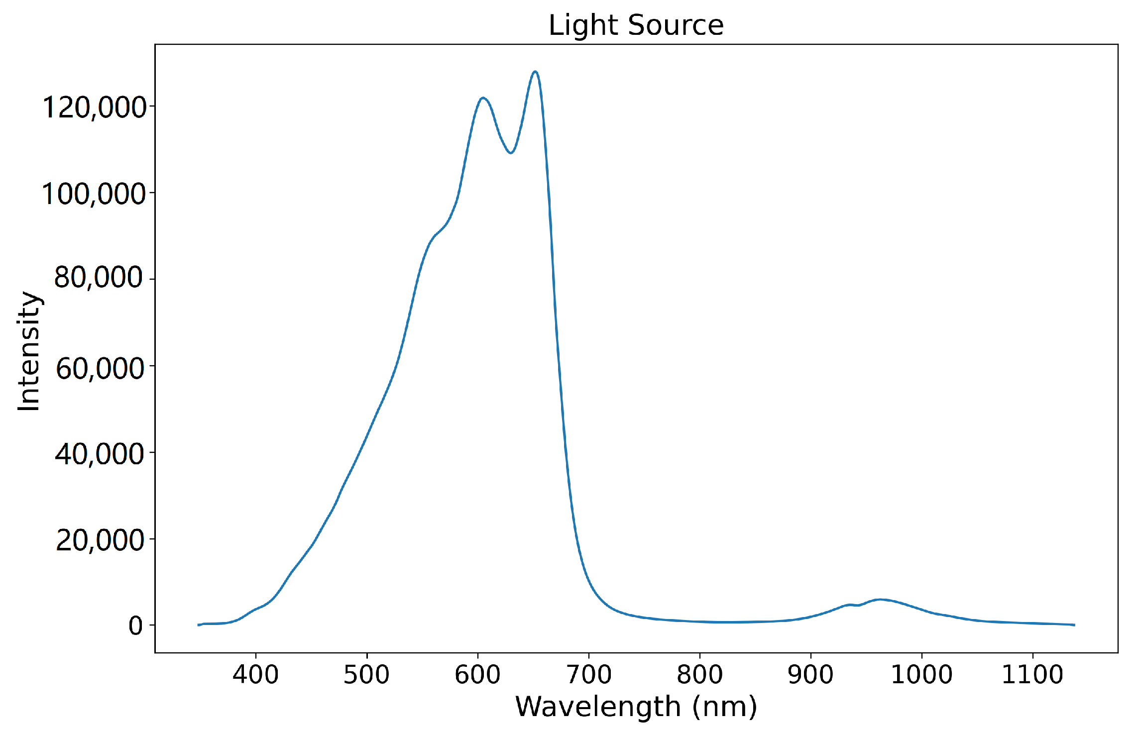
The focus of this study is on Yongquan tangerines, which are primarily grown in Yongquan, Linhai, Taizhou, and Zhejiang, China. A total of 150 tangerines were purchased from the same farmer in November 2022, with the requirement that the tangerines be of similar size and that no more than 20 tangerines be picked from the same tree, to ensure the diversity of the samples. During the experiment, some tangerines were damaged, so the number of valid samples is 118. The tangerines were gently wiped with a paper towel, numbered, and stored at room temperature (around 23 C). The 118 samples were measured in batches, and for each batch, the collection of spectra and the determination of quality parameters were completed on the same day. The spectra measurement system was set up consisting of the QE Pro spectrometer (Ocean Optics, Dunedin, FL, USA), two fibers, the Halogen light source (HLG-150W), and a personal computer. The spectral resolution of the QE Pro is 0.798 nm, and the integration time was set as 0.2 s. The dark noise correction and nonlinear correction were enabled in the OceanView software, and the average sliding width was set as 2, to reduce the effect of noises associated with the whole system. The wavelength is in the Vis–NIR range, specifically between 348.311 nm and 1137.377 nm, containing 1044 wavelengths. The transmittance spectra were acquired as depicted in Figure 1, where for each tangerine sample, the spectra of 12 locations were collected, including four around the equatorial position, four around the top area, and four around the bottom area. Therefore, a total of 118 × 12 measurements were conducted. The emission of the light source HLG-150W is depicted in Figure 2.
The raw spectra are converted to absorbance values according to Equation (1):
A = log 10 T = log 10 I I 0
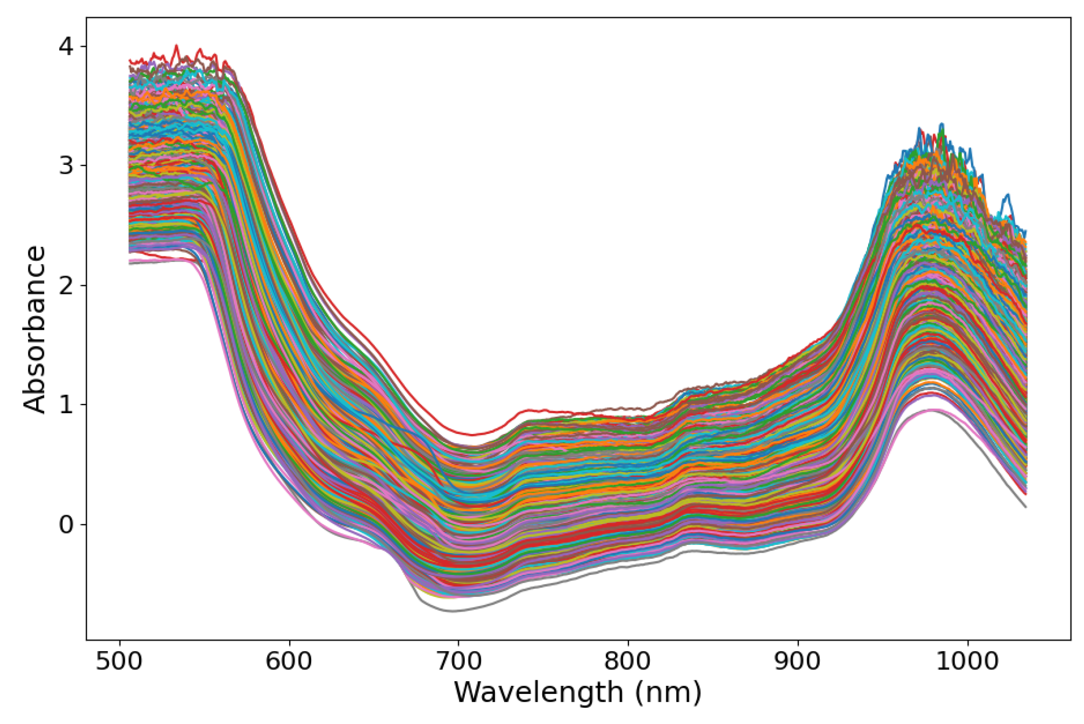
where I 0 represents the background spectra taken without the sample present, I represents the amount of light that reaches the detector, and consequently, and I / I 0 is the fraction of the incident light that penetrated the sample and detected [24]. The two ends of Vis–NIR spectra are eliminated where the signal-to-noise ratio is low and spectra between 550 nm and 1100 nm are retained, thus the shape of the spectra data is 118 samples, 12 locations, 701 wavelengths. The absorbance of 118 tangerines is depicted in Figure 3.

2.2. Internal Quality Attributes Assessment

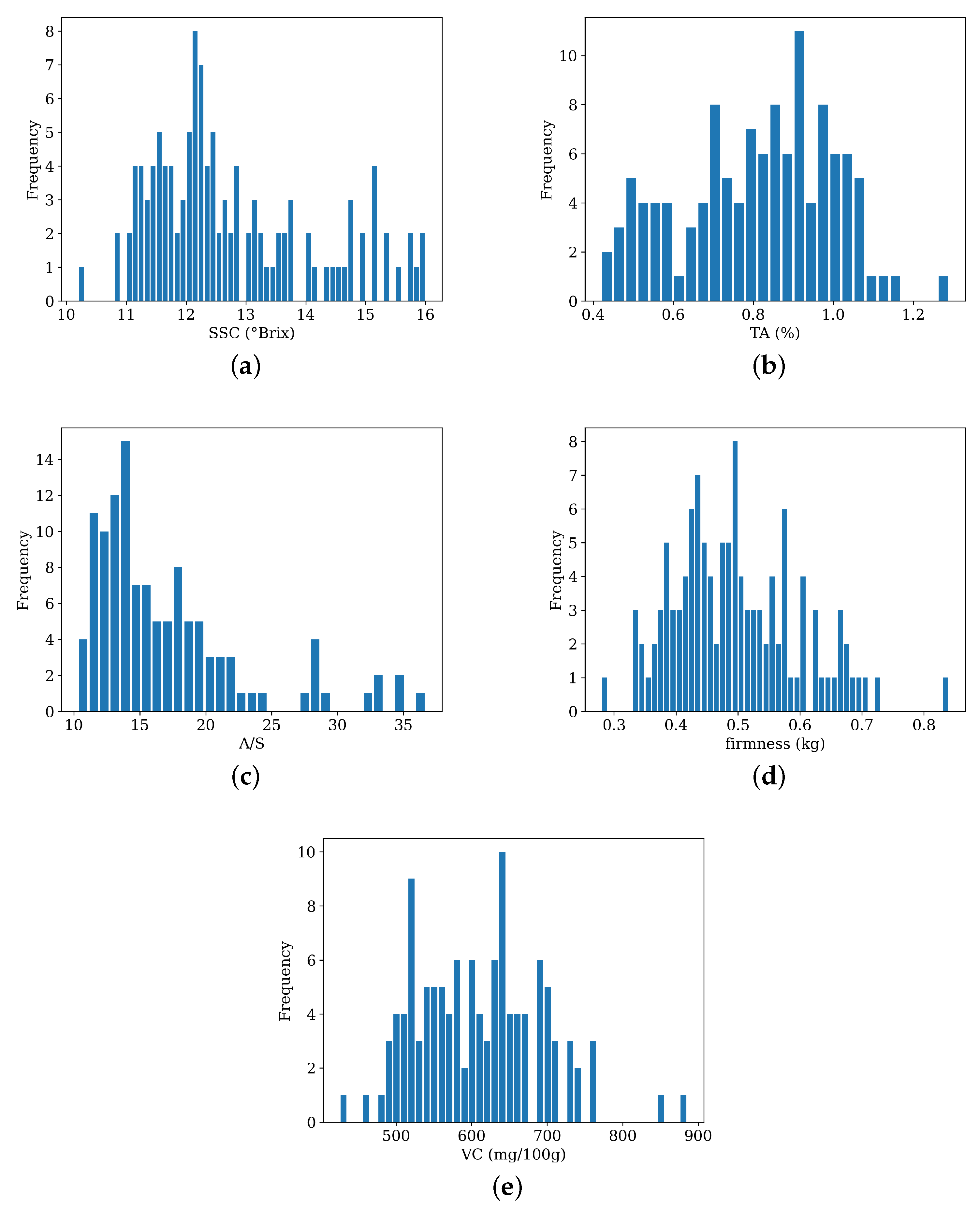
Destructive analysis of tangerines was performed at room temperature of approximately 23 C. The tangerine samples were peeled after spectra collection. First, to measure the firmness of tangerines, the probe of the GY-4 fruit firmness tester (HANDPI, Wenzhou, China) was inserted into the pulp of eight different parts of each tangerine and the mean value is taken as the final firmness of the tangerine. Next, each tangerine was squeezed individually in an automatic squeezer. The juice was then filtered and the total soluble solid content (SSC), total acidity (TA), and acid–sugar ratio (A/S) were measured using a digital refractometer (Atago Model PAL-BX|ACID F5, Tokyo, Japan). The determination of Vitamin C (VC) was conducted using the 2,6-dichlorophenolindophenol (DCPIP) titration method. This method relies on the oxidation-reduction titration of the acidic extract of the sample containing L(+)-ascorbic acid with a standard solution of 2,6-dichlorophenolindophenol. The reaction between ascorbic acid and DCPIP results in a color change, allowing for the quantitative determination of Vitamin C content (mg/100 g) [25]. The statistical information of the tangerine samples is listed in Table 1 and the histograms for the five quality parameters are shown in Figure 4.

2.3. Preprocessing Methods

Data preprocessing methods are essential to separate signal from noise and improve the signal-to-noise ratio in Vis–NIR spectra. The multiplicative scatter correction (MSC) method was introduced by Martens et al. [26], which is one of the most widely applied NIR preprocessing techniques. The primary objective of MSC is to mitigate spectral discrepancies associated with varying scattering levels present in the acquired spectral data, enhancing the correlation between spectral data and the target variables. By fitting a first-order function between the recorded spectra x r a w and a reference standard x r e f , the MSC technique can eliminate additive and multiplicative linear imperfections:
x r a w = b 0 + b 1 · x r e f + e
where b 0 represents the additive part and b 1 the multiplicative part. Generally, the reference spectrum employed is the average spectrum obtained from the sample set. The scatter-corrected spectra x c o r r is thus calculated as:
x c o r r = x r a w b 0 b 1
To prevent the amplification of noise within imperfect data, Savitzky–Golay (SG) derivatization [27] was used in most cases. This method involves fitting a symmetric polynomial function around neighboring data for each point in the spectrum, generating a smoothed spectrum that retains its characteristic features. In this experiment, SG smoothing parameters were set to second-degree polynomial and 11 smoothing points, and the second-order derivative was computed. StandardScaler (SS) is a preprocessing technique commonly used in machine-learning and neural-network applications. SS transforms the input data so that it has zero mean and unit variance. This is carried out by subtracting the mean of each feature and dividing it by its standard deviation.
The most suitable preprocessing methods in this study are performed in this order: Savitzky–Golay 2nd-derivatization (SG), multiplicative scatter correction (MSC), and standard scaling (SS). Through preprocessing, the impact of noise disturbances can be effectively reduced.

3. Neural Networks

To demonstrate the superiority of the proposed algorithm, which combines GCN, 2D-CNN, and Bi-LSTM with attention mechanism, it is compared with two other deep-learning networks, DeepSpectra2D and CNN-AT.

3.1. DeepSpectra2D

DeepSpectra2D is based on the DeepSpectra [16] network, with appropriate modifications and improvements made to better suit the tasks and the characteristics of the input data in this study. The hyperparameters of this network were set to the best combination that was tried via experiments. The structure of DeepSpectra2D for tangerine regression is depicted in Figure 5.
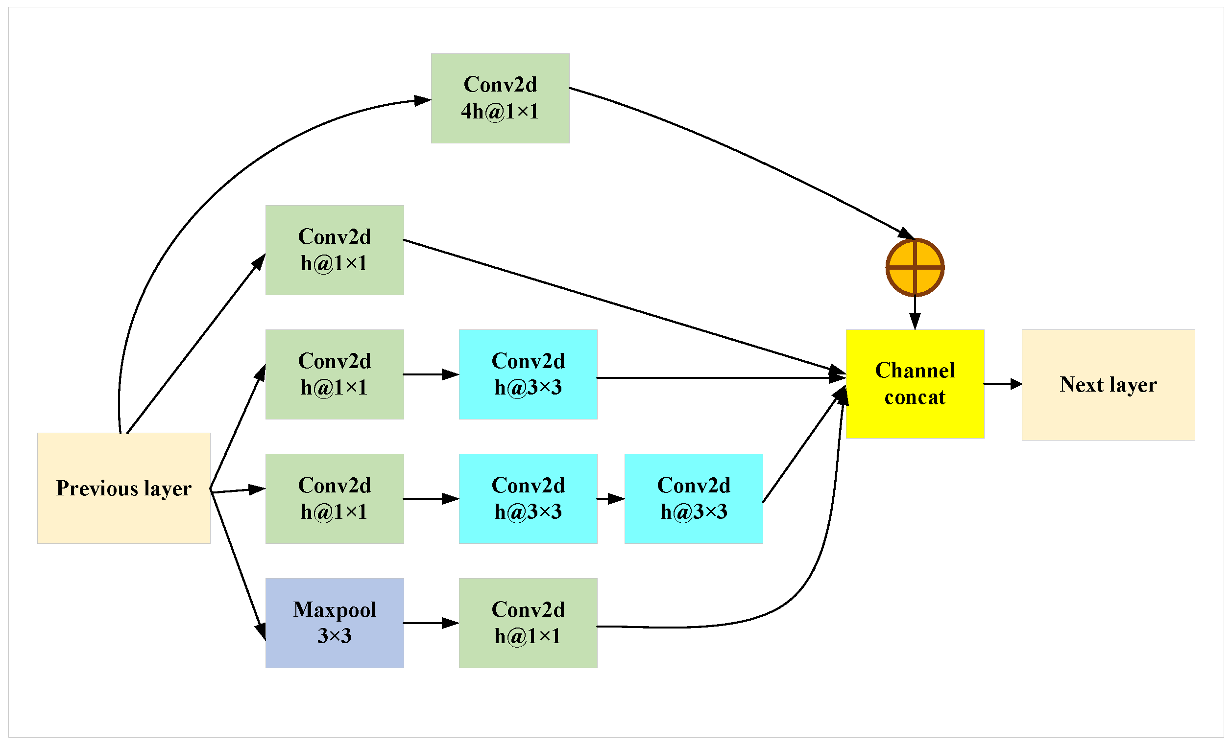
The Inception modules (InceptionA and InceptionB) incorporate multiple parallel convolutional pathways with different kernel sizes (1 × 1, 3 × 3, 5 × 5) to capture features at different scales and enrich the representation. The framework of the Inception module is shown in Figure 6.
In contrast to the inception module in [16], here, the 5 × 5 kernel is replaced by two layers of 3 × 3 kernel, which is better and was proposed in InceptionV2 [28]. The short-cut part was added, which is an idea proposed in the Residual Network [29] and widely used in deep learning. In DeepSpectra2D, each Conv2d layer is followed by max pooling to downsample the feature maps, reducing dimensions while preserving important features. The output from the InceptionB is flattened and fed into a fully connected layer to generate the final regression results. DeepSpectra2D utilizes multiple two-dimensional CNN layers and inserts Inception modules to hierarchically extract features from the spectra. This enables the network to learn complex relationships and capture both local and global patterns.

3.2. CNN-AT

CNN-AT is the combination of three blocks of hierarchical CNNs and an attention mechanism followed by a multi-layer perceptron (MLP). The flowchart of CNN-AT is shown in Figure 7.
CNN-AT consists of three CNN blocks (CONV1, CONV2, and CONV3) with diverse kernel sizes and different numbers of filters. Specifically, Conv2d in CONV1 possesses 8 filters with kernel size 1 × 25 , Conv2d in CONV2 has 16 filters with kernel size 1 × 15 and Conv2d in CONV3 contains 32 filters with kernel size 1 × 11 . Other compositions are the same in the three blocks: each Conv2d layer is followed by instance normalization (IN), parametric rectified linear unit activation (PReLU) [30], dropout, and max-pooling operations. The CNN-AT network incorporates an attention mechanism after the CNN blocks to selectively attend to specific parts of the input features. The output of the attention mechanism is then flattened and fed into MLP for further feature extraction and regression prediction. The MLP includes two fully connected layers (hidden size = 128), IN, PReLU, and a dropout rate of 0.2.

3.3. GCNN-LSTM-AT Network

This paper proposes an improved deep network called GCNN-LSTM-AT, which combines two-dimensional CNNs and LSTM, augmented by graph features and attention mechanism. The overall architecture is shown in Figure 8.

3.3.1. Graph Convolutional Network (GCN)

The application of GCN allows the model to capture the graph structure in the input data [31]. By leveraging the connections between nodes in the input data, GCN can capture the interactions and dependencies among nodes. This is particularly beneficial in dealing with data that exhibits complex correlations. The 12 locations on each tangerine have their own contextual information to some extent, while also being interdependent. To extract the relations between the 12 spectra, GCN processes the input data by generating graph-based features before putting it into the two-dimensional CNNs. The GCN is a layer-to-layer propagation, which is computed as:
H l + 1 = σ D ^ 1 2 A ^ D ^ 1 2 H l W l
where σ denotes the activation function (e.g., ReLU), W l is the trainable weights, H l is the matrix activation in layer l and H 0 = X . A ^ = A + I , A refers to the adjacency matrix, I is the identity matrix and D ^ i i = j A ^ i j .
The given input X R N × D represents N nodes with D features. The adjacency matrix A is calculated in a weighted way using the k-nearest neighbors algorithm ( N = 12 , D = 701 , k = 3 ). In this study, a two-layer GCN was employed, which is computed as:
Z = f ( X , A ) = D ^ 1 2 A ^ D ^ 1 2 ReLU D ^ 1 2 A ^ D ^ 1 2 X W 0 W 1
The output feature vector Z is duplicated two times and concatenated with the original spectra X (which is duplicated three times), obtaining an augmented feature of shape (n, 60, 701). This information propagation mechanism enables the model to utilize global information for inference and prediction, rather than relying solely on local features of each node.

3.3.2. Feature Extraction with CNNs

The second block employs two-dimensional CNNs and receives augmented spectra features from GCN as input. Two convolution layers are applied, aiming to capture spatial dependencies within the concatenated spectral features. The first layer performs convolution with a kernel size of [5, 26] and a stride of 1. The second layer performs convolution with a kernel size of [3, 27] and a stride of 1. After each convolution layer, Instance Normalization normalizes the output feature maps across the channel dimension for each individual sample in the batch. The PReLU activation function is used after each instance normalization layer. To promote the generalization of the model, dropout is applied after each activation function. Max pooling is employed following the dropout layer to reduce feature dimensionality and extract dominant features from the data. The CNN block allows the network to learn spatially local patterns and extract higher-level representations from the spectra data, output features of shape (n, 1, 13, 156). The specific choices of kernel sizes, activation functions, and regularization parameters have been determined through experimentation to achieve the desired balance between model complexity and generalization performance.

3.3.3. Sequential Modeling with LSTM

In the third block, a two-layer bidirectional long short-term memory (Bi-LSTM) is applied to capture features based on wavelength sequences. The Bi-LSTM processes the input both forward and backward in sequence steps to capture context from both directions. For each element in the input sequence, each LSTM layer computes the following functions:
i t = σ W i i x t + b i i + W h i h t 1 + b h i
f t = σ W i f x t + b i f + W h f h t 1 + b h f
g t = tanh W i g x t + b i g + W h g h t 1 + b h g
o t = σ W i o x t + b i o + W h o h t 1 + b h o
c t = f t c t 1 + i t g t
h t = o t tanh c t
where x t , h t , and c t are the input, hidden state, and cell state at step t, respectively. f t , g t , o t are the forget, cell, and output gates, respectively. σ is the sigmoid function and ⊙ is the Hadamard product. In a multi-layer LSTM, the input x t l of the lth layer ( l 2 ) is the hidden state h t l 1 of the previous layer.
In a Bi-LSTM, the hidden states of the forward and backward LSTM are concatenated at each time step, creating a more expressive feature representation. This allows the model to capture and utilize information from both directions, leading to a better representation and understanding of the sequence. In the implementation of this block, the input tensor is squeezed into the shape of (n, 13, 156). Each Bi-LSTM layer has 64 hidden units, so the output shape is (n, 13, 128).

3.3.4. Attention Mechanism

Bi-LSTM outputs a series of hidden states at each time step for downstream tasks. The self-attention mechanism [20] is employed to assign different weights to the hidden states of all time steps in the Bi-LSTM output, aiming to extract more informative feature representations for the regression task.
For each time step, given the output of Bi-LSTM with the shape of (n, 13, 128), the features are split into two parts—the forward hidden states h f ( t ) and the backward hidden states h b ( t ) —with the same shape of (n, 13, 64). Features after self-attention are given by:
s = t T α ( t ) h f ( t )
where a ( t ) is the weight learned by attention to measure the importance of the backward hidden states and is calculated as:
α ( t ) = s o f t m a x ( v ( t ) )
v ( t ) = W × h b ( t ) + b
where W and b are learnable weights and bias.
Finally, the output of the attention mechanism is flattened and passed through a fully connected layer to produce the regression results. The fully connected layer maps the learned features to the desired output dimension, enabling the network to predict continuous values for regression tasks.

4. Results and Discussion

4.1. Model Evaluation

The performance of each model is evaluated by root mean squared error of cross-validation (RMSECV), coefficient of determination ( R 2 ), and mean absolute error (MAE). Their calculations are shown in Equations (15)–(17).
R M S E C V = n = 1 N y n y ^ n 2 N
R 2 = n = 1 N y ^ n y n 2 n = 1 N y ¯ y n 2
M A E = n = 1 N y n y ^ n N
where y n and y ^ n are true target values and predicted values, respectively. N is the number of samples and y ¯ is the arithmetic mean of y n . The aforementioned metrics are averaged after obtaining 10-fold cross-validation results.
All the algorithms are implemented on the Python platform using PyTorch and Scikit-learn library, which are run on Windows 10 with 32 GB of RAM, and an Nvidia GeForce RTX 2060 (12 GB) (Nvidia, Santa Clara, CA, USA).

4.2. Comparison with Conventional Machine-Learning Approaches and Two Deep Networks

To compare the proposed GCNN-LSTM-AT model with conventional machine-learning approaches, three popular linear and nonlinear methods are taken into consideration, namely Moving Window Partial Least Squares (MWPLS) [32], Random Forest Regression (RF), and Support Vector Regression (SVR). Parameters of these methods have been optimized. For the SVR approach, GridSearch is employed to choose the kernel function from [‘linear’, ‘poly’, ‘rbf’], the penalty parameter from [0.001, 0.01, 0.1, 1, 10, 100, 1000], and the poly degree from [2, 3, 5]. MWPLS incorporates the concept of moving windows analysis to capture local variations, which performs better than PLS. RF combines the strength of decision trees and ensemble learning. GridSearch is employed in RF to select the number of estimators from range (50, 300) in step 50, the maximum depth from [5, 10, 20], the minimum split of sample from [2, 4, 8] and the minimum leaf of sample from [1, 2, 4]. The compared two other deep networks—DeepSpectra2D and CNN-AT—are already introduced in detail in the above section. The overall results for predicting the five target qualities of tangerines using all six algorithms are listed in Table 2. The results in the table are sorted in descending order by the value of R 2 .
As can be concluded from the table, the proposed GCNN-LSTM-AT model outperforms the three conventional approaches and two other deep networks in almost all scenarios in this study, except that it is a little worse than DeepSpectra2D for predicting VC. For the prediction of SSC ( Brix), various algorithms demonstrate good performance. Among them, GCN-LSTM-AT achieves the best performance with the lowest RMSECV (0.1430 Brix), the highest R 2 (0.9885), and the smallest MAE (0.1197 Brix). CNN-AT obtains the second-best performance, which achieves R 2 0.9300, RMSECV 0.4413 Brix and MAE 0.4034 Brix). The worst results are obtained by RF. In the evaluation of TA (%) prediction, GCN-LSTM-AT demonstrates better performance than other methods with R 2 0.8075, RMSECV 0.0868% and MAE 0.0721%. RF based on GridSearch provides the second-best prediction ( R 2 is 0.7085, RMSECV is 0.106826%, and MAE is 0.09584% in optimal case). When predicting A/S, R 2 can be improved to 0.901365 by GCN-LSTM-AT, which is much higher than the second-best method of 0.669026 based on the CNN-AT. The RMSECV of GCN-LSTM-AT is reduced to 1.998381, which is 44.81% less compared to CNN-AT. Regarding the target firmness (kg), GCN-LSTM-AT outperforms the other methods in terms of the highest R 2 (0.9472), while DeepSpectra2D obtains a lower R 2 (0.8203). The worst results are from SVR with R 2 0.19752. Results from the VC (mg/100 g) prediction reveal the good performance of DeepSpectra2D. It achieves the lowest RMSECV of 28.9411 (mg/100 g) and the highest R 2 of 0.74686 while GCN-LSTM-AT obtains the smallest MAE of 23.131868 (mg/100 g) and a slightly lower R 2 of 0.7386 than DeepSpectra2D, and the RMSECV is 29.410427 (mg/100 g). Despite being just slightly inferior to DeepSpectra2D in the prediction of VC, GCN-LSTM-AT shows significant improvement compared to other algorithms and performs consistently satisfactorily.
One notable observation from results of traditional algorithms is that the optimal hyperparameters for RF and SVR varied across different prediction targets. This finding underscores the sensitivity of RF and SVR to specific characteristics of the prediction task at hand. For MWPLS, the choice of window size is critical and can impact the model performance. Determining the optimal window size requires careful consideration and experimentation. Also, MWPLS involves performing PLS regression multiple times within different windows, which increases the computational complexity. In contrast, our proposed algorithm GCNN-LSTM-AT demonstrates a distinct advantage in this regard. Unlike RF, which requires meticulous tuning of hyperparameters for each prediction target, our algorithm exhibits robustness and adaptability, consistently showing competitive performance across a range of prediction tasks.
In comparison to the two deep networks, GCNN-LSTM-AT demonstrates stable and satisfactory performance in all five prediction tasks. DeepSpectra2D and CNN-AT have shown good performance in certain tasks, but they achieve unsatisfactory results at times. It indicates that GCNN-LSTM-AT can adapt well to various task characteristics and has better generalization ability. GCNN-LSTM-AT combines the advantage of GCN, diverse CNN kernels, Bi-LSTM, and the attention mechanism. GCN propagates node features and aggregates graph information, CNN is used to extract local features in the spatial dimension, while Bi-LSTM models the spectral sequential characteristics. This hierarchical representation learning enables the model to capture various relationships and patterns, enhancing the model’s expressive ability.
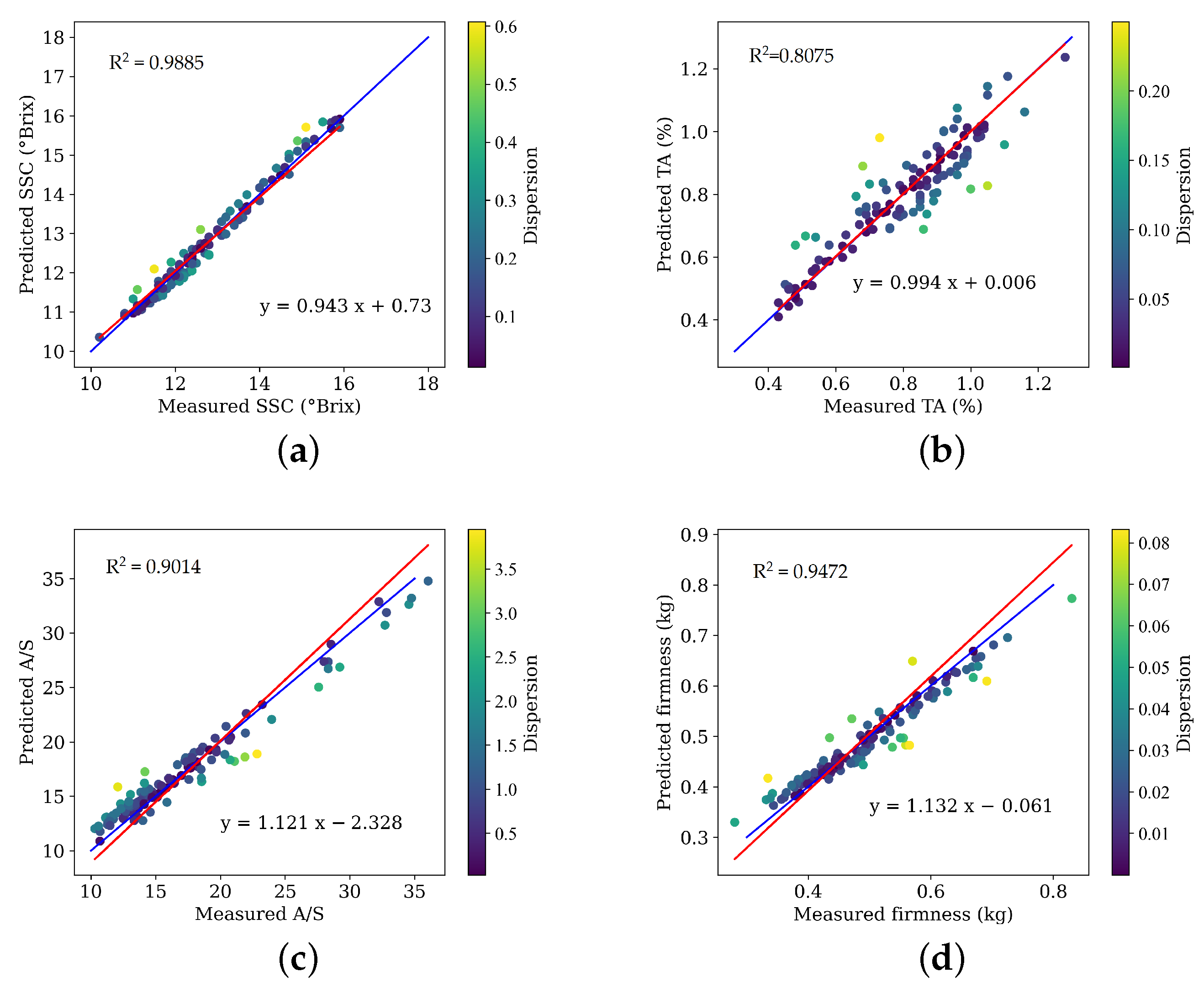
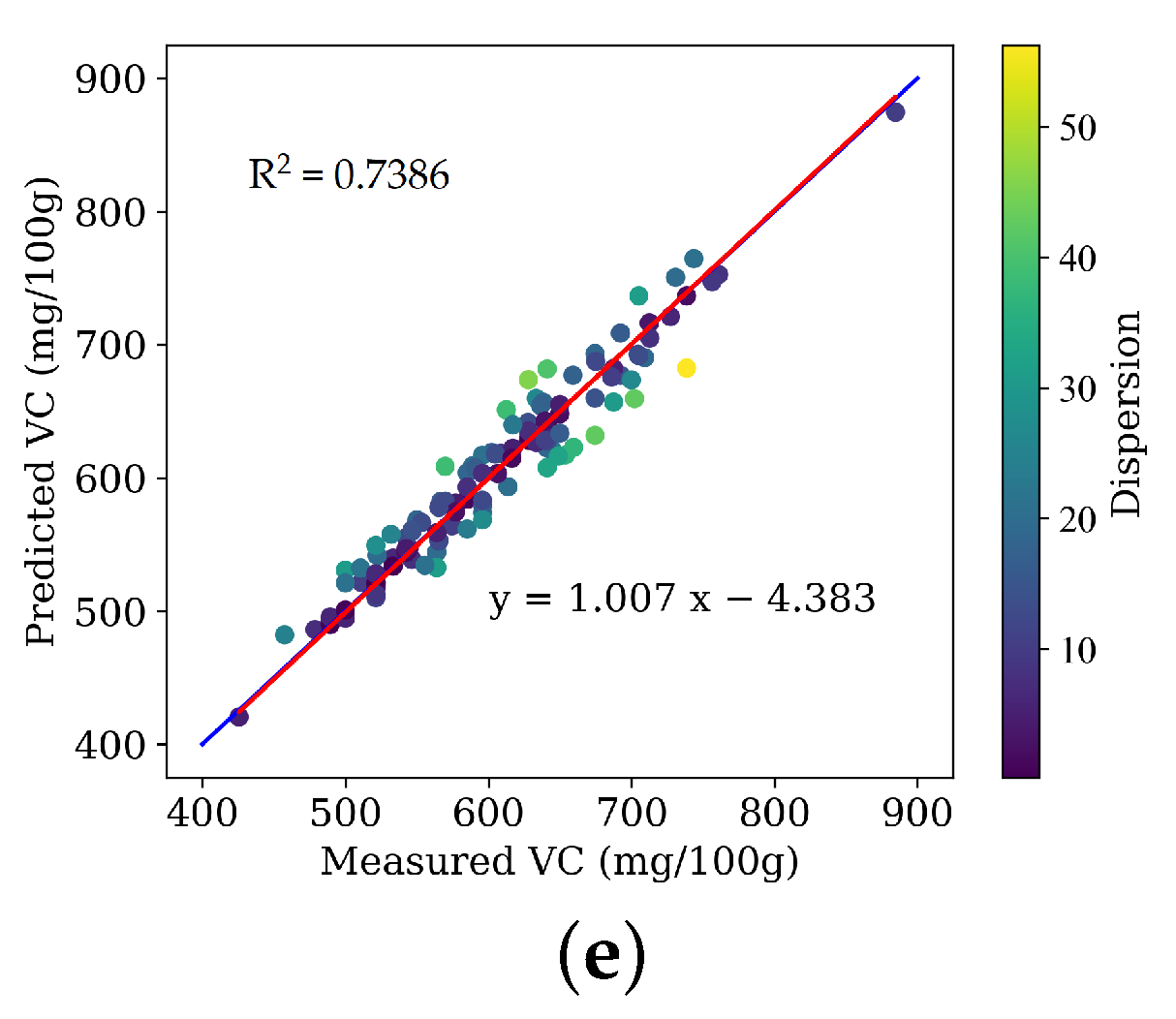
Figure 9 depicts the predictive performance of the proposed GCNN-LSTM-AT algorithm for five quality parameters on all tangerines. The x-axis of each dot in the figures is the actual measured value, and the y-axis is the predicted value of the model. The dispersion of each point is demonstrated by the color bar, where dark blue represents a small dispersion and yellow represents a larger dispersion. The red line is the fitting line between the predicted values and the true values, the slope and intercept of which are labeled in the figures. The blue line is the reference line, which is y = x . From the five scatter plots, it can be seen that the proposed algorithm can predict the SSC, TA, A/S, firmness, and VC of tangerines with relatively high accuracy, indicating good applicability. Among them, the prediction performance for SSC is the best, with the smallest prediction error and the highest degree of fit. Although the R 2 of VC is only 0.7386, the fitting line in Figure 9e looks good. This is partly because the range of VC and the interval value of axes are relatively large. In addition, existing literature has pointed out that R 2 can measure the goodness of fit in regression models, but it cannot compare the accuracy of model predictions, so R 2 , RMSECV and MAE should be taken into account in a combined way [33,34,35]. In Figure 9b, the red fitting line almost coincides with the blue reference line, but the degree of dispersion between each point and the fitting line is notable. The fitting lines between the predicted values and the true values plotted in the figures are employed as a reference to visually show the prediction performance of the model. The specific slope and intercept values of the fitting lines are independent for different datasets and it is not comparable when predicting different targets.

5. Conclusions

In this study, we propose a novel GCNN-LSTM-AT network for the prediction of five quality parameters of tangerines using Vis–NIR spectroscopy. GCNN-LSTM-AT combines two-dimensional CNN and Bi-LSTM networks, aided by graph features and the attention mechanism, to effectively capture the spatial and wavelength sequential dependencies in spectra data. Experimental results demonstrate the superior performance of the proposed network compared to other traditional algorithms and two deep neural networks, DeepSpectra2D and CNN-AT. The GCNN-LSTM-AT network achieves the lowest RMSECV, highest R 2 , and smallest MAE prediction of SSC, TA, A/S, and firmness. Although it is slightly inferior to DeepSpectra2D in the evaluation of VC, GCNN-LSTM-AT obtains more outstanding performance overall and shows better generalization ability than the other algorithms for diverse prediction targets. These results suggest that our method has strong potential for application on packing lines, allowing for the assessment of up to 10 fruits per second, quickly and accurately. However, in the future, more work ought to be conducted on online systems, which are specific to post-harvest applications, in which fruit of different qualities need to be graded and packed according to sorting categories. Future work should consider a dedicated design for an online application including a mechanical subsystem, communication subsystem, and spectral detection subsystem that prioritizes easy maintenance, easy modification for different products, and high working efficiency. For online systems, obtaining accurate spectral data from samples is difficult due to the complex working conditions and external parameters. It is, therefore, necessary to consider these parameters when establishing the whole system.

Author Contributions

Conceptualization, S.H.; methodology, Y.W.; software, Y.W.; validation, Y.W.; formal analysis, Y.W.; investigation, X.Z.; resources, Q.H.; data curation, Y.W. and Y.Z.; writing—original draft preparation, Y.W.; writing—review and editing, Y.W., J.E. and S.H.; visualization, Y.W.; supervision, S.H.; project administration, S.H.; funding acquisition, S.H. All authors have read and agreed to the published version of the manuscript.

Funding

This research was funded by “Pioneer” and “Leading Goose” R&D Program of Zhejiang Province (grant number 2023C03135), Ningbo Science and Technology Project under Grant 2021Z076 and National Natural Science Foundation of China (11621101).

Institutional Review Board Statement

Not applicable.

Informed Consent Statement

Not applicable.

Data Availability Statement

Not applicable.

Acknowledgments

The authors are grateful to Tengfei Ma of Zhejiang University for valuable discussions.

Conflicts of Interest

The authors declare no conflict of interest.

References

  1. Luo, J.; Lin, Z.; Xing, Y.; Forsberg, E.; Wu, C.; Zhu, X.; Guo, T.; Gaoxuan, W.; Bian, B.; Wu, D.; et al. Portable 4D Snapshot Hyperspectral Imager for Fastspectral and Surface Morphology Measurements. Prog. Electromagn. Res. 2022, 173, 25–36. [Google Scholar] [CrossRef]
  2. Nicolaï, B.; Beullens, K.; Bobelyn, E.; Peirs, A.; Saeys, W.; Theron, K.; Lammertyn, J. Nondestructive measurement of fruit and vegetable quality by means of NIR spectroscopy: A review. Postharvest Biol. Technol. 2007, 46, 99–118. [Google Scholar] [CrossRef]
  3. Ncama, K.; Opara, U.L.; Tesfay, S.Z.; Fawole, O.A.; Magwaza, L.S. Application of Vis/NIR spectroscopy for predicting sweetness and flavour parameters of ‘Valencia’ orange (Citrus sinensis) and ‘Star Ruby’ grapefruit (Citrus × paradisi Macfad). J. Food Eng. 2017, 193, 86–94. [Google Scholar] [CrossRef]
  4. Abbaspour-Gilandeh, Y.; Soltani Nazarloo, A. Non-Destructive Measurement of Quality Parameters of Apple Fruit by Using Visible/Near-Infrared Spectroscopy and Multivariate Regression Analysis. Sustainability 2022, 14, 14918. [Google Scholar] [CrossRef]
  5. Grabska, J.; Beć, K.; Ueno, N.; Huck, C. Analyzing the Quality Parameters of Apples by Spectroscopy from Vis/NIR to NIR Region: A Comprehensive Review. Foods 2023, 12, 1946. [Google Scholar] [CrossRef] [PubMed]
  6. Ribeiro, J.S.; Salva, T.d.J.G.; Silvarolla, M.B. Prediction of a wide range of compounds concentration in raw coffee beans using NIRS, PLS and variable selection. Food Control 2021, 125, 107967. [Google Scholar] [CrossRef]
  7. Xu, S.; Lu, B.; Baldea, M.; Edgar, T.F.; Nixon, M. An improved variable selection method for support vector regression in NIR spectral modeling. J. Process Control 2018, 67, 83–93. [Google Scholar] [CrossRef]
  8. Zhan, B.; Xiao, X.; Pan, F.; Luo, W.; Dong, W.; Tian, P.; Zhang, H. Determination of SSC and TA content of pear by Vis-NIR spectroscopy combined CARS and RF algorithm. Int. J. Wirel. Mob. Comput. 2021, 21, 41–51. [Google Scholar] [CrossRef]
  9. Sun, R.; Zhou, J.y.; Yu, D. Nondestructive prediction model of internal hardness attribute of fig fruit using NIR spectroscopy and RF. Multimed. Tools Appl. 2021, 80, 21579–21594. [Google Scholar] [CrossRef]
  10. Zhang, C.; Wu, W.; Zhou, L.; Cheng, H.; Ye, X.; He, Y. Developing deep learning based regression approaches for determination of chemical compositions in dry black goji berries (Lycium ruthenicum Murr.) using near-infrared hyperspectral imaging. Food Chem. 2020, 319, 126536. [Google Scholar] [CrossRef]
  11. Fukuhara, M.; Fujiwara, K.; Maruyama, Y.; Itoh, H. Feature visualization of Raman spectrum analysis with deep convolutional neural network. Anal. Chim. Acta 2019, 1087, 11–19. [Google Scholar] [CrossRef]
  12. Wei, X.; He, J.; Zheng, S.; Ye, D. Modeling for SSC and firmness detection of persimmon based on NIR hyperspectral imaging by sample partitioning and variables selection. Infrared Phys. Technol. 2020, 105, 103099. [Google Scholar] [CrossRef]
  13. Gong, D.; Ma, T.; Evans, J.; He, S. Deep Neural Networks for Image Super-Resolution in Optical Microscopy by Using Modified Hybrid Task Cascade U-Net. Prog. Electromagn. Res. 2021, 171, 185–199. [Google Scholar] [CrossRef]
  14. Shou, Y.; Yiming, F.; Chen, H.; Qian, H. Deep Learning Approach Based Optical Edge Detection Using Enz Layers (Invited). Prog. Electromagn. Res. 2022, 175, 81–89. [Google Scholar] [CrossRef]
  15. Zhang, X.; Yang, J.; Lin, T.; Ying, Y. Food and agro-product quality evaluation based on spectroscopy and deep learning: A review. Trends Food Sci. Technol. 2021, 112, 431–441. [Google Scholar] [CrossRef]
  16. Zhang, X.; Lin, T.; Xu, J.; Luo, X.; Ying, Y. DeepSpectra: An end-to-end deep learning approach for quantitative spectral analysis. Anal. Chim. Acta 2019, 1058, 48–57. [Google Scholar] [CrossRef]
  17. Hochreiter, S.; Schmidhuber, J. Long Short-Term Memory. Neural Comput. 1997, 9, 1735–1780. [Google Scholar] [CrossRef]
  18. Tan, A.; Wang, Y.; Zhao, Y.; Wang, B.; Li, X.; Wang, A.X. Near infrared spectroscopy quantification based on Bi-LSTM and transfer learning for new scenarios. Spectrochim. Acta Part A Mol. Biomol. Spectrosc. 2022, 283, 121759. [Google Scholar] [CrossRef]
  19. Chen, C.; Yang, B.; Si, R.; Chen, C.; Chen, F.; Gao, R.; Li, Y.; Tang, J.; Lv, X. Fast detection of cumin and fennel using NIR spectroscopy combined with deep learning algorithms. Optik 2021, 242, 167080. [Google Scholar] [CrossRef]
  20. Vaswani, A.; Shazeer, N.; Parmar, N.; Uszkoreit, J.; Jones, L.; Gomez, A.N.; Kaiser, L.; Polosukhin, I. Attention Is All You Need. arXiv 2017, arXiv:1706.03762. [Google Scholar]
  21. Ma, T.; Lyu, H.; Liu, J.; Xia, Y.; Qian, C.; Evans, J.; Xu, W.; Hu, J.; Hu, S.; He, S. Distinguishing bipolar depression from major depressive disorder using fnirs and deep neural network. Prog. Electromagn. Res. 2020, 169, 73–86. [Google Scholar] [CrossRef]
  22. Zheng, Z.; Liu, Y.; He, M.; Chen, D.; Sun, L.; Zhu, F. Effective band selection of hyperspectral image by an attention mechanism-based convolutional network. RSC Adv. 2022, 12, 8750–8759. [Google Scholar] [CrossRef]
  23. Yang, J.; Xu, J.; Zhang, X.; Wu, C.; Lin, T.; Ying, Y. Deep learning for vibrational spectral analysis: Recent progress and a practical guide. Anal. Chim. Acta 2019, 1081, 6–17. [Google Scholar] [CrossRef]
  24. Pasquini, C. Near Infrared Spectroscopy: Fundamentals, practical aspects and analytical applications. J. Braz. Chem. Soc. 2003, 14, 198–219. [Google Scholar] [CrossRef] [Green Version]
  25. Chang, S.; Ismail, A.; Daud, Z. Ascorbic Acid: Properties, Determination and Uses. In Encyclopedia of Food and Health; Caballero, B., Finglas, P.M., Toldrá, F., Eds.; Academic Press: Oxford, UK, 2016; pp. 275–284. [Google Scholar] [CrossRef]
  26. Geladi, P.; MacDougall, D.; Martens, H. Linearization and Scatter-Correction for Near-Infrared Reflectance Spectra of Meat. Appl. Spectrosc. 1985, 39, 491–500. [Google Scholar] [CrossRef]
  27. Savitzky, A.; Golay, M.J.E. Smoothing and Differentiation of Data by Simplified Least Squares Procedures. Anal. Chem. 1964, 36, 1627–1639. [Google Scholar] [CrossRef]
  28. Szegedy, C.; Vanhoucke, V.; Ioffe, S.; Shlens, J.; Wojna, Z. Rethinking the Inception Architecture for Computer Vision. In Proceedings of the 2016 IEEE Conference on Computer Vision and Pattern Recognition (CVPR), Las Vegas, NV, USA, 26 June–1 July 2016; pp. 2818–2826. [Google Scholar] [CrossRef] [Green Version]
  29. He, K.; Zhang, X.; Ren, S.; Sun, J. Deep Residual Learning for Image Recognition. In Proceedings of the 2016 IEEE Conference on Computer Vision and Pattern Recognition (CVPR), Las Vegas, NV, USA, 26 June–1 July 2016. [Google Scholar]
  30. Xu, B.; Wang, N.; Chen, T.; Li, M. Empirical Evaluation of Rectified Activations in Convolutional Network. arXiv 2015, arXiv:1505.00853. [Google Scholar]
  31. Kipf, T.N.; Welling, M. Semi-Supervised Classification with Graph Convolutional Networks. arXiv 2016, arXiv:1609.02907. [Google Scholar]
  32. Jiang, J.H.; Berry, R.J.; Siesler, H.W.; Ozaki, Y. Wavelength Interval Selection in Multicomponent Spectral Analysis by Moving Window Partial Least-Squares Regression with Applications to Mid-Infrared and Near-Infrared Spectroscopic Data. Anal. Chem. 2002, 74, 3555–3565. [Google Scholar] [CrossRef] [PubMed]
  33. Anderson-Sprecher, R. Model Comparisons and R2. Am. Stat. 1994, 48, 113–117. [Google Scholar] [CrossRef]
  34. Chicco, D.; Warrens, M.J.; Jurman, G. The coefficient of determination R-squared is more informative than SMAPE, MAE, MAPE, MSE and RMSE in regression analysis evaluation. PeerJ Comput. Sci. 2021, 7, e623. [Google Scholar] [CrossRef] [PubMed]
  35. Spiess, A.N.; Neumeyer, N. An evaluation of R2 as an inadequate measure for nonlinear models in pharmacological and biochemical research: A Monte Carlo approach. BMC Pharmacol. 2010, 10, 6. [Google Scholar] [CrossRef] [PubMed] [Green Version]
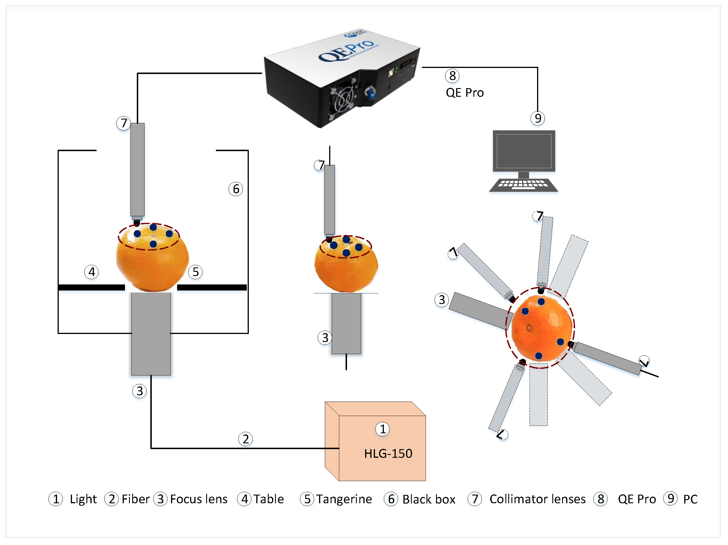
Figure 1. Schematic of the set-up for measuring the transmittance spectra of tangerines.
Applsci 13 08221 g001
Figure 2. The emission of the light source.
Applsci 13 08221 g002
Figure 3. The absorbance of 118 tangerines.
Applsci 13 08221 g003
Figure 4. Histograms for the five quality parameters of the 118 tangerines. (a) SSC, the bins are set at 0.1 Brix, (b) TA, the bins are set at 0.03%, (c) A/S, the bins are set at 0.8, (d) Firmness, the bins are set at 0.01 kg, (e) VC, the bins are set at 10 (mg/100 g).
Applsci 13 08221 g004
Figure 5. The structure of DeepSpectra2D.
Applsci 13 08221 g005
Figure 6. The framework of the Inception module.
Applsci 13 08221 g006
Figure 7. The framework of CNN-AT algorithm.
Applsci 13 08221 g007
Figure 8. The overall architecture of GCNN-LSTM-AT Network.
Applsci 13 08221 g008
Figure 9. Predictions of the proposed GCNN-LSTM-AT algorithm on the test set for five quality parameters of tangerines. (a) Soluble solid content (SSC) results. (b) Total acidity (TA) results. (c) Acid–sugar ratio (A/S) results. (d) Firmness results. (e) Vitamin C (VC) results.
Applsci 13 08221 g009aApplsci 13 08221 g009b
Table 1. The statistical information of the tangerine samples.
TargetMinMaxMeanSTDMeasurement Accuracy
SSC ( Brix)10.215.912.6971.3615±0.2%
TA (%)0.421.280.80370.1866±0.1%
A/S10.336.0516.9745.7591±0.3%
Firmness (kg)0.28020.83040.49580.1003±1%
VC (mg/100 g)425.5319884.6154608.977581.9140±2%
Table 2. Performance of six models on the five qualities of tangerines. The quality parameters are soluble solid content (SSC), total acidity (TA), acid–sugar ratio (A/S), firmness, and Vitamin C (VC).
TargetMethodRMSECV R 2 MAE
SSC ( Brix)GCNN-LSTM-AT0.1430190.9885460.119733
CNN-AT0.4413040.9300020.403427
MWPLS0.6306210.8570620.564087
DeepSpectra2D0.6339720.8555390.523082
SVR0.6350880.8550300.550726
RF0.6377210.8538260.545897
TA (%)GCNN-LSTM-AT0.0868170.8074870.072121
RF0.1068260.7085270.095840
CNN-AT0.112660.675820.080944
DeepSpectra2D0.1165520.6530380.097312
SVR0.1284810.5783780.115217
MWPLS0.1327570.5498450.110507
A/SGCNN-LSTM-AT1.9983810.9013651.600419
CNN-AT3.6210920.6690262.897637
RF3.660370.6618073.025368
SVR3.7875080.6379062.619833
DeepSpectra2D4.1720310.5606513.241931
MWPLS4.2345710.5473813.200423
Firmness (kg)GCNN-LSTM-AT0.0294080.9472060.020084
DeepSpectra2D0.0385970.8203010.027363
MWPLS0.0431780.7751090.035490
CNN-AT0.0489340.7111510.038188
RF0.0640570.5050320.052835
SVR0.0909670.197520.073538
VC (mg/100 g)DeepSpectra2D28.9410880.74685927.861427
GCNN-LSTM-AT29.4104270.73858323.131868
MWPLS35.4929730.61927125.987210
CNN-AT36.668470.59363530.667585
RF43.018740.44069831.808692
SVR45.5832220.37202733.289951
Disclaimer/Publisher’s Note: The statements, opinions and data contained in all publications are solely those of the individual author(s) and contributor(s) and not of MDPI and/or the editor(s). MDPI and/or the editor(s) disclaim responsibility for any injury to people or property resulting from any ideas, methods, instructions or products referred to in the content.