Opposite Normalized Trust-Region Reflective (ONTRR): A New Algorithm for Parameter Extraction of Single, Double and Triple Diode Solar Cell Models

Abstract

To accurately, efficiently and reliably extract the parameters of single, double and triple diode solar cell models, this paper proposes a randomly initialized opposite normalized trust-region reflective (ONTRR) algorithm. The novelty of ONTRR lies primarily in two amendments to the standard TRR search. (1) Random opposite initialization is added to decrease the initial point sensitivity of TRR and thus reduce the possibility of being trapped in local optima. (2) Min-max normalization is embedded to eliminate the negative effects arising from different magnitudes of model parameter values and thus drive the derivative-dependent TRR search in an efficient manner. The proposed ONTRR algorithm is evaluated and compared to other state-of-the-art algorithms using four benchmarked I–V datasets with two commonly used objective functions. To be objective and reproducible, the comparative experiments are carried out with default random seeds for 1000 independent runs instead of the 30, 50, or 100 runs used in most studies in the literature. The comparison results demonstrate that for all 12 of the test cases, the proposed ONTRR algorithm consistently achieves the highest accuracy with the least computational effort, and is often superior to the best-performing algorithms reported in the literature in terms of convergence speed, average accuracy and statistical stability.

1. Introduction

To improve the performance evaluation, fault detection and maximum energy harvesting of PV systems [1], one major focus of the research community is accurate modeling and efficient parameter extraction to closely represent the nonlinear I–V (current vs. voltage) characteristics of solar cells. Although various models have been developed to describe the electrical behavior of solar cells, only three equivalent circuit models are widely used [2]: the single diode model (SDM), the double diode model (DDM) and the triple diode model (TDM). Unfortunately, all three models are implicit nonlinear transcendental equations. This inherently implicit nature increases not only the difficulty of parameter extraction but also the complexity of PV system simulation, and thus calls for accurate, efficient and reliable methods to extract the model parameters from the measured I–V data of solar cells.

For solving the parameter extraction problem of SDM, DDM and TDM, various methods have been developed. These methods can be generally classified into analytical, deterministic, population-based stochastic search and hybrid algorithms. Analytical methods take several key points to generalize all measured I–V data, but the results are inaccurate. Deterministic algorithms, such as Newton–Raphson, pattern search and Nelder–Mead simplex search, are sensitive to initial values and thus prone to being trapped in local minima. Population-based stochastic algorithms, inspired by nature [3,4,5,6,7,8,9], biology [10,11,12,13,14,15,16], swarm [17] and evolution [18,19,20,21,22,23], usually require significant computational efforts to converge and depend strongly upon the proper tuning of control parameters, such as population size, the maximum number of function evaluations (MaxNFEs) or iterations, searching strategies and so on. Hybrid algorithms [24,25,26,27,28,29] combine the strengths of two or more different methods in an attempt to achieve better results. For example, the ABC-TRR [29] algorithm combined the global exploration capability of the artificial bee colony (ABC) algorithm and the local exploitation ability of trust-region reflective (TRR) search to extract the parameters of SDM and DDM. However, hybrid algorithms usually mean more control parameters that need to be carefully tuned. For instance, there are seven control parameters in the ABC-TRR [29] algorithm that need to be elaborately selected, and any improper choice could result in slow convergence and premature termination of iterations. Even though these algorithms provided accurate results, there is still room for improving their computational efficiency, convergence speed and reliability.

Motivated by the preceding discussion, this paper proposes an opposite-normalized trust-region reflective (ONTRR) algorithm aiming for accurate, efficient and reliable parameter extraction of SDM, DDM and TDM. Unlike the ABC-TRR [29] algorithm, the proposed ONTRR adopts random opposite initialization and min-max normalized processing to overcome the drawbacks of the standard TRR search. Initially, the proposed ONTRR generates a random point and its opposite point, and then selects the better of these two points as the initial point, which gives a higher chance of finding promising regions. In the iteration phase, the proposed ONTRR employs the unitary surrogate of model parameter values to calculate distances to the normalized boundary and truncate the unconstrained trial step to ensure a sufficient decrease of the derivative-dependent TRR search. Moreover, the proposed ONTRR omits the terminate tolerances of TRR search and adopts the only control parameter MaxNFEs to determine stop or not, which removes the burden of multi-parameter tuning and permits its use without prior knowledge about solar cell parameter extraction.

In general, the main novelties/contributions of this paper are as follows:

(1)

A randomly initialized, derivative-dependent algorithm ONTRR, which has only one control parameter, is developed for improving the parameter extraction of SDM, DDM and TDM.

(2)

Random opposite initialization is designed to decrease the initial point sensitivity of TRR and thus reduce its possibility of being trapped in local minima.

(3)

Min-max normalized processing is embedded into TRR to eliminate its sensitivity to the magnitude of model parameter values thereby improving convergence speed.

(4)

The proposed ONTRR algorithm is comprehensively tested on four benchmarked I–V datasets with two commonly used objective functions. To verify that the proposed ONTRR is reliable and not coincidental in a reproducible way, it is implemented with default random seeds for 1000 independent runs to compare with other state-of-the-art algorithms.

(5)

The comparison results demonstrate that the proposed ONTRR always exhibits the highest convergence speed to achieve the most accurate parameter values, and is more robust than the best-performing algorithms reported in the literature for solar cell parameter extraction.

2. Photovoltaic Modeling and Problem Formulation

2.1. Photovoltaic Modeling

As can be seen from Figure 1, a real solar cell is modeled by the equivalent circuits comprising of a photocurrent source I_ph, a lumped series resistance R_s, a lumped shunt resistance R_sh and one or several parallel diodes with different ideality factors. In Figure 1a, the diode D of SDM incorporates a nonphysical ideality factor n to account for the combined effect of more than one type of conduction mechanism within the actual solar cell. In Figure 1b, the first diode D₁ represents the conduction phenomena in quasi-neutral regions, while the second diode D₂ corresponds to the recombination in the space–charge region of the junction. In Figure 1c, the first two diodes D₁ and D₂ of TDM carry the same physical meaning as they did in DDM, while D₃ is exclusively designed to take the recombination losses in defect regions and grain boundaries into account with the ideality factor n₃. For a given irradiance and temperature, the I–V relationships in Figure 1a–c can be formulated by the SDM Equation (1), DDM Equation (2) and TDM Equation (3), respectively.

$$I=I_{ph}-I_0\left[\exp \left(\frac{V+I{R}_s}{n{V}_{th}}\right)-1\right]-\frac{V+I{R}_s}{R_{sh}}$$

(1)

$$I=I_{ph}-{\displaystyle \sum _{i=1}^2{I}_{0i}\left[\exp \left(\frac{V+I{R}_s}{n_i{V}_{th}}\right)-1\right]}-\frac{V+I{R}_s}{R_{sh}}$$

(2)

$$I=I_{ph}-{\displaystyle \sum _{i=1}^3{I}_{0i}\left[\exp \left(\frac{V+I{R}_s}{n_i{V}_{th}}\right)-1\right]}-\frac{V+I{R}_s}{R_{sh}}$$

(3)

where I, V, I_ph, I₀, I_0i, n, n_i, R_s and R_sh are the terminal current, terminal voltage, photocurrent, diode reverse saturation currents, diode ideality factors and series and shunt resistance, respectively. The thermal voltage V_th = kT/q, where the Boltzmann constant k = 1.3806503 × 10⁻²³ J/K, electronic charge q = 1.60217646 × 10⁻¹⁹ C and T is the absolute temperature in Kelvin.

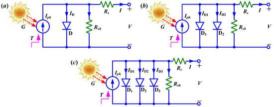
Figure 1. Equivalent circuit models of a real solar cell: (a) SDM, (b) DDM and (c) TDM.

It is easy to see from Equations (1)–(3) that there are five parameters X = [n, I_ph, I₀, R_s, R_sh] in SDM, seven parameters X = [n₁, n₂, I_ph, I₀₁, I₀₂, R_s, R_sh] in DDM and nine parameters X = [n₁, n₂, n₃, I_ph, I₀₁, I₀₂, I₀₃, R_s, R_sh] in TDM. Since SDM is a good compromise between simplicity and accuracy [30], it has been widely used to simulate the electrical behavior of solar modules with I_phm = I_phN_p, I_0m = I₀N_p, n_m = nN_s, R_sm = R_sN_s/N_p and R_shm = R_shN_s/N_p, where N_s stands for the number of cells in series while N_p represents the strings of cells connected in parallel.

2.2. Two Commonly Used Objective Functions

The main objective for solar cell parameter extraction is to find a set of parameter values to minimize the overall errors between the simulated current I_sim and measured current I under the same terminal voltage V. In this paper, the sum of square errors (SSE) is chosen as the objective function and the optimization goal is set to minimize Equation (4) with respect to the current error function f(X). For ease of comparison with the reported results, the root mean square error (RMSE) is also calculated with Equation (5). It is evident from Equations (4) and (5) that the smaller the SSE or RMSE values, the more accurate the parameter values extracted from the measured I–V data of the solar cells/modules.

$$F(X)=SSE(X)=\underset{X\in [\mathrm{LB},\mathrm{UB}]}{\min }{\displaystyle \sum _{j=1}^{N}f{(X)}^2}=\underset{X\in [\mathrm{LB},\mathrm{UB}]}{\min }{\displaystyle \sum _{j=1}^N{\left[I_{sim}(X)-I\right]}^2}$$

(4)

$$RMSE=\sqrt{F(X)/N}$$

(5)

where the model parameter vector X is constrained within a lower bound (LB) and an upper bound (UB) and N is the number of measured I–V data points. To simplify the calculation of I_sim, the most commonly used implicit exponential function (IEF) method expresses/replaces it with the measured current I. By the direct application of Equations (1)–(3), it can be formulated as:

$$I_{sim}(X)=I_{ph}-{\displaystyle \sum _{i=1}^{N_d}{I}_{0i}\left[\exp \left(\frac{V+I{R}_s}{n_i{V}_{th}}\right)-1\right]}-\frac{V+I{R}_s}{R_{sh}}$$

(6)

where N_d denotes the number of parallel diodes in Figure 1a–c and can be seen as a pointer mapping to SDM when N_d = 1, DDM when N_d = 2 and TDM when N_d = 3, respectively.

It is clear from Equation (6) that I_sim is characterized by the fact that the measured current I and voltage V appear simultaneously. This implicit expression increases the complexity and difficulty of parameter extraction, thereby making Equation (6) less accurate than the Lambert W function (LWF)-based approximate explicit expression [3,4]:

$$I_{sim}(X)=\frac{I_{ph}+{\displaystyle {\sum }_{i=1}^{N_d}{I}_{0i}}-V/R_{sh}}{1+R_s/R_{sh}}-\frac{V_{th}}{R_s}{\displaystyle \sum _{i=1}^{N_d}{n}_i{W}_0(S{U}_i)}$$

(7)

where W₀ is the principal branch of Lambert W function and

$$S{U}_i=\frac{I_{0i}{R}_s}{n_i{V}_{th}(1+R_s/R_{sh})}\exp \left[\frac{R_s{I}_{ph}+R_s{I}_{0i}+V}{n_i{V}_{th}(1+R_s/R_{sh})}\right]$$

(8)

3. Trust-Region Reflective (TRR) Search

3.1. Trust-Region Method

The trust-region method is a conceptually simple yet powerful and derivative-dependent algorithm for solving nonlinear least-squares problems in the form of Equation (9), which is a perfect match for the objective function Equation (4).

$$F(X)=\underset{X\in [\mathrm{LB},\mathrm{UB}]}{\min }\left[f_1{(X)}^2+f_2{(X)}^2+\cdots +f_N{(X)}^2\right]$$

(9)

The essential idea behind the trust-region method is to approximate F(X) with a simpler quadratic function q(s) in a small neighborhood N_t around the current point X. This neighborhood is the trust region, whose shape ideally is spherical rather than ellipsoidal. By minimizing the trust-region sub-problem: min{q(s), s∈N_t}, a trial step s of current point X can be obtained, which indicates the direction to reduce F(X). If F(X + s) < F(X), the current point X is updated to be X + s; otherwise, X remains unchanged while the trust region radius Δ is shrunk for the next iteration. Hence, the key steps of the trust-region method [31] are:

(1)

Solve the trust-region sub-problem Equation (10) for determining a trial step s.

$$\min \left\{q(s):‖Ds‖\le \Delta \right\}$$

(10)

(2)

Truncate the trial step s with Equation (11) to ensure X + αs is strictly feasible.

$$\alpha =\min (1,\theta \cdot mdis)$$

(11)

(3)

Compute the quadratic approximate function q(s) with Equation (12), where the first two terms of the Taylor expansion are employed to approximate [F(X + s) − F(X)]/2.

$$q(s)=g^{T}s+\frac{1}{2}{s}^T(H+C)s$$

(12)

(4)

Adjust the trust-region radius Δ according to Equation (13) and update the current point X to be X + s if F(X + s) < F(X).

$$\rho =\frac{0.5[F(X+s)-F(X)]+0.5s^{T}Cs}{q(s)}$$

(13)

where ‖.‖ is the Euclidean 2-norm and D is the diagonal affine scaling matrix defined by Equation (14), which is used to prevent s directly toward a boundary point. α is the step size toward the boundary along s, θ is defined by Equation (15) representing the correction of Δ and implies a potential step-back to ensure Δ is strictly feasible, while mdis is defined by Equation (16) and denotes the min-max breakpoint distances to the boundary. g is the gradient of error function f(X) and superscript ^T denotes the transpose operation. H is the Hessian matrix and can be approximated with the symmetric matrix of Equation (17). C is the affine scaling matrix defined by Equation (18). ρ measures the agreement between F(X) and its quadratic approximation q(s). Since F(X) is calculated by Equation (9), to match with q(s) in Equation (12), the coefficient of 0.5 in Equation (13) is necessary while the term of $0.5s^{T}Cs$ is a natural extension to the bound-constrained problem [31]. As for how to update Δ according to ρ, the empirical threshold values are formulated by Equation (19).

$$D=\mathrm{diag}(|v{|}^{-0.5})$$

(14)

$$\theta =\max (0.95,1-||v\cdot g|{|}_{\infty })$$

(15)

$$mdis=\min \left[\max \left(\frac{UB-X}{s},\frac{LB-X}{s}\right)\right]$$

(16)

$$H=J^{T}J$$

(17)

$$C=D\mathrm{diag}(g)J_{v}D$$

(18)

$$\Delta =\left\{\begin{array}{l}2\Delta ,\mathrm{if}\rho \ge 0.75\mathrm{and}\left|\right|Ds\left|\right|\ge 0.9\Delta \\ \Delta ,\mathrm{if}0.25<\rho <0.75\\ \min (\Delta /4,|\left|Ds\right||/4),\mathrm{if}\rho \le 0.25\end{array}\right.$$

(19)

where v denotes the distances to the boundary and can be computed by Equation (20). J denotes the Jacobian matrix estimated usually by the dense forward finite differences of error function f(X). J_v is a diagonal matrix corresponding to the Jacobian of |v|, with all diagonal components of J_v equal to 0 or ±1. If all the components of LB and UB are finite, J_v = diag(sign(g)). In particular, if v(i) = 0, the ith diagonal component of J_v equals 1.

$$\begin{array}{l}\mathrm{for}i=1\mathrm{to}\dim \mathrm{do}\\ \begin{array}{cc}\mathrm{if}g(i)<0\mathrm{and}\mathrm{UB}(i)<+\infty ,& v(i)=X(i)-\mathrm{UB}(i)\\ \mathrm{if}g(i)\ge 0\mathrm{and}\mathrm{LB}(i)>-\infty ,& v(i)=X(i)-\mathrm{LB}(i)\\ \mathrm{if}g(i)<0\mathrm{and}\mathrm{UB}(i)=+\infty ,& v(i)=-1\\ \mathrm{if}g(i)\ge 0\mathrm{and}\mathrm{LB}(i)=-\infty ,& v(i)=1\end{array}\end{array}$$

(20)

It should be noted that Equation (10) is defined to include the bound constraint, which was handled by adjusting Δ with 2-norm Euclidean distance constraints and the truncation effect in Equation (11) to satisfy strict feasibility. Consider the effect of D in C as a component of v approaches zero, by applying the affine scaling transformation $\widehat{X}=DX$ [32] to handle constraints implicitly, the bound-constrained problem Equation (9) can be reduced into an unconstrained problem. Therefore, X can be improved by solving the trust-region sub-problem Equation (21) and then transforming back to the original space.

$$\min \left\{\widehat{q}(\widehat{s})={\widehat{g}}^T\widehat{s}+\frac{1}{2}{\widehat{s}}^T\widehat{M}\widehat{s}:‖\widehat{s}‖\le \Delta \right\}$$

(21)

where

$$\widehat{M}=DHD+C$$

(22)

$$D=\mathrm{diag}(|v{|}^{0.5})$$

(23)

$$C=\mathrm{diag}(g)\mathrm{diag}\left(\mathrm{sign}\right(g\left)\right)$$

(24)

$$\widehat{g}=Dg$$

(25)

$$s=D\widehat{s}$$

(26)

3.2. Subspace Approach Solving Trust-Region Sub-Problem

Although accurate algorithms exist to solve Equation (21), they usually involve the computation of all eigenvalues of H and a Newton process for the secular equation (27). To circumvent costly solving Equation (27) in the full-space of dim variables and be beneficial for large-scale problems, an approximate subspace trust-region interior reflective algorithm [32] was proposed to restrict the full-space sub-problem to a 2-D subspace S. Once S is determined, it is trivial to solve the subspace sub-problem Equation (28) since it is just two-dimensional.

$$\frac{1}{\Delta }-\frac{1}{\left|\right|s\left|\right|}=0$$

(27)

$$\min \left\{\widehat{q}(\widehat{s}):‖\widehat{s}‖\le \Delta ,D\widehat{s}\in S\right\}$$

(28)

The 2-D subspace S is formed as the linear space spanned by ${\widehat{s}}_1$ and ${\widehat{s}}_2$, where ${\widehat{s}}_1$ is the gradient direction $\widehat{g}$, and ${\widehat{s}}_2$ is the output of a preconditioned conjugate gradient (PCG) process, either an inexact Newton direction defined by Equation (29) or a direction of negative curvature satisfying Equation (30).

$$\widehat{M}{\widehat{s}}_2=-\widehat{g}$$

(29)

$${\widehat{s}}_2^T\widehat{M}{\widehat{s}}_2<0.$$

(30)

After Cholesky factorization and the manipulation of the conjugate gradient (CG) method, the trial step s can be determined with the best of three directions: (1) the 2-D trust-region solution, (2) the reflection of the 2-D trust-region solution [33] and (3) the affine-scaled gradient direction −D²g. The philosophy behind this choice is to force global convergence via the steepest descent direction or the negative curvature direction and achieve fast local convergence via the Newton step when it exists.

3.3. Shortcomings of the Standard TRR Search

The shortcomings of the standard TRR search can be attributed to three aspects.

(1)

Since TRR search is a derivative-dependent local method, it is sensitive to the initial solution in some situations and might be trapped in local optima.

(2)

TRR search is sensitive to the magnitude of the variables to be optimized, mainly as a result of the 2-norm Euclidean in Equation (10) and the truncation effect in Equation (11).

(3)

Finally, in the MATLAB application of TRR search, the termination criterion ‘MaxIter’ is redundant to ‘MaxFunEvals’, while the terminate tolerances ‘TolX’ and ‘TolFun’ need the user to have some prior knowledge about the problem to be optimized.

4. Opposite Normalized Trust-Region Reflective (ONTRR) Algorithm

4.1. Main Routine of the Proposed ONTRR Algorithm

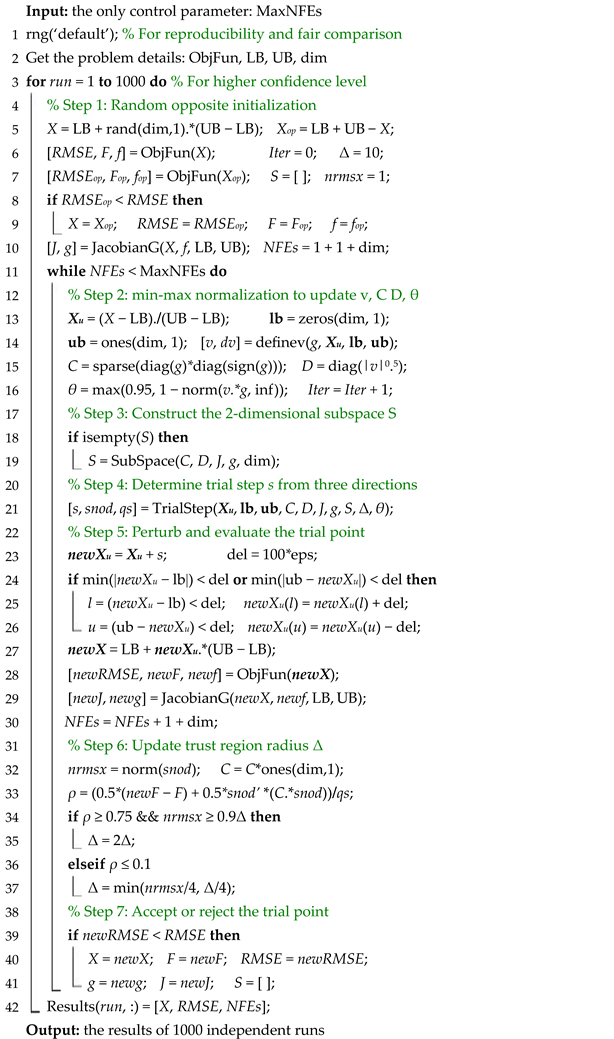
To overcome the above shortcomings of the standard TRR search, this paper adds two concepts, opposition-based learning (OBL) [34] and min-max normalization [35], to formulate the proposed ONTRR algorithm. The concept of OBL is used to produce a better initial point for the TRR search, while min-max normalization is applied to eliminate the negative effects arising from different magnitudes of model parameter values and thus to drive the derivative-dependent TRR search in an efficient manner. These two amendments are interspersed in the main routine illustrated in Algorithm 1. As can be seen from Algorithm 1, the proposed ONTRR algorithm begins by inputting the only control parameter MaxNFEs and specifying the default random seeds for solving the parameter extraction problem over 1000 independent runs. This is followed by:

Step 1: Random opposite initialization: generate a random point and its opposite point to obtain the initial point of the subsequent iteration loop.

Step 2: min-max normalization processing: generate the unitary surrogates of model parameter values to update the distances to the normalized boundary.

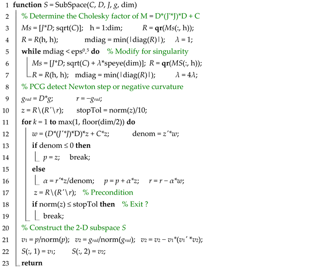
Step 3: Construct the 2-D subspace by Cholesky factorization and the preconditioned conjugate gradient method.

Step 4: Determine the trial step s from three directions via 2-D eigenvalue decomposition and one-dimensional reflective path search.

Step 5: Perturb the trial point to ensure it is not on the boundary and thus strictly feasible, and then return it to the original space for evaluating the error function.

Step 6: Update the trust region radius with Equations (13) and (19).

Step 7: Decide to accept or reject the trial point and update the Jacobian matrix, gradient and 2-D subspace for the next iteration.

The iteration loop incorporating Steps 2–7 is repeated until the terminate criterion MaxNFEs is reached. In the following subsections, the details of Steps 1–4 are explained.

Algorithm 1: Opposite normalized trust-region reflective

4.2. Step 1: Random Opposite Initialization

Unlike the standard TRR requiring the input of a good initial point, the proposed ONTRR adopts the concept of OBL to produce the opposite point X_op of a random point X within [LB, UB]. Then the better of these two points, that with a lower RMSE, is chosen as the initial point of the proposed ONTRR algorithm. It is evident from Figure 2 that, if the random point X is far away from the unknown optimum, its opposite point X_op should be closer to the unknown optimum. Hence, it is reasonable that initializing both X and X_op simultaneously will give a higher chance of finding the unknown optimum and reduce the probability of being trapped in local minima. This step is programmed in lines 5–10 of Algorithm 1, where rand(dim,1) is a dim-by-1 vector containing dim, a uniformly distributed random real number between 0 and 1, Δ = 10 is the initial trust region radius and nrmsx = 1 is the initial search step size, while the initial 2-D subspace S is set to be null. After invoking Algorithm 2 to calculate the Jacobian matrix J and gradient g at the initial point X, the number of the evaluating error function f reaches to NFEs = 2 + dim while the number of iterations is set to be Iter = 0, where eps is the floating-point relative accuracy and eye is the identity matrix.

Algorithm 2: Compute Jacobian matrix and gradient

Figure 2. The random point X and its opposite point X_op in one-dimensional space.

4.3. Step 2: Min-Max Normalization Processing to Update v, C, D and θ

For each iteration loop, firstly, the min-max normalization is employed to convert different data features into the same scales, as in lines 11–16 of Algorithm 1. Since the model parameter values in initial point X have different orders of magnitude, they are normalized to the unitary surrogate X_u with Equation (31). It is evident from Equation (31) that the boundaries LB and UB can be mapped with lb = zeros(dim,1) and ub = ones(dim, 1), respectively. Then X, LB and UB are replaced with their unitary surrogates X_u, lb and ub to update the distances to the normalized boundary using Equation (20) or the definev function of MATLAB.

$$X_u=\frac{X-\mathrm{LB}}{\mathrm{UB}-\mathrm{LB}}\in [0,1]$$

(31)

The role of min-max normalization processing is twofold. (1) To unify scale and dimensionless numbers to convert the model parameter values at different magnitudes into the same value range. (2) To improve the convergence rate of TRR search: since the model parameter values in X have different orders of magnitude, the gradients of I₀ or I_0i are significantly larger or smaller than those of other parameters. Consequently, the contour of the objective function is a flat ellipsoid rather than the ideal spherical shape, which will cause the gradient at most positions to deviate from the optimal search direction and thus make the derivative-dependent TRR search take more iterations to converge. Conversely, since the elements of unitary surrogate X_u are at the same scale and comparable, the gradients of all model parameters will be of the same order of magnitude. As a result, the gradient direction at most positions is similar to the optimal search direction, and the convergence rate of derivative-dependent ONTRR search will be greatly improved.

4.4. Step 3: Construct the Two-Dimensional Subspace S

In Algorithm 3, the subspace computing function starts with the Cholesky factorization of $\widehat{M}$ in Equation (22). If $\widehat{M}$ is positive definite, the Cholesky factor R will be immediately obtained by QR decomposition. If the factorization fails, which means $\widehat{M}$ is not positive definite, a direction of negative curvature is usually available. In lines 4–7 of Algorithm 3, the modification for singular $\widehat{M}$ is repeated until the smallest diagonal eigenvalue is larger than eps⁰.⁵, where λ is set to be 1 and speye returns a sparse identity matrix. With the aid of preconditioner R^TR and residual stopping tolerance stopTol, a PCG linear solver is carried out in lines 9–19 of Algorithm 3 to determine the inexact Newton direction or negative curvature direction by solving the local Newton system Equation (29) with no more than k_max = dim/2 CG iterations. For constructing the 2-D subspace S via Gram–Schmidt orthogonality, the last two lines of Algorithm 3 are slightly different from the trdog function of MATLAB, where the second direction v₂ of S is not always used unless its norm is larger than eps⁰.⁵.

Algorithm 3: Construct the two-dimensional subspace S

4.5. Step 4: Determine the Trial Step s from Three Directions

After creating the subspace S, the next thing is to determine the 2-D trust-region solution st. As with the standard TRR search, the proposed ONTRR algorithm employs the 2-D eigenvalue decomposition method to solve the secular Equation (27) and locate a feasible descent direction s, as is programmed in lines 3–4 of Algorithm 4. To ensure X_u + s is strictly feasible, the unconstrained trial step s, its affine scaling transformation ss and st are truncated by Equation (11) prior to calculating the quadratic approximation qs1, as is programmed in lines 6–7 of Algorithm 4. The truncate function in Algorithm 5 uses the normalized unitary surrogates X_u, lb and ub to calculate the min-max breakpoint distance mdis with Equation (16). Otherwise, it will cause great deviation from the optimal search direction. Moreover, since the step-back is controlled by θ, the truncated point along s is just close to but not at the breakpoint, as illustrated by the green and red points in Figure 3, respectively. Hence, prior to evaluating along the reflected direction s^R, we need to calculate the breakpoint with mdis and the untruncated st₀, ss₀ and s₀, as in lines 5, 9–12 of Algorithm 4, where δ = 0.9 is used to restrict the reflective step from being relatively too large [33]. As is evident from Figure 3, s and s^R are the same except for the component corresponding to the crossed constraint, where $s_i^R$ = $-s_i$ if that is the ith component [36]. Therefore, a simple one-dimensional reflective path search (using the quad1d function affiliated in the trdog function of MATLAB) can be performed to locate the improved direction ns and then truncate it to compute the quadratic approximation qs3, as in lines 13–19 of Algorithm 4. As for evaluating along the gradient direction, except for the extended gradient defined in line 21 of Algorithm 4 to protect against the possible degeneracy of $\widehat{g}$ = 0, the rest is similar to that of previous processes. Finally, the trial step is chosen from the best of three directions s, ns + s₀₁ and sg according to qs1, qs2 and qs3, respectively, as in lines 27–32 of Algorithm 4.

Algorithm 4: Determine the trial step s from three directions

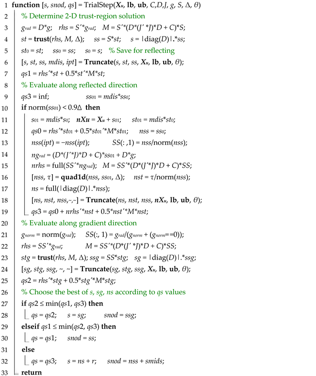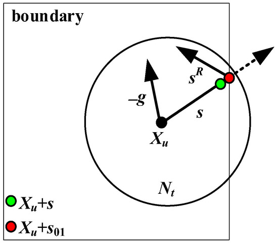
Figure 3. Reflecting and truncating the step s.

Algorithm 5: Truncate the trial step

4.6. Features and Control Parameter of ONTRR Algorithm

As can be seen from previous subsections, the random opposite initialization and the min-max normalization processing endow the proposed ONTRR with faster convergence speed and higher computation efficiency and make it robust enough to solve the problem of solar cell parameter extraction. Compared to the standard TRR search and ARC-TRR [29] algorithm, the proposed ONTRR algorithm exhibits two superiorities:

(1)

A good starting point is NOT necessary. With the help of Step 1, the user can randomly initialize the starting point without the aid of analytic methods or numerical methods, for example, the ABC algorithm given in reference [29].

(2)

Only one control parameter needs to be preset, i.e., the termination criterion MaxNFEs. This is a huge difference from the standard TRR search and ARC-TRR [29] algorithm, which have four and seven control parameters that have to be selected, respectively.

5. Experimental Results and Discussion

5.1. Experiment Settings

To verify the effectiveness of the proposed ONTRR algorithm, it was applied to solve the parameter extraction problem of benchmarked I–V datasets with the IEF- and LWF-based objective functions. The benchmarked I–V datasets are obtained from the output of an R.T.C. France cell at 33 °C, PWP201 module at 45 °C [37], STM6-40/36 module at 51 °C and STP6-120/36 module at 55 °C [38], which have been extensively adopted in the literature to test the performance of various algorithms. The parameter search ranges are maintained the same as in the previous literature and are listed in Table 1. To validate the advantages of the proposed ONTRR, it was compared with other state-of-the-art algorithms. To achieve a higher confidence level of comparison results, the proposed ONTRR and the most competitive algorithm ABC-TRR [29] are run independently for 1000 runs with default random seeds instead of the 30, 50, or 100 runs observed in most studies in the literature, a degree of diversity sufficient to ensure the results are objective and reproducible. The termination criterion MaxNFEs is set to be 1000, 5000 and 10,000 for parameter extraction of SDM, DDM and TDM, respectively. All comparative experiments were executed in MATLAB 2021b on a personal laptop with an Intel Core i7-1065G7 processor @1.30 GHz and 16 GB RAM running the Windows 10 64-bit OS.

Table 1. Operating temperature and parameter search ranges of four solar cells/modules.

Cell/Module	R.T.C. France Cell [37]	PWP201 Module [37]	STM6-40/36 Module [38]	STP6-120/36 Module [38]
T (°C)	33	45	51	55
Ns × Np	1 × 1	36 × 1	36 × 1	36 × 1
n, ni, nm	[1, 2]	[1, 50]	[1, 60]	[1, 50]
Iph, Iphm (A)	[0, 1]	[0, 2]	[0, 2]	[0, 8]
I0, I0i, I0m (A)	[0, 1 × 10−6]	[0, 50 × 10−6]	[0, 50 × 10−6]	[0, 50 × 10−6]
Rs, Rsm (Ω)	[0, 0.5]	[0, 2]	[0, 0.36]	[0, 0.36]
Rsh, Rshm (Ω)	[0, 100]	[0, 2000]	[0, 1000]	[0, 1500]

5.2. Solution Quality and Computational Efficiency

5.2.1. Six Cases Utilizing the IEF-Based Objective Function

The optimal results extracted from the IEF-based objective function by the proposed ONTRR are summarized in Table 2. To ensure that the reader can reproduce the RMSE values, the parameter values in Table 2 are correct to 8 decimal places and compared to the results of some state-of-the-art algorithms, such as EJBO [5], GSK [6], GNDO [7], CLRao−1 [8], IGSK [9], IMPA [10], EOTLBO [11], ELBA [12], QRMSCS [13], MIGTO [14], CPMPSO [15], GOFANM [16], WLCSODGM [17], ISCE [18], DOLADE [19], Rcr-IJADE [20], DPDE [21], HDE [22], EJADE [23], ISMA [24], DE/WOA [25], QNMPO [26], LNMHGS [27], EHA-NMS [28] and ABC-TRR [29]. By crosschecking Table 2 and the results in [5,6,7,8,9,10,11,12,13,14,15,16,17,18,19,20,21,22,23,24,25,26,27,28,29], one can find that there is a less than 0.01 percent differences between them, even though they include different numbers of decimal places. This means that the proposed ONTRR possesses identical accuracy to the compared algorithms. However, considering the consumed number of function evaluations (NFEs), it is evident from Figure 4 that only ONTRR and ABC-TRR always take the least NFEs to achieve the optimal RMSE values among all compared algorithms. This suggests that these two algorithms need the least computational effort to reach the same accuracy, thereby having the highest computational efficiency for parameter extraction of the IEF-based SDM, DDM and TDM, followed by the ISCE [18], EHA-NMS [28] and Rcr-IJADE [20] algorithms.

Table 2. Optimal results extracted from the IEF-based objective function by ONTRR algorithm.

Cell/Module	R.T.C. France Cell			PWP201 Module	STM6-40/36 Module	STP6-120/36 Module
Model	SDM	DDM	TDM	SDM	SDM	SDM
n, n1, nm	1.48118359	1.45101671	2.00000000	48.64283466	1.52030292	1.26010347
n2		2.00000000	2.00000000
n3			1.45101679
Iph, Iphm (A)	0.76077553	0.76078108	0.76078108	1.03051430	1.66390478	7.47252992
I0, I01, I0m (μA)	0.32302080	0.22597412	0.57680977	3.48226273	1.73865682	2.33499484
I02 (A)		0.74934873	0.17253702
I03 (A)			0.22597433
Rs, Rsm (mΩ)	36.37709278	36.74043067	36.74042998	1201.27101346	4.27377143	4.59463464
Rsh, Rshm (Ω)	53.71852462	55.48544266	55.48543523	981.98216392	15.92829404	22.21989981
RMSE	9.860219 × 10−4	9.824849 × 10−4	9.824849 × 10−4	2.425075 × 10−3	1.729814 × 10−3	1.660060 × 10−2
MaxNFEs	1000	5000	10,000	1000	1000	1000

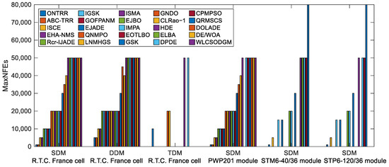
Figure 4. The consumed MaxNFEs of various algorithms with the IEF-based objective function.

5.2.2. Six Cases Utilizing the LWF-Based Objective Function

Table 3 lists the optimal results extracted from the LWF-based objective function by the ONTRR algorithm. It is evident from Table 3 and [4,39] that for all six cases, there is a less than 1% difference between the parameters of the ONTRR, RaAOA and MNMS algorithms, while the RMSE values of the ONTRR algorithm are less than or equal to those of the RaAOA and MNMS algorithms. As far as the consumed NFEs are concerned, for SDM, DDM and TDM, the MaxNFEs of the ONTRR algorithm are 1000, 5000 and 10,000, which are much less than the 5000, 30,000 and 30,000 of the MNMS and RaAOA algorithms. These results confirm that the proposed ONTRR algorithm consistently achieves the highest computational efficiency in extracting the most accurate parameter values of LWF-based SDM, DDM and TDM.

Table 3. Optimal results extracted from the LWF-based objective function by ONTRR algorithm.

Cell/Module	R.T.C. France Cell			PWP201 Module	STM6-40/36 Module	STP6-120/36 Module
Model	SDM	DDM	TDM	SDM	SDM	SDM
n, n1, nm	1.47726779	1.31093877	1.01967259	47.59822350	1.52046669	1.24445622
n2		1.84426858	1.04486626
n3			1.87876348
Iph, Iphm (A)	0.76078797	0.76119223	0.76171411	1.03143382	1.66390345	7.47528407
I0, I01, I0m (μA)	0.31068461	0.01984383	3.08359786 × 10−6	2.63807677	1.74124582	1.93088845
I02 (A)		1.00000000	7.72676991 × 10−5
I03 (A)			1.00000000
Rs, Rsm (mΩ)	36.54694512	65.31374450	111.12052185	1235.63416949	4.26778393	4.69217169
Rsh, Rshm (Ω)	52.88979013	56.52733441	63.71629154	821.64129780	15.93149782	15.83882138
RMSE	7.730063 × 10−4	6.745134 × 10−4	5.837513 × 10−4	2.052961 × 10−3	1.721922 × 10−3	1.425106 × 10−2
MaxNFEs	1000	5000	10,000	1000	1000	1000

5.2.3. Accuracy Difference and Model Degeneration

Two points can be drawn from Table 2 and Table 3. Firstly, the parameters extracted from the LWF-based objective function are more accurate than those extracted from the IEF-based objective function. The basic reason is that the implicit nature of Equation (6) increases the difficulty of parameter extraction, while Equation (7) is an approximate explicit expression. Secondly, the IEF-based objective function is prone to model degeneration. One can see from Table 2 that the TDM parameters satisfy n₁ = n₂, which can also be found for the LNMHGS [27] algorithm. In addition, the TDM parameters extracted by the HDE [22] algorithm meet n₁ = n₃, while the DPDE [21] algorithm yields I₀₃ ≈ 0. These make the IEF-based TDM degenerate into that of DDM, as evidenced by the identical RMSE values in Table 2. It is clear from Figure 5 that, although both the IEF- and LWF-based simulated current data are in good agreement with the measured current data, there are still visible differences between them. For the IEF-based cases in Figure 5b,c, the simulated current data and the sum of individual absolute errors (IAE_IEF) of TDM are identical to those of DDM. These results support the aforementioned statements about accuracy difference and model degeneration.

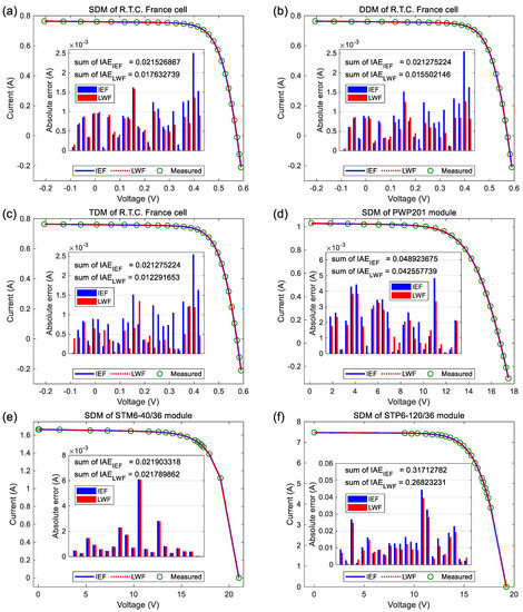
Figure 5. Simulated currents obtained by the IEF- and LWF-based parameters of ONTRR algorithm. (a) SDM of R.T.C. France cell. (b) DDM of R.T.C. France cell, (c) TDM of R.T.C. France cell, (d) SDM of PWP201 module, (e) SDM of STM6-40/36 module and (f) SDM of STP6-120/36 module.

5.3. Convergence Speed

5.3.1. Convergence for the IEF-Based Objective Function

The average convergence curves of 1000 independent runs of the ONTRR and ABC-TRR algorithms are plotted in Figure 6 for comparison with the reported results of the ISCE and EHA-NMS algorithms. For the five cases excluding TDM, the average convergence curves of ONTRR lie to the lower left of those of ABC-TRR, followed by the ISCE and EHA-NMS curves. The final average RMSE values (i.e., average accuracy) of ONTRR are less than or equal to those of the other algorithms, as the DataTips in Figure 6a,b,d,f show. Hence, the convergence speed can be sorted as ONTRR > ABC-TRR > ISCE > EHA-NMS. For the TDM case, the zoomed-in view in Figure 6c indicates that the average convergence curve of ABC-TRR is lower than that of ONTRR in the later period. This proves that ONTRR converges slightly slower than ABC-TRR for solving the IEF-based parameter extraction problem of TDM.

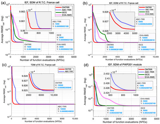
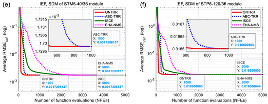
Figure 6. Average convergence graphs of 1000 independent runs of different algorithms for parameter extraction of the IEF-based single, double and triple diode models. (a) SDM of R.T.C. France cell. (b) DDM of R.T.C. France cell, (c) TDM of R.T.C. France cell, (d) SDM of PWP201 module, (e) SDM of STM6-40/36 module and (f) SDM of STP6-120/36 module.

5.3.2. Convergence for the LWF-Based Objective Function

Figure 7 illustrates the average convergence curves of 1000 independent runs of the ONTRR and ABC-TRR algorithms during the parameter extraction process of the LWF-based objective function. For all the six cases in Figure 7a–f, the average convergence curves of ONTRR consistently lie to the lower left of those of ABC-TRR, and the final average RMSE values of ONTRR are less than or equal to those of ABC-TRR. This confirms that the proposed ONTRR algorithm converges faster than ABC-TRR for solving the LWF-based parameter extraction problem of SDM, DDM and TDM.

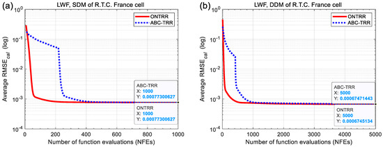
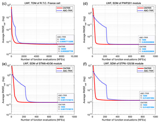
Figure 7. Average convergence graphs of 1000 independent runs of two algorithms for parameter extraction of the LWF-based single, double and triple diode models. (a) SDM of R.T.C. France cell. (b) DDM of R.T.C. France cell, (c) TDM of R.T.C. France cell, (d) SDM of PWP201 module, (e) SDM of STM6-40/36 module and (f) SDM of STP6-120/36 module.

5.3.3. Convergence at the Threshold Value of RMSE

The statistical results of 1000 independent runs of the ONTRR algorithm are summarized in Table 4 and Table 5, where the indicator NFEs@thV is employed to quantify the convergence performance. NFEs@thV records the consumed NFEs when RMSE reaches a threshold value (thV). For all twelve cases, it is evident from Table 4 and Table 5 that the mean NFEs@thV of ONTRR are markedly smaller than those of ABC-TRR and much less than those of ISCE, EHA-NMS and R_cr-IJADE. It can be computed from Table 4 and Table 5 that the ratios of mean NFEs@thV between ABC-TRR and ONTRR algorithms are 1.98, 2.45, 3.02, 3.41, 1.97, 2.54 and 3.25, 2.45, 2.48, 5.86, 2.84, 4.09, respectively. Hence, it can be seen that the average convergence improvement is 3.03 times in comparison with the best-performing algorithms reporting in the literature.

Table 4. Statistical results of 1000 independent runs of five algorithms for parameter extraction of the IEF-based single, double and triple diode models.

Algorithms	MaxNFEs	Final RMSE				NFEs@thV
		Min	Mean	Max	Std (Rank)	Min	Mean	Max	Std (Rank)
R.T.C. France cell, SDM, thV = 0.001
ONTRR	1000	9.860219 × 10−4	9.860219 × 10−4	9.860219 × 10−4	6.81 × 10−17 (4)	29	200	670	89 (1)
ABC-TRR [29]	1000	9.860219 × 10−4	9.860219 × 10−4	9.860219 × 10−4	6.38 × 10−17 (2)	231	395	806	94 (2)
ISCE [18]	5000	9.860219 × 10−4	9.860219 × 10−4	9.860219 × 10−4	3.98 × 10−17 (1)	505	2072	3830	644 (4)
EHA-NMS [28]	5000	9.860219 × 10−4	9.860219 × 10−4	9.860219 × 10−4	6.64 × 10−17 (3)	705	1755	3527	475 (3)
Rcr-IJADE [20]	10,000	9.860219 × 10−4	9.860219 × 10−4	9.860219 × 10−4	3.10 × 10−14 (5)	2586	4735	6534	948 (5)
R.T.C. France cell, DDM, thV = 0.001
ONTRR	5000	9.824849 × 10−4	9.826189 × 10−4	9.860248 × 10−4	6.72 × 10−7 (3)	33	314	2316	174 (2)
ABC-TRR [29]	5000	9.824849 × 10−4	9.826490 × 10−4	9.871624 × 10−4	7.47 × 10−7 (4)	433	770	1262	166 (1)
ISCE [18]	10,000	9.824849 × 10−4	9.827740 × 10−4	9.861092 × 10−4	4.61 × 10−7 (1)	911	2122	5379	757 (3)
EHA-NMS [28]	10,000	9.824849 × 10−4	9.826829 × 10−4	9.860219 × 10−4	5.19 × 10−7 (2)	1477	2908	8012	848 (4)
Rcr-IJADE [20]	20,000	9.824849 × 10−4	9.833549 × 10−4	9.860234 × 10−4	1.20 × 10−6 (5)	3874	6523	15742	1551 (5)
R.T.C. France cell, TDM, thV = 0.001
ONTRR	10,000	9.824849 × 10−4	9.825085 × 10−4	9.894177 × 10−4	3.18 × 10−7 (2)	51	364	2111	178 (1)
ABC-TRR [29]	10,000	9.824849 × 10−4	9.824902 × 10−4	9.878124 × 10−4	1.68 × 10−7 (1)	637	1099	2674	225 (2)
PWP201 module, SDM, thV = 0.01
ONTRR	1000	2.425075 × 10−3	2.425075 × 10−3	2.425075 × 10−3	6.66 × 10−17 (4)	16	66	153	24 (2)
ABC-TRR [29]	1000	2.425075 × 10−3	2.425075 × 10−3	2.425075 × 10−3	1.73 × 10−16 (5)	108	227	311	9 (1)
ISCE [18]	5000	2.425075 × 10−3	2.425075 × 10−3	2.425075 × 10−3	2.47 × 10−17 (1)	107	303	566	41 (3)
EHA-NMS [28]	5000	2.425075 × 10−3	2.425075 × 10−3	2.425075 × 10−3	5.53 × 10−17 (3)	468	1113	2237	344 (5)
Rcr-IJADE [20]	10,000	2.425075 × 10−3	2.425075 × 10−3	2.425075 × 10−3	2.51 × 10−17 (2)	580	1200	1654	204 (4)
STM6-40/36 module, SDM, thV = 0.002
ONTRR	1000	1.729814 × 10−3	1.729814 × 10−3	1.729814 × 10−3	3.26 × 10−17 (3)	34	152	456	53 (1)
ABC-TRR [29]	1000	1.729814 × 10−3	1.729814 × 10−3	1.729814 × 10−3	9.43 × 10−17 (4)	223	299	724	63 (2)
ISCE [18]	5000	1.729814 × 10−3	1.729814 × 10−3	1.729814 × 10−3	2.30 × 10−17 (1)	397	1122	2575	449 (4)
EHA-NMS [28]	5000	1.729814 × 10−3	1.729814 × 10−3	1.729814 × 10−3	2.43 × 10−17 (2)	888	1645	2705	311 (3)
Rcr-IJADE [20]	10,000	1.729814 × 10−3	1.729814 × 10−3	1.729814 × 10−3	1.18 × 10−14 (5)	1732	2972	4780	606 (5)
STP6-120/36 module, SDM, thV = 0.02
ONTRR	1000	1.660060 × 10−2	1.660060 × 10−2	1.660060 × 10−2	3.32 × 10−15 (1)	25	120	582	57 (1)
ABC-TRR [29]	1000	1.660060 × 10−2	1.660060 × 10−2	1.660060 × 10−2	1.22 × 10−14 (2)	221	305	770	79 (2)
ISCE [18]	5000	1.660060 × 10−2	1.660060 × 10−2	1.660060 × 10−2	8.74 × 10−14 (4)	320	788	1594	246 (4)
EHA-NMS [28]	5000	1.660060 × 10−2	1.660064 × 10−2	1.664184 × 10−2	1.30 × 10−6 (5)	787	1216	2050	231 (3)
Rcr-IJADE [20]	10,000	1.660060 × 10−2	1.660060 × 10−2	1.660060 × 10−2	1.29 × 10−14 (3)	1471	2562	3644	490 (5)

Table 5. Statistical results of 1000 independent runs of two algorithms for parameter extraction of the LWF-based single, double and triple diode models.

Algorithms	MaxNFEs	Final RMSE				NFEs@thV
		Min	Mean	Max	Std (Rank)	Min	Mean	Max	Std (Rank)
R.T.C. France cell, SDM, thV = 0.001
ONTRR	1000	7.730063 × 10−4	7.730063 × 10−4	7.730063 × 10−4	7.06 × 10−17 (1)	22	92	716	65 (1)
ABC-TRR [29]	1000	7.730063 × 10−4	7.730063 × 10−4	7.730063 × 10−4	1.99 × 10−16 (2)	224	299	789	70 (2)
R.T.C. France cell, DDM, thV = 0.001
ONTRR	5000	6.745134 × 10−4	6.745134 × 10−4	6.745134 × 10−4	1.25 × 10−16 (1)	25	277	629	129 (1)
ABC−TRR [29]	5000	6.745134 × 10−4	6.747121 × 10−4	7.661344 × 10−4	4.12 × 10−6 (2)	427	681	1199	152 (2)
R.T.C. France cell, TDM, thV = 0.001
ONTRR	10,000	5.837513 × 10−4	6.267755 × 10−4	7.602632 × 10−4	6.09 × 10−5 (1)	63	431	1150	180 (1)
ABC-TRR [29]	10,000	5.838190 × 10−4	6.769198 × 10−4	7.674062 × 10−4	6.75 × 10−5 (2)	631	1066	2547	265 (2)
PWP201 module, SDM, thV = 0.01
ONTRR	1000	2.052961 × 10−3	2.052961 × 10−3	2.052961 × 10−3	1.57 × 10−16 (1)	15	38	77	7 (1)
ABC-TRR [29]	1000	2.052961 × 10−3	2.052961 × 10−3	2.052961 × 10−3	2.19 × 10−15 (2)	87	225	266	8 (2)
STM6-40/36 module, SDM, thV = 0.002
ONTRR	1000	1.721922 × 10−3	1.721922 × 10−3	1.721922 × 10−3	3.73 × 10−17 (1)	33	102	467	39 (1)
ABC-TRR [29]	1000	1.721922 × 10−3	1.721922 × 10−3	1.721922 × 10−3	1.89 × 10−16 (2)	222	291	697	55 (2)
STP6-120/36 module, SDM, thV = 0.02
ONTRR	1000	1.425106 × 10−2	1.425106 × 10−2	1.425106 × 10−2	8.30 × 10−15 (1)	18	63	461	35 (1)
ABC-TRR [29]	1000	1.425106 × 10−2	1.425106 × 10−2	1.425106 × 10−2	5.49 × 10−14 (2)	222	258	661	43 (2)

5.4. Statistic Stability

In Table 4 and Table 5, the rank of standard deviations (Std) is used to quantify the stability of the final RMSE values and NFEs@thV of five compared algorithms. It can be computed from Table 4 that for the five IEF-based cases excluding TDM, the sum of ranks (SR) achieved by the ONTRR, ABC-TRR, ISCE, EHA-NMS and R_cr-IJADE algorithms are 22, 25, 26, 33 and 44, respectively. Considering the fact that, for the TDM case, the SR value of ONTRR is identical to that of ABC-TRR, the statistic stability of the five algorithms can be sorted as ONTRR > ABC-TRR > ISCE > EHA-NMS > R_cr-IJADE. For the six LWF-based cases, it is evident from Table 5 that all the Stds and ranks of ONTRR are smaller than those of ABC-TRR. Hence, the proposed ONTRR is statistically more stable than the ABC-TRR algorithm.

5.5. Overall Performance

For all twelve of the cases in Table 4 and Table 5, a Friedman test with a confidence of 0.05 is used to evaluate the overall performances of the five compared algorithms. The Friedman test ranks each indicator and then gives the average rank of each algorithm. It is clear from the left of Figure 8 that the average rank of ONTRR is better than that of ABC-TRR. For the five IEF-based cases excluding TDM, it is evident from the right of Figure 8 that ONTRR still ranks the best on average, followed by ABC-TRR, ISCE, EHA-NMS and R_cr-IJADE. These results confirm that the proposed ONTRR outperforms other algorithms in extracting the most accurate parameter values of IEF- and LWF-based solar cell models.

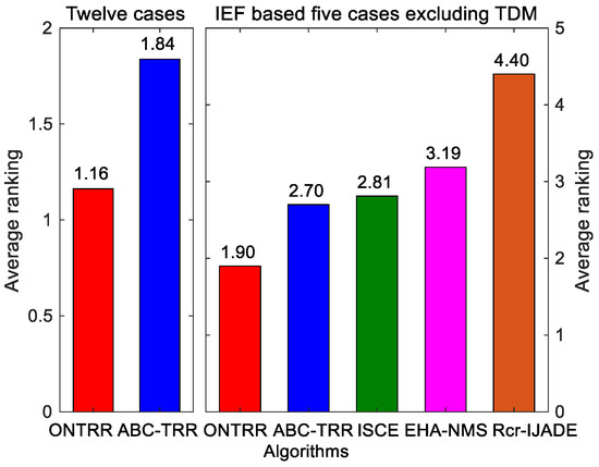
Figure 8. Friedman test results of the five compared algorithms.

6. Conclusions and Future Works

In this paper, a randomly initialized, derivative-dependent algorithm ONTRR is proposed to improve the parameter extraction of solar cell models. The proposed ONTRR embeds OBL and min-max normalization into the standard TRR search to overcome the deficiencies of the latter of being sensitive to the initial point and different scale model parameter values. As an improved version of the standard TRR search, the proposed ONTRR algorithm has only one control parameter and is envisaged to accurately, efficiently and reliably extract the unknown parameters of SDM, DDM and TDM.

The proposed ONTRR algorithm is comprehensively tested and compared with the best-performing algorithms in the literature (such as ABC-TRR, ISCE, EHA-NMS, etc.) using four benchmarked I–V datasets with the IEF- and LWF-based objective functions. To be objective and reproducible, the proposed ONTRR algorithm is run independently 1000 times with default random seeds to investigate its convergence speed, average accuracy and statistic stability. The comparison results of twelve test cases confirm the outperformance of ONTRR. (1) In terms of solution quality and computational efficiency, the proposed ONTRR consistently achieves the highest accuracy with the least computational effort among all the compared algorithms. (2) In terms of convergence speed and average accuracy of 1000 independent runs, the proposed ONTRR surpasses other algorithms in most cases. The average convergence improvement is 3.03 times in comparison to the best-performing algorithms reported in the literature. (3) In terms of statistics stability of 1000 independent runs, the sum of ranks of standard deviation achieved by the proposed ONTRR is much less than that of the other algorithms. (4) In terms of overall performance, the average rank of ONTRR is better than those of the other algorithms. Given these superiorities, the proposed ONTRR is expected to be the most promising option for solar cell parameter extraction.

In this paper, the proposed ONTRR algorithm is only used to extract the model parameters from the measured I–V data under the given operating condition. For future work, it will be extended to explore the dependence of extracted parameters on the input irradiances and temperatures for fault detection, maximum power point tracking and energy yield predictions of PV systems and solving other complex problems.

References

- Femia, N.; Spagnuolo, G.; Vitelli, M. Power Electronics and Control Techniques for Maximum Energy Harvesting in Photovoltaic Systems; Bogdan, M., Wilamowski, Irwin, J.D., Eds.; CRC Press, Taylor & Francis Group: Boca Raton, FL, USA, 2013. [Google Scholar]
- Li, S.; Gong, W.; Gu, Q. A Comprehensive Survey on Meta-Heuristic Algorithms for Parameter Extraction of Photovoltaic Models. Renew. Sustain. Energy Rev. 2021, 141, 110828. [Google Scholar] [CrossRef]
- Ridha, H.M.; Hizam, H.; Mirjalili, S.; Othman, M.L.; Ya’acob, M.E.; Ahmadipour, M. Parameter Extraction of Single, Double, and Three Diodes Photovoltaic Model Based on Guaranteed Convergence Arithmetic Optimization Algorithm and Modified Third Order Newton Raphson Methods. Renew. Sustain. Energy Rev. 2022, 162, 112436. [Google Scholar] [CrossRef]
- Mohammed Ridha, H.; Hizam, H.; Mirjalili, S.; Lutfi Othman, M.; Effendy Ya’acob, M.; Ahmadipour, M. Novel Parameter Extraction for Single, Double, and Three Diodes Photovoltaic Models Based on Robust Adaptive Arithmetic Optimization Algorithm and Adaptive Damping Method of Berndt-Hall-Hall-Hausman. Sol. Energy 2022, 243, 35–61. [Google Scholar] [CrossRef]
- Ahmadianfar, I.; Gong, W.; Heidari, A.A.; Golilarz, N.A.; Samadi-Koucheksaraee, A.; Chen, H. Gradient-Based Optimization with Ranking Mechanisms for Parameter Identification of Photovoltaic Systems. Energy Rep. 2021, 7, 3979–3997. [Google Scholar] [CrossRef]
- Xiong, G.; Li, L.; Mohamed, A.W.; Yuan, X.; Zhang, J. A New Method for Parameter Extraction of Solar Photovoltaic Models Using Gaining–Sharing Knowledge Based Algorithm. Energy Rep. 2021, 7, 3286–3301. [Google Scholar] [CrossRef]
- Zhang, Y.; Jin, Z.; Mirjalili, S. Generalized Normal Distribution Optimization and Its Applications in Parameter Extraction of Photovoltaic Models. Energy Convers. Manag. 2020, 224, 113301. [Google Scholar] [CrossRef]
- Farah, A.; Belazi, A.; Benabdallah, F.; Almalaq, A.; Chtourou, M.; Abido, M.A. Parameter Extraction of Photovoltaic Models Using a Comprehensive Learning Rao-1 Algorithm. Energy Convers. Manag. 2022, 252, 115057. [Google Scholar] [CrossRef]
- Sallam, K.M.; Hossain, M.A.; Chakrabortty, R.K.; Ryan, M.J. An Improved Gaining-Sharing Knowledge Algorithm for Parameter Extraction of Photovoltaic Models. Energy Convers. Manag. 2021, 237, 114030. [Google Scholar] [CrossRef]
- Abdel-Basset, M.; El-Shahat, D.; Chakrabortty, R.K.; Ryan, M. Parameter Estimation of Photovoltaic Models Using an Improved Marine Predators Algorithm. Energy Convers. Manag. 2021, 227, 113491. [Google Scholar] [CrossRef]
- Xiong, G.; Zhang, J.; Shi, D.; Zhu, L.; Yuan, X. Parameter Extraction of Solar Photovoltaic Models with an Either-or Teaching Learning Based Algorithm. Energy Convers. Manag. 2020, 224, 113395. [Google Scholar] [CrossRef]
- Deotti, L.M.P.; Pereira, J.L.R.; da Silva, I.C., Jr. Parameter Extraction of Photovoltaic Models Using an Enhanced Lévy Flight Bat Algorithm. Energy Convers. Manag. 2020, 221, 113114. [Google Scholar] [CrossRef]
- Luo, W.; Yu, X. Quasi-Reflection Based Multi-Strategy Cuckoo Search for Parameter Estimation of Photovoltaic Solar Modules. Sol. Energy 2022, 243, 264–278. [Google Scholar] [CrossRef]
- Abdel-Basset, M.; El-Shahat, D.; Sallam, K.M.; Munasinghe, K. Parameter Extraction of Photovoltaic Models Using a Memory-Based Improved Gorilla Troops Optimizer. Energy Convers. Manag. 2022, 252, 115134. [Google Scholar] [CrossRef]
- Liang, J.; Ge, S.; Qu, B.; Yu, K.; Liu, F.; Yang, H.; Wei, P.; Li, Z. Classified Perturbation Mutation Based Particle Swarm Optimization Algorithm for Parameters Extraction of Photovoltaic Models. Energy Convers. Manag. 2020, 203, 112138. [Google Scholar] [CrossRef]
- Xu, S.; Wang, Y. Parameter Estimation of Photovoltaic Modules Using a Hybrid Flower Pollination Algorithm. Energy Convers. Manag. 2017, 144, 53–68. [Google Scholar] [CrossRef]
- Xiong, G.; Zhang, J.; Shi, D.; Zhu, L.; Yuan, X.; Tan, Z. Winner-Leading Competitive Swarm Optimizer with Dynamic Gaussian Mutation for Parameter Extraction of Solar Photovoltaic Models. Energy Convers. Manag. 2020, 206, 112450. [Google Scholar] [CrossRef]
- Gao, X.; Cui, Y.; Hu, J.; Xu, G.; Wang, Z.; Qu, J.; Wang, H. Parameter Extraction of Solar Cell Models Using Improved Shuffled Complex Evolution Algorithm. Energy Convers. Manag. 2018, 157, 460–479. [Google Scholar] [CrossRef]
- Zhou, J.; Zhang, Y.; Zhang, Y.; Shang, W.-L.; Yang, Z.; Feng, W. Parameters Identification of Photovoltaic Models Using a Differential Evolution Algorithm Based on Elite and Obsolete Dynamic Learning. Appl. Energy 2022, 314, 118877. [Google Scholar] [CrossRef]
- Gong, W.; Cai, Z. Parameter Extraction of Solar Cell Models Using Repaired Adaptive Differential Evolution. Sol. Energy 2013, 94, 209–220. [Google Scholar] [CrossRef]
- Gao, S.; Wang, K.; Tao, S.; Jin, T.; Dai, H.; Cheng, J. A State-of-the-Art Differential Evolution Algorithm for Parameter Estimation of Solar Photovoltaic Models. Energy Convers. Manag. 2021, 230, 113784. [Google Scholar] [CrossRef]
- Wang, D.; Sun, X.; Kang, H.; Shen, Y.; Chen, Q. Heterogeneous Differential Evolution Algorithm for Parameter Estimation of Solar Photovoltaic Models. Energy Rep. 2022, 8, 4724–4746. [Google Scholar] [CrossRef]
- Li, S.; Gu, Q.; Gong, W.; Ning, B. An Enhanced Adaptive Differential Evolution Algorithm for Parameter Extraction of Photovoltaic Models. Energy Convers. Manag. 2020, 205, 112443. [Google Scholar] [CrossRef]
- Weng, X.; Heidari, A.A.; Liang, G.; Chen, H.; Ma, X. An Evolutionary Nelder–Mead Slime Mould Algorithm with Random Learning for Efficient Design of Photovoltaic Models. Energy Rep. 2021, 7, 8784–8804. [Google Scholar] [CrossRef]
- Xiong, G.; Zhang, J.; Yuan, X.; Shi, D.; He, Y.; Yao, G. Parameter Extraction of Solar Photovoltaic Models by Means of a Hybrid Differential Evolution with Whale Optimization Algorithm. Sol. Energy 2018, 176, 742–761. [Google Scholar] [CrossRef]
- Xu, B.; Heidari, A.A.; Kuang, F.; Zhang, S.; Chen, H.; Cai, Z. Performance Optimization of Photovoltaic Systems: Reassessment of Political Optimization with a Quantum Nelder-Mead Functionality. Sol. Energy 2022, 234, 39–63. [Google Scholar] [CrossRef]
- Yu, S.; Heidari, A.A.; He, C.; Cai, Z.; Althobaiti, M.M.; Mansour, R.F.; Liang, G.; Chen, H. Parameter Estimation of Static Solar Photovoltaic Models Using Laplacian Nelder-Mead Hunger Games Search. Sol. Energy 2022, 242, 79–104. [Google Scholar] [CrossRef]
- Chen, Z.; Wu, L.; Lin, P.; Wu, Y.; Cheng, S. Parameters Identification of Photovoltaic Models Using Hybrid Adaptive Nelder-Mead Simplex Algorithm Based on Eagle Strategy. Appl. Energy 2016, 182, 47–57. [Google Scholar] [CrossRef]
- Wu, L.; Chen, Z.; Long, C.; Cheng, S.; Lin, P.; Chen, Y.; Chen, H. Parameter Extraction of Photovoltaic Models from Measured I-V Characteristics Curves Using a Hybrid Trust-Region Reflective Algorithm. Appl. Energy 2018, 232, 36–53. [Google Scholar] [CrossRef]
- Chen, Z.; Wu, L.; Cheng, S.; Lin, P.; Wu, Y.; Lin, W. Intelligent Fault Diagnosis of Photovoltaic Arrays Based on Optimized Kernel Extreme Learning Machine and I-V Characteristics. Appl. Energy 2017, 204, 912–931. [Google Scholar] [CrossRef]
- Coleman, T.F.; Li, Y. An Interior Trust Region Approach for Nonlinear Minimization Subject to Bounds. SIAM J. Optim. 1996, 6, 418–445. [Google Scholar] [CrossRef]
- Branch, M.A.N.N.; Coleman, T.F. A Subspace, Interior, and Conjugate Gradient Method for Large-Scale Bound-Constrained Minimization Problems. SIAM J. Sci. Comput. 1999, 21, 1–23. [Google Scholar] [CrossRef]
- Coleman, T.F.; Li, Y. A Reflective Newton Method for Minimizing a Quadratic Function Subject to Bounds on Some of the Variables. SIAM J. Optim. 1996, 6, 1040–1058. [Google Scholar] [CrossRef]
- Mahdavi, S.; Rahnamayan, S.; Deb, K. Opposition Based Learning: A Literature Review. Swarm Evol. Comput. 2018, 39, 1–23. [Google Scholar] [CrossRef]
- Vafaei, N.; Ribeiro, R.A.; Camarinha-Matos, L.M. Assessing Normalization Techniques for Simple Additive Weighting Method. Procedia Comput. Sci. 2022, 199, 1229–1236. [Google Scholar] [CrossRef]
- Branch, M.A. Inexact Reflective Newton Methods for Large-Scale Optimization Subject to Bound Constraints; Cornell University: Ithaca, NY, USA, 1996. [Google Scholar]
- Easwarakhanthan, T.; Bottin, J.; Bouhouch, I.; Boutrit, C. Nonlinear Minimization Algorithm for Determining the Solar Cell Parameters with Microcomputers. Int. J. Sol. Energy 1986, 4, 1–12. [Google Scholar] [CrossRef]
- Tong, N.T.; Pora, W. A Parameter Extraction Technique Exploiting Intrinsic Properties of Solar Cells. Appl. Energy 2016, 176, 104–115. [Google Scholar] [CrossRef]
- Gao, X.; Cui, Y.; Hu, J.; Tahir, N.; Xu, G. Performance Comparison of Exponential, Lambert W Function and Special Trans Function Based Single Diode Solar Cell Models. Energy Convers. Manag. 2018, 171, 1822–1842. [Google Scholar] [CrossRef]
Disclaimer/Publisher’s Note: The statements, opinions and data contained in all publications are solely those of the individual author(s) and contributor(s) and not of MDPI and/or the editor(s). MDPI and/or the editor(s) disclaim responsibility for any injury to people or property resulting from any ideas, methods, instructions or products referred to in the content. |
© 2023 by the authors. Licensee MDPI, Basel, Switzerland. This article is an open access article distributed under the terms and conditions of the Creative Commons Attribution (CC BY) license (https://creativecommons.org/licenses/by/4.0/).