Abstract
This article describes an innovative method for the determination of heat flow (specific heat loss; linear heat flow density) from a one-metre length of a twin pipe directly-buried heat network. Such heat losses are currently described by applying analytical procedures based on the heat transfer theory. It is rather complicated to accurately express the heat loss using such procedures, due to the necessity to determine the individual values of thermal resistance. A simpler method to express heat loss is the balance method, as it requires measuring a temperature gradient Δt between the starting point of the heat network and the end point of the heat collection. A suitable measuring device must provide high-accuracy measurements of the temperature. In the case of very well-insulated distribution pipelines and short pipes, the temperature measurements must be accurate to the hundredths of a degree Celsius. It is impossible to install such devices as fixed equipment on every heat distribution network, due to such networks measuring many kilometres and the cost of the appropriate measuring technology. For the aforesaid reasons, the authors created a mathematical model for specific heat losses based on dimensional analysis. This method facilitates the identification of dimensionless criteria based on the relevant dimensional quantities. Functional correlations between the identified criteria may be identified on the basis of the results of physical or numerical experiments. In this study, a database of the results obtained from physical experiments conducted on two heat networks was used. The output of the similarity model was a function describing the heat flow from a one-meter pipe length that was applicable to various alternatives in relation to the geometrical, physical and boundary conditions. The standard deviation of a difference in the heat losses identified by applying the balance method and using the proposed criterial equation for a twin pipe directly-buried pre-insulated heat network was 0.515 W·m−1.
1. Introduction
Exact mathematical formulations for heat transfer in heat distribution systems are associated with certain shortcomings, which are related to the exact identification of the heat transfer coefficient for the external side of a directly-buried heat distribution pipeline.
A problem associated with identifying the heat loss in a directly-buried pipeline is that the cooling of the pipes is not a symmetrical process, especially in the case of a twin pipe arrangement. Differences in the heat removal in individual directions cause differences in the temperatures measured along the thickness of the insulation. The thermal conductivity coefficient, which has a significant effect on heat loss, also changes with a changing temperature.
The authors of this article, therefore, searched for a procedure that would facilitate the simplest possible description, but with sufficient accuracy, of the specific heat loss of a twin pipe directly-buried heat network. They conducted a precise experiment and created a similarity model based on dimensional analysis.
In order to find concrete quantities of a criterial equation, it is possible to use the results of an experiment or numerical simulations. The procedure for deriving a criterial equation by a dimensional analysis is described in detail in Section 3.
The authors of this article had extensive experience with even more complicated physical experiments [1,2]. In addition to physical experiments, tasks related to heat transfer and heat flow are also solved using a numerical simulation. For example, the authors of a publication [3] presented a similarity model for the description of the temperature of cooled fluid in cisterns relative to the transportation time, in which they used the results of an extensive numerical calculation. Numerical experiments are also used in specific fields of technology, with the use of various software products. For example, the finite element method (FEM), integrated with COMSOL Multiphysics software, was used in an investigation into the effects of adding nanoparticles of copper oxide during a heat transfer [4]. Furthermore, an investigation into a two-phase developing laminar mixing layer at supercritical pressures was carried out by applying the finite volume method (FVM) [5]. The FVM was also used in an investigation into the enhancement of a turbulent heat transfer in a mini-channel cooler [6] and in a study of loop heat pipes for heat transfers [7], as well as in various other applications of specific technical solutions [8,9,10,11,12,13].
2. Analysis of the Problem
To describe a process for which no exact physical equation exists, or if the application of a physical equation is assumed to be problematic, it is advisable to perform an experiment and to generalise its results while applying the laws of similarity. Similar processes that depend on several physical quantities are subject to certain correlations between the similarity constants, which cannot be arbitrarily changed [14,15,16,17,18,19]. Such a condition must also apply to a description of the specific heat loss for directly-buried heat distribution systems.
Following a detailed analysis, several physical quantities that affect the specific heat flow were selected for the twin pipe directly-buried heat network. The selected quantities relevant to the creation of a mathematical model using a dimensional analysis are listed in Table 1. In the process of creating a model law, the dimensions of physical quantities are always transformed to the seven SI units (kg; m; s; K; A; mol; cd). However, the quantities that are relevant to the creation of a model of specific heat loss are only four basic dimensions—kg, m, s and K.

Table 1.
Input quantities for the mathematical model.
The table does not contain the coefficient of heat transfer from the flowing fluid to the pipe wall α, internal diameter of the pipe d1, pipe wall thickness bp, and the thermal conductivity coefficient for the pipe wall λp. A detailed analysis, conducted for steel pipes through which hot water flowed at a rate of several metres per second, showed that the sum of the thermal resistance on the internal side of the pipe and the thermal resistance of the pipe wall was a value three orders lower than the value for the thermal resistance of the pipe insulation. Therefore, the quantities α, d1, bp and λp can be neglected in the creation of the model.
A similarity model for describing any phenomenon (a criterial equation) is created in the process of replacing selected dimensional quantities φ1 to φn with similarity criteria π1 to πl, and then by identifying functional correlations between the individual criteria either experimentally or by a numerical calculation. Such a criterial equation is then applicable to the entire group of similar phenomena.
A general procedure for applying dimensional analysis, in order to describe a process for which no exact analytical solution is known, is described in detail in papers [20,21,22]. The authors of this article applied dimensional analysis when describing the formation of nitrogen oxides during a dendromass combustion process. The resulting criterial equation was verified in a physical experiment, conducted on the combustion equipment by Werner with a power of 13 kW [23]. The results obtained from the model were in absolute agreement with the results obtained in situ using a HORYBA ENDA—680P analyser. The errors in the identification of nitrogen oxides by direct measurements and according to the created model ranged from −0.54 to +0.48%. The authors of this article also applied a dimensional analysis to modelling the prediction of nitrogen concentrations in the Laborec River in Slovakia [24]. A sensitivity analysis revealed that the temperatures of the air and the water had a significant effect on the concentrations of pollutants in the river. Despite a significant variability of the conditions of the river pollution throughout the year, the average annual indicators of pollution, as monitored by an accredited laboratory, were in excellent agreement with the results obtained from the created model. Dimensional analysis was also used to evaluate profits from the production of electric energy in hydro-pumped water power plants [25], where the resulting criterial equation was verified by a power plant in Ružín, Slovakia. This was the first case of verifying the method of a dimensional analysis that was used to describe an economic process, not a physical one. The extensive experience of the authors of this article in the application of a dimensional analysis to solve various practical tasks is outlined in paper [26].
The innovative approach to addressing specific heat loss using similarity criteria, and the subsequently created mathematical model presented in this article, lies in the simplicity of its practical application. As a result, it is not necessary to perform an experiment involving each analysed twin pipe heat network in various boundary conditions. The created mathematical model guarantees the accuracy of the calculations, as is presented in the conclusions.
3. Similarity Model Based on the Criterial Equation
Applying a criterial equation to any process always brings a smaller number of criteria π than the number of relevant quantities n on which the process depends. The basic equation describing a correlation between n relevant quantities φ1, φ2 … φi … φn of various dimensions is as follows:
For each quantity φ, it is possible to write a dimensional formula based on a defining equation. It is the product of the symbols of the base units with the respective exponents. In the case of four base units of selected physical quantities (kg, m, s, K), a defining equation is as follows:
In Equation (2), the dimensional exponents x1 to x4 are rational numbers, which must follow from the solution—see the procedure below.
Equation (1) is dimensionally homogeneous; this means that the variables φi cannot be individually present in the equation, but only in the form of products:
where in π is the dimensionless variable quantity (similarity criterion); xi is the exponent (a rational number); and φI is physical quantities with the respective dimensions.
According to Equation (1), and while taking the physical quantities listed in Table 1 into account, the following correlation must apply:
In general, for a process described by n relevant quantities, a total of l similarity criteria may be created. The number of searched criteria π is identified using the following equation:
where in h is the rank of a dimensional matrix.
According to Equation (3), the following may be written:
The dimensional formula of Equation (6) is as follows:
Since the left side of Equation (7) equals one, the sum of the dimensional exponents for each base quantity must equal zero. Therefore, for individual dimensions of the physical quantities (m, kg, s, K) that affect a value of the specific heat dissipation rate in the analysed heat network, the set of Equations (8)–(11) applies:
Equations (9) and (10) are in a linear correlation. Therefore, in a further solution, one of them must be omitted, and the rank of the dimensional matrix then equals h = 3. According to Equation (5), out of the eleven relevant quantities it is then possible to create eight similarity criteria. In order to obtain the eight independent criteria π, it is necessary to make eight independent solutions of the set of Equations (8)–(11), and in each case to select eight unknowns xi. When selecting the unknowns, the usual procedure is that one unknown is determined as equal to one, while the others are equal to zero. Such a selection has only one constraint—the selected unknowns cannot be mutually correlated. Therefore, in the set of Equations (8)–(11), it is not permitted to arbitrarily simultaneously select the unknowns x1, x7, x10 and x11 in a single solution.
Quantities with identical dimensions are expressed as individual criteria, or simplexes. In particular, they include the temperature of water in the feed pipe, the temperature in a return pipe, and the ambient temperature (K); thickness of the insulation, pipe burial depth, spacing of the pipes, and an external diameter of the pipe (m); as well as the thermal conductivity coefficients for the insulation and for the soil (kg·m·s−3·K−1). Based on the physical quantities listed in Table 1, it was possible to compile six such simplexes.
The first ones were the following temperature simplexes:
Other simplexes were created from the quantities with a length dimension, as follows:
The last simplex contained thermal conductivity coefficients, as follows:
Quantities T2, Te, b, H, C and λs were not analysed in the following solution. Therefore, for the set of Equations (8), (9) and (11), it was determined that x3 = x4 = x6 = x8 = x9 = x10 = 0; as a result, the equations were as follows:
Such a simplified set was then used to identify the last two complex criteria. With the first selection of x11 = 1 and x1 = 0, the result was x2 = 0, x5 = 1 and x7 = −1, and the criterion was as follows:
In order to determine the eighth criterion π8, it was determined that x1 = 1 and x11 = 0. By solving the set of Equations (18)–(20), the obtained result was that x5 = 0 and x2 = x7 = −1, while the identified dimensionless argument was as follows:
The searched quantity ql lied in the criterion π8; therefore, this criterion was expressed as a function of the other arguments, as follows:
4. Experimental Data
For the purpose of obtaining data on specific heat loss, two directly-buried heat networks were subjected to measurements of the selected relevant physical quantities. The experiments were carried out on a DN65 twin pipe pre-insulated pipeline network and on a network consisting of DN100 pipes. The temperature gradients in the two pipeline networks were 85/50 °C. The external diameter of the DN65 steel pipe was d2 = 76.1 mm, and for the DN100 steel pipe it was d2 = 114.3 mm (Figure 1). The external diameter of the insulated DN65 pipe was d3 = 140 mm, and for the DN100 pipe it was d3 = 200 mm. The insulation of both pipelines was of Class A, freon-free PUR foam (EN 253), with a protective jacket made of high-density polyethylene (HDPE) (EN 253). The burial depths of the feed and return pipes in both networks were identical: H = H1 = H2 = 0.97 m. The distance between the axes of the pipes in the DN65 network was C = 0.262 m, while for the DN100 network it was C = 0.322 m. The pipes were buried in a concrete bed, surrounded by sand and covered with a gravel layer. In the DN65 network, there was a clay layer (λs = 1.5 W·m−1·K−1) above the gravel layer, while the DN100 network was covered by a layer of dry soil (λs = 0.9 W·m−1·K−1). The thermal conductivity coefficient for the insulation made of PUR foam was λin = 0.027 W·m−1·K−1, based on the recommendations of the manufacturer of the PIPECO insulation.
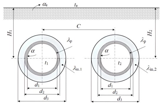
Figure 1.
Geometry of the pipes.
The heat losses required for the creation of a similarity model were identified by applying the balance method. Temperatures at the system’s inlet and outlet were measured using an MI9060 device. The measurement accuracy was ±0.01 °C in a temperature range from −200 °C to +850 °C, with 0.001 °C resolution. A volumetric flow rate of the water was measured, using an ultrasonic flow rate meter with an accuracy of ±0.3% of the measured value.
For the DN65 heat network, the measurements were carried out at three different ambient temperatures: te = 7.5, 10 and 15 °C. As for the DN100 network, the ambient temperatures were: 5, 9 and 13 °C. At each temperature te, 36 measurements were carried out. For the purpose of further analysis, the values of the parameters obtained from a total of 216 measurements were available. Outliers were removed from the set of calculated values for ql. Therefore, when deriving the parameters of a criterial equation, two measurements on the DN65 network and three measurements on the DN100 network were not taken into account.
5. Identification of the Criterial Equation Parameters
The correlation between the dimensionless arguments in Equation (23) is a power function, so the following equations hold:
In logarithmic coordinates, this correlation is linear, as follows:
Individual criteria π were calculated from the measured values of all the quantities. A constant C and the searched exponents z1 to z7 were identified from the results of the experiment by applying a multiple linear regression. The values of the constant C and the exponents z1 to z7 are listed in Table 2.
Table 2.
Constant C and individual exponents.
An analysis of the results indicated that the model was statistically significant. In order to verify the multicollinearity, we applied the Variance Inflation Factor (VIF) quotient. Since the VIF value lied between 1 and 5, the considered criteria did not correlate with the other criteria. Heteroscedasticity was verified using the Breusch-Pagan test. The results indicated that the regression model did not prove the heteroscedasticity. The tests were carried out using the R package software.
For the analysed twin pipe directly-buried heat network, the full criterial Equation (24) was as follows:
6. Discussion and Conclusions
The exponents in Equation (26) indicated that specific heat loss is most affected by the temperature criteria π2 and π1 and by the simplexes π5 and π6. A significantly weaker effect of the other criteria—π3, π4 and π7—may be explained after a more detailed analysis of the process of heat transfer from hot water to the surrounding environment. A sensitivity analysis of the individual thermal resistances indicated a weak effect of the quantities that are present in those criteria—H, C and αe—on the heat loss value. Moreover, the effect of the quantity H was most reduced due to the fact that the measurements were carried out on two networks with identical pipe burial depths.
The results obtained from the similarity model and the results obtained from the measurements exhibited a very good agreement. Figure 2 shows the correlation between the specific heat loss ql,mea calculated from the results of the measurements and ql,mod calculated using the criterial Equation (26).
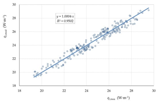
Figure 2.
Correlation between the specific heat losses obtained by the measurements and from the model.
The correlation may be described by a regression line with the slope approaching 1, in particular 1.0004, with the coefficient of determination (square power of the correlation coefficient) R2 = 0.9502. The standard deviation of the difference was sΔ = 0.515 W·m−1.
The results of both methodologies were also tested by using a paired t-test at a significance level of p = 0.05. The value of the test criterion t was calculated using the following equation:
where m is the number of values.
The quantity is an average value of the difference ql,mea − ql,mod calculated using the following equation:
For the analysed datasets, m = 211 and W·m−1; therefore, the value of the test criterion was t = 0.492. The critical value tcr at a significance level of 0.05 was t0.05(211-1) = 1.971. Since t < tcr, it may be stated that both of the methodologies led to identical results.
The criterial Equation (26) represents a universal formula for expressing the specific heat loss for a twin pipe directly-buried heat network. The ranges of the quantities to which the derived model applies are listed in Table 3.
Table 3.
Scope of applicability of the created model.
An advantage of defining the specific heat loss using a criterial equation is that it facilitates the identification of specific heat loss, as well as the heat loss of the entire distribution system, without the necessity to perform repeated accurate measurements.
An example of using the model, when the temperature of water in the feed pipe t1 = 81 °C, is shown in Figure 3, comparing the specific heat loss of the DN65 network and that of the DN100 network. The values of the other quantities were as follows: λin = 0.027 W∙m−1∙K−1; te = 5 °C; λs = 1.5 W∙m−1∙K−1; αe = 23 W∙m−2∙K−1; H = 0.97 m. The figure indicates the following:
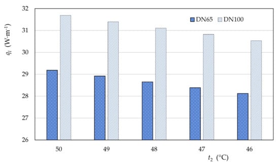
Figure 3.
Comparison of specific heat losses of the DN65 and DN100 networks.
- -
- Heat loss decreased as the temperature of the water in the return pipe decreased;
- -
- The DN100 network exhibited a 2.5 W∙m−1 higher specific heat loss compared to the DN65 network.
The resulting model is primarily intended for the distributors of heat, for the purpose of identifying the specific heat loss, as well as the total dissipation rate of a heat distribution pipeline with a known length of piping. Equation (26) may be programmed in a simple manner to facilitate the identification of the specific heat loss, as well as the total dissipation rate of a heat network. For other ranges of the relevant quantities, it will be necessary to perform another experiment and modify the constant and the exponents in Equation (26).
Author Contributions
Conceptualisation, M.Č. and M.P. (Miroslav Příhoda); Formal analysis, M.Č. and N.J.; Visualisation, T.B. and M.P. (Michal Puškár); Validation, M.P. (Miroslav Příhoda) and M.L. All authors have read and agreed to the published version of the manuscript.
Funding
This paper was written with the financial support from the VEGA granting agency within the Projects No. 1/0224/23 and No. 1/0532/22, from the KEGA granting agency within the Project No. 012TUKE-4/2022, and with the financial support from the APVV granting agency within the Projects No. APVV-15-0202, APVV-20-0205 and APVV-21-0274 and project SP 2023/34-FMT VŠB TUO.
Informed Consent Statement
Informed consents were obtained from all subjects involved in the study.
Conflicts of Interest
The authors declare no conflict of interest.
References
- Čarnogurská, M.; Brestovič, T.; Lázár, M.; Jasminská, N.; Puškár, D.; Příhoda, M.; Marek, J. Measurement of Thermal Conductivity of Sludge and Liquid Materials. In MATEC Web of Conferences; AEaNMiFMaE 2018, EDP Sciences: Les Ulis, France, 2018; Volume 168, pp. 1–6. [Google Scholar]
- Hnizdil, M.; Kominek, J.; Lee, T.-W.; Raudensky, M.; Carnogurská, M.; Chabicovsky, M. Prediction of Leidenfrost Temperature in Spray Cooling for Continuous Casting and Heat Treatment Processes. Metals 2020, 10, 1551. [Google Scholar] [CrossRef]
- Brestovič, T.; Čarnogurská, M.; Příhoda, M.; Lázár, M.; Pyszko, R.; Jasminská, N. A Similarity Model of the Cooling Process of Fluids during Transportation. Processes 2021, 9, 802. [Google Scholar] [CrossRef]
- Hongtao, G.; Fei, M.; Yuchao, S.; Jiaju, H.; Yuying, Y. Effect of adding copper oxide nanoparticles on the mass/heat transfer in falling film absorption. Appl. Therm. Eng. 2020, 181, 115937. [Google Scholar] [CrossRef]
- Davis, B.W.; Pobladov-Ibanez, J.; Sirignano, W.A. Two-phase developing laminar mixing layer at supercritical pressures. Int. J. Heat Mass Transf. 2021, 167, 120687. [Google Scholar] [CrossRef]
- Xiao, H.; Liu, Z.; Liu, W. Turbulent heat transfer enhancement in the mini-channel by enhancing the original flow pattern with v-ribs. J. Heat Mass Transf. 2020, 163, 120378. [Google Scholar] [CrossRef]
- Adachi, T.; Fujita, K.; Nagai, H. Numerical study of temperature oscillation in loop heat pipe. Appl. Therm. Eng. 2019, 163, 114281. [Google Scholar] [CrossRef]
- Živčák, J.; Puškár, M.; Brestovič, T.; Nagyová, A.; Palko, M.; Palko, M.; Krajňáková, M.; Ivanková, J.; Šmajda, N. Development and Application of Advanced Technological Solutions within Construction of Experimental Vehicle. Appl. Sci. 2020, 10, 5348. [Google Scholar] [CrossRef]
- Puškár, M.; Brestovič, T.; Jasminská, N. Numerical simulation and experimental analysis of acoustic wave influences on brake mean effective pressure in thrust-ejector inlet pipe of combustion engine. Int. J. Veh. Des. 2015, 67, 63–76. [Google Scholar] [CrossRef]
- Kleiner, T.; Eder, A.; Rehfeldt, S.; Klein, H. Detailed CFD simulations of pure substance condensation on horizontal annular low finned tubes including a parameter study of the fin slope. Int. J. Heat Mass Transf. 2020, 163, 120363. [Google Scholar] [CrossRef]
- Zhou, Y.; Zhao, C.; Li, K.; Yang, C. Numerical analysis of thermal conductivity effect on thermophoresis of a charged colloidal particle in aqueous media. Int. J. Heat Mass Transf. 2019, 142, 118421. [Google Scholar] [CrossRef]
- Aminu, Y.; Sedat, B. Modelling a Segmented Skutterudite-Based Thermoelectric Generator to Achieve Maximum Conversion Efficiency. Appl. Sci. 2020, 10, 408. [Google Scholar] [CrossRef]
- Nosek, R.; Backa, A.; Ďurčanský, P.; Holubčík, M.; Jandačka, J. Effect of Paper Sludge and Dendromass on Properties of Phytomass Pellets. Appl. Sci. 2021, 11, 65. [Google Scholar] [CrossRef]
- Čarnogurská, M.; Brestovič, T.; Příhoda, M. Modelling of Nitrogen Oxides Formation Applying Dimensional Analysis. Chem. Process Eng. 2011, 32, 175–184. [Google Scholar] [CrossRef]
- Zeleňáková, M.; Čarnogurská, M. A dimensional analysis-based model for the prediction of nitrogen concentrations in Laborec River, Slovakia. Water Environ. J. 2013, 27, 284–291. [Google Scholar] [CrossRef]
- Čarnogurská, M.; Příhoda, M.; Zeleňáková, M.; Lázár, M.; Brestovič, T. Modeling the Profit from Hydropower Plant Energy Generation using Dimensional Analysis. Pol. J. Environ. Stud. 2016, 25, 73–81. [Google Scholar] [CrossRef] [PubMed]
- Rédr, M.; Příhoda, M. Basics of Thermal Engineering; SNTL: Praha, Czech, 1991; pp. 272–294. (In Czech) [Google Scholar]
- Langhar, H.L. Dimensional Analysis and Theory of Models; Robert, E., Ed.; Kreiger Publishing Company: Malabar, FL, USA, 1987. [Google Scholar]
- Barenblatt, G.I. Dimensional Analysis; Gordon and Breach Science Publishers: New York, NY, USA; London, UK; Paris, France; Montreaux, Switzerland; Tokyo, Japan, 1987. [Google Scholar]
- Görtler, H. Dimensionsanalyse: Theorie der Physikalischen Dimensionen mit Anwendungen; Springer: Berlin/Heidelberg, Germany, 1975. [Google Scholar]
- Kožešník, J. Similarity Theory and Modelling; Academia: Praha, Czech, 1983. (In Czech) [Google Scholar]
- Huntley, H.E. Dimensional Analysis; Dover Publications: New York, NY, USA, 1967. [Google Scholar]
- Čarnogurská, M.; Příhoda, M. Application of Dimensional Analysis for Modeling Phenomena in the Field of Energy; SjF TUKE: Košice, Slovak, 2011; pp. 113–129. (In Slovak) [Google Scholar]
- Čarnogurská, M. Basics for Mathematical and Physical Modelling in Fluid Mechanics and Thermomechanics; Vienala: Košice, Slovakia, 2000; pp. 67–98. (In Slovak) [Google Scholar]
- Čarnogurská, M. Dimensional Analysis and Theory of Similarity and Modelling in Practise; SjF TUKE: Košice, Slovak, 1998; pp. 10–56. [Google Scholar]
- Čarnogurská, M.; Příhoda, M. Applied Fluid Mechanics; SjF TUKE: Košice, Slovakia, 2021; pp. 311–420. (In Slovak) [Google Scholar]
Disclaimer/Publisher’s Note: The statements, opinions and data contained in all publications are solely those of the individual author(s) and contributor(s) and not of MDPI and/or the editor(s). MDPI and/or the editor(s) disclaim responsibility for any injury to people or property resulting from any ideas, methods, instructions or products referred to in the content. |
© 2023 by the authors. Licensee MDPI, Basel, Switzerland. This article is an open access article distributed under the terms and conditions of the Creative Commons Attribution (CC BY) license (https://creativecommons.org/licenses/by/4.0/).