Improving Grain Size Analysis to Characterize Sedimentary Processes in a Low-Energy River: A Case Study of the Charente River (Southwest France)

Abstract

The recognition and quantification of fluvial transport and depositional processes has widely been studied. However, few works have focused on the interpretation and quantification of sedimentary processes in low-energy fluvial environments. This paper features and compares the results of five methods of grain size data processing (statistic moments, textural analysis, multivariate statistics combining Principal Component Analysis and hierarchical cluster analysis, and CM image and end-member modeling analysis) and discusses their efficiencies in characterizing low-energy alluvial plain deposits. These environments are characterized by fine grain size, high-homogeneity deposits at the macroscopic scale, and low grain size variability, hence presenting a difficulty in identifying and splitting an apparently homogeneous sedimentary record into sedimentary sequences. These statistical methods are applied on a ~9 m long core extracted from the fluvial island of la Baine located in the downstream section of the Charente River (Chaniers, Charente-Maritime, France). In the light of these results, elementary statistical parameters (statistical moments, modes, and sorting index) have limited interest in the sedimentary description and interpretation of fine fluvial deposits. Textural analyses are more informative but highly dependent on the classification scheme. Only the multivariate statistics approach and end-member modeling analysis present interesting results and allow the robust identification of sub-units. However, multivariate statistics results are dependent on the choice of input variables and do not support non-zero values, while the second method, the most recent and complex one, needs further developments to clearly connect end-member classes to sedimentary processes.

1. Introduction

While the recognition and quantification of fluvial transport and depositional processes have been studied for many years, few works have focused on the description, characterization and interpretation, and quantification of sedimentary processes in low-energy fluvial environments. The study of these environments presents challenges for sedimentological work due to their high degree of homogeneity at the macroscopic scale, low particle size contrast (silt-clay deposits), and the absence of microscale stratigraphic features (laminations). To provide a first insight, this paper discusses the results of five approaches to processing grain size data and evaluates their effectiveness in characterizing low-energy alluvial plain deposits. The question is: to what extent can conventional or more recent grain size processing methods be used to decipher this type of sedimentary record?

This study focuses on and compares the results obtained using five different methods: statistical moments, textural analysis, CM image analysis, multivariate statistics employing successive Principal Component Analysis and Hierarchical Cluster Analysis (Appendix A) on various data sets, and an end-member approach (EMMAgeo). These methods were applied to an approximately 9 m-long core extracted from the fluvial island of la Baine, located downstream of the Charente River near Saintes in Charente-Maritime, France.

2. Literature Review

The grain sizes of natural particles are crucial parameters in various Earth science fields, archaeology, engineering sciences, and life sciences. Grain size is a characteristic of unconsolidated materials that influences their physical and mechanical properties and potential applications and provides information about their origins, deposition processes, or aquatic habitats in both river and ocean contexts. Consequently, it is commonly used in fields such as geomorphology, pedology, geotechnics, geoarchaeology, ecology, and more.

Grain size analysis has long been a preferred method for describing unconsolidated sediments, particularly in studying depositional environments, paleogeography, and depositional processes. The early work by Rivière [1] highlights the benefits and limitations of this approach, which has been applied to various environments such as lakes, deserts, glaciers, oceans, estuaries, and rivers. However, since the late 1970s, the development of facies sedimentology has somewhat diminished the use of grain size methods due to the labor-intensive nature of measurements, which are primarily carried out through densimetry and sieving. Additionally, interpreting the results without a current frame of reference has proven challenging. Apart from Bagnold’s [2] notable contributions, the adoption of this approach has been limited.

Grain size data are inherently complex and difficult to analyze and represent. To simplify analysis, grain size complexities are often reduced to three categorical data: gravel, sand, and mud or sand, silt, and clay, plotted on ternary diagrams. These categories are determined by particle size limits, often expressed in millimeters (mm), micrometers (μm), or phi scale (Ø) units such as the Wentworth or Udden-Wentworth scale, Krumbein Ø scale, etc. While this categorization method is simple and quick, it relies on arbitrary choices for class limits and sub-categories. This becomes even more challenging when dealing with samples of mixed origin [3]. Consequently, finding the most suitable texture classification scheme that maximizes the contrast between samples becomes necessary. The R package Soil Texture Wizard, which utilizes data generated by Gradistat, can be employed for this purpose.

The seminal work of Folk and Ward [3], supplemented by Folk’s later update [4], as well as Passega’s contemporary contributions [5,6], laid the foundation for a rational description of grain size data through statistical analysis. These publications primarily employed elementary statistical approaches, such as the first and second statistical moments (mean, mode, skewness, and kurtosis) [3] or percentiles (e.g., D₅₀ and D₉₉) [5]. However, the theoretical basis for such usage remains weak as these approaches assume a Gaussian lognormal and unimodal sediment distribution, which is rarely the case [7,8]. Semi-quantitative indices like sorting indices (Trask’s index [9], Inman’s index [10], Folk and Ward index [3], etc.) are often temporary solutions and tend to correlate with standard deviation [11]. Nevertheless, despite their limitations, central tendency values (mean, median), shape indices (skewness and kurtosis), and dispersion indices (sorting, etc.) remain dominant in interpreting and graphically representing grain size distributions. The popularity of software like Gradistat [12] and its successive updates (currently version 9.1) attests to this.

These approaches are still valuable for identifying trends, gradients, discontinuities, or depositional events in the sedimentary record. Some authors, such as Stewart [13], have attempted to combine statistical values, particularly standard deviation and asymmetry, to identify depositional environments. Moiola and Weiser [14] focused on the variance–asymmetry relationship to characterize beach environments. These methods remain popular in the study of transitional environments despite their lack of theoretical foundation.

Sly [15] proposed a similar approach for distinguishing beach deposits. Passega [5,6] worked along the same lines by developing the CM image and identifying depositional processes based on the median (D₅₀) and extreme (D₉₉) grain sizes. He divided the resulting graph into homogeneous segments (R-S, S-T, etc.) associated with depositional processes such as traction, homogeneous suspension, graded suspension, and decantation. Once again, addressing the complexity of particle size distribution involves reducing it to one or two indices without considering the biases related to the statistical distribution, particularly the significance of the mean in a multimodal sample.

Visher [16] proposed a different approach that focuses on utilizing the entire curve rather than reducing it to a series of indices or notable points through the segmentation of cumulative frequency in lognormal coordinates. Mercier [8] proposed an improvement and a geomorphological interpretation of this approach. Since the late 1970s, the development of computerized data processing methods, especially multivariate analysis, has offered an alternative for processed grain size data. This was briefly mentioned by Rivière [1] and implemented by Syvitski [17] among others. However, this type of approach remains underutilized [18,19,20,21]. The optimization of this treatment, particularly in the selection of descriptive variables to be included in multivariate analysis, is seldom discussed. An alternative to statistical approaches is decomposition based on mixing laws. Several authors [22,23,24] have demonstrated that particle size curves of many samples correspond to mixtures of lognormal sub-samples. It is then possible to propose the decomposition of entire curves into the sums of lognormal functions, wherein the means, modes, and standard deviations serve as relevant data. Several software tools that are not specific to sedimentology can be used for this purpose, such as PeakFit^® or the R package MixTools among others. More recently, Dietze et al. [25,26,27] have developed a statistical approach to decompose multimodal grain size samples into their end-member contributions using R’s package EMMAgeo. Until now, this approach has been limited to a few case studies [28,29,30,31,32,33] and remains underutilized in sedimentology. Its effectiveness needs to be demonstrated through concrete examples in fluvial sedimentology. Although EMMA is a robust and reliable tool for identifying and quantifying sediment processes, the algorithm may underestimate contributions from low end-members and overestimate high contributions [27].

3. Study Area

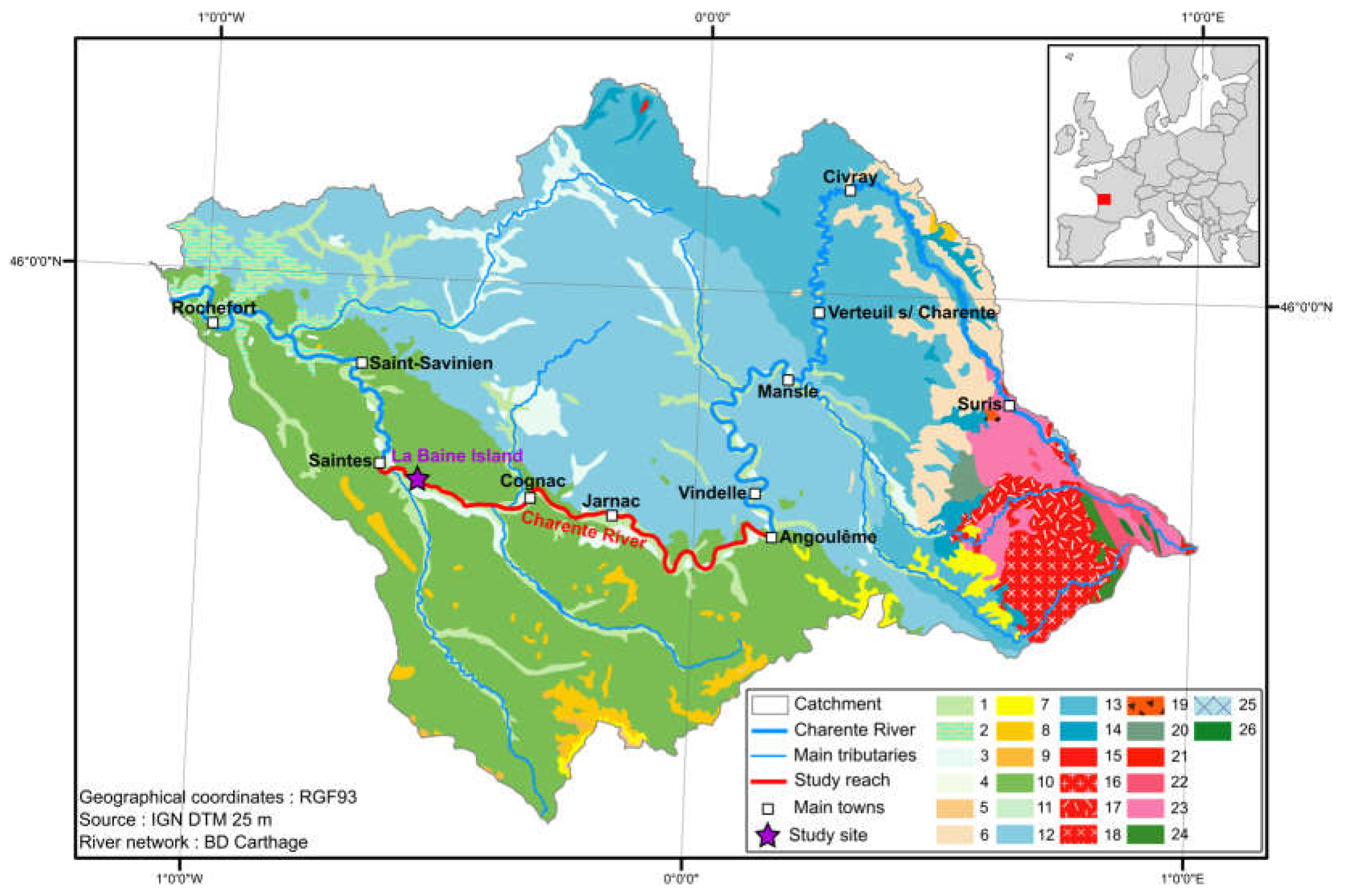
Located on the Atlantic coast in southwest France, the Charente River exhibits specific characteristics. It has a low gradient of 0.00086 m.m⁻¹ and low energy with an approximate value of 10 W.m⁻² (Figure 1). The river has a drainage basin of around 10,550 km² and stretches for approximately 365 km from its source in Chéronnac to its estuary. The fluvial pattern of the Charente River undergoes changes along its course. It starts as an irregular incised single channel from its source to Civray, transitions to a highly anastomosed pattern with 2–13 channels between Civray and Angoulême, becomes discontinuous and weakly anastomosed with 3–5 channels from Angoulême to Cognac, and finally takes on a meandering-to-sinuous single-channel form from Cognac to the estuary [34,35,36,37].

The catchment area of the Charente River consists of different geological formations. In the upstream section, it is composed of metamorphic and granitic complexes from the Massif Central. North of a line connecting Angoulême and Rochefort, the catchment is characterized by monoclinal Jurassic limestone. South of this line, there are folded anticline-syncline structures within Cretaceous sandy-clay detritic deposits. These deposits are overlapped by Holocene fluvio-marine deposits in the downstream part of the catchment [38,39].

The catchment area of the Charente River experiences a temperate oceanic climate classified as Cfb in the Köppen climate classification system. It is characterized by cool winters, with an average temperature of 6 °C in January, and moderately warm summers, with an average temperature of 20 °C in July. The annual temperature range is relatively low, at around 14 °C, and the average annual rainfall is close to 800 mm. However, the average annual precipitation within the catchment varies between 700 mm and over 1000 mm depending on the north–south gradient and altitude [40].

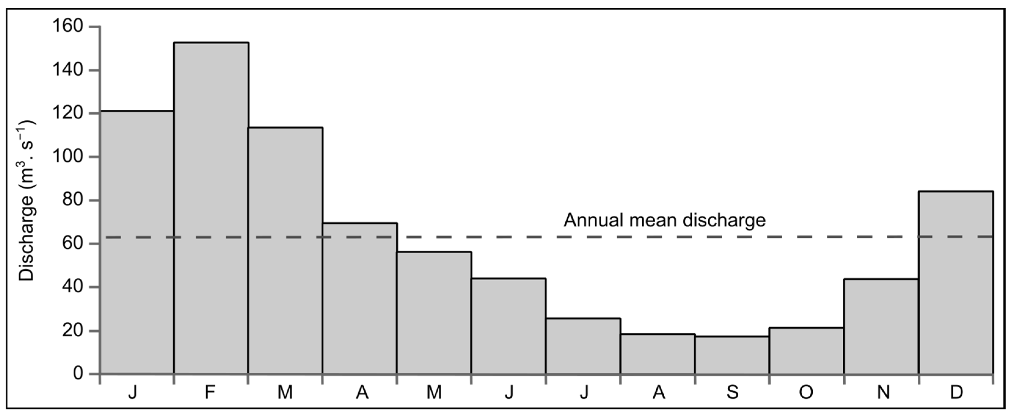
The flow regime of the Charente River can be described based on data from the Chaniers gauging station, which is in the downstream part of the study area (Figure 2). It exhibits characteristics typical of Atlantic lowland rivers, following a rain–evaporation regime. The river experiences dominant winter floods, which are associated with prolonged and intense precipitation resulting from westerly depressions. These winter floods mainly occur between December and February [41]. Additionally, there are fall and spring floods caused by short but intense rainfall events following wet seasons in summer or winter. Throughout the year, the Charente River goes through a high-water stage from December to March and a low-water stage from July to October. The highest monthly mean discharge, reaching 152 m³.s⁻¹, is observed in February, while the lowest monthly mean discharge, around 16.9 m³.s⁻¹, is recorded in September. The annual mean discharge is 62.9 m³.s⁻¹. Notably, a minimum daily discharge of approximately 9 m³.s⁻¹ was recorded in September 2020, while a maximum daily discharge of 550 m³.s⁻¹ (equivalent to Q20) was noted on 8 February 2021. Within the study area (Figure 1), the Charente River does not have any major tributaries and is considered hydrologically homogeneous.

Above the Chaniers gauging station, the Charente River exhibits very low stream power, which is estimated to be around 5 W.m⁻². This is primarily due to the presence of a moderate bankfull discharge, approximately 200 m³.s⁻¹, and a gentle slope of around 0.0002 m.m⁻¹ [35]. According to the classification by Nanson and Croke [42], the Charente River falls under the category of low- or very-low-energy rivers, with stream powers greater than 10 W.m⁻². Consequently, its capacity for sediment transport and adjustment is limited. Currently, there is a lack of solid transport data for the Charente River between Angoulême and Saintes, with only a few data points available for the estuary. In the estuary, it has been estimated that the Charente River transports approximately 78,000 tonnes of sediment per year, resulting in a low erosion rate of around 0.4 mm.year⁻¹ [43].

Field observations within the study area indicate a predominant fine suspended load and a limited bedload consisting mainly of sandy sediments, particularly upstream from Cognac. Duquesne et al. [34,35] have shown that fluvial forms have very limited mobility in the medium term (around 150 years) due to the natural characteristics of the river such as its very low slope and flood flows with minimal morphogenic effects. Additionally, there is minimal change in the number of islands, except for those influenced by human activities [36].

The focus of this study is the section between Angoulême and Saintes, spanning approximately 100 km in length. This reach of the Charente River is characterized by a significant change in its fluvial pattern near Cognac [34,35]. Upstream from Cognac, the river exhibits a discontinuous and weakly anastomosed pattern, with an average stream power of 10 W.m⁻² and an average gradient of around 0.0002 m.m⁻¹. These values classify this section of the river as an “anastomosed river, organic flood plains type C2a” according to the classification by Nanson and Croke [42]. The landscape is characterized by a network of interconnected channels (2–5 channels), which are separated by large, elongated, and vegetated islands [36]. The width of the alluvial plain ranges from 1 to 2 km. The channels have a low sinuosity (approximately 1.05) and moderate width–depth ratios (around 15) and are bordered by natural low levees [34,35].

The downstream section, from Cognac to Saintes, is primarily characterized by a predominant sinuous-to-meandering single channel. The channel is confined within a narrower alluvial plain with a width ranging from 0.5 to 1.5 km, and evidence of side channel changes is relatively scarce [34]. The channel width in this single-channel section ranges from 30 to 70 m, with a mean width–depth ratio of approximately 10 [35]. The mean stream power in this segment is estimated to be around 7 W.m⁻², and the average low-gradient is approximately 0.0001 m.m⁻¹. This segment can be classified as “Laterally stable single channel floodplains type C1” according to the classification system by Nanson and Croke [42].

The coring site, located on la Baine Island, is positioned in the downstream section of the Charente River near the village of Chaniers. It is situated approximately 15 km upstream of Saintes (Figure 1). The site exhibits a multi-channel pattern with vegetated islands of varying sizes, morphologies, and ages. This section of the river is characterized by meandering channels. The altitude at the site is relatively low, with an average elevation of 4 m above sea level. The dominant land use in the area is agriculture, including arable farming and grassland.

Historical records indicate significant hydraulic engineering activities carried out during the 19th century to enhance river navigation. These works included the construction of locks, embankments, canals, and dams. Additionally, the water flow was utilized to power wheat mills, water mills, and weirs, with evidence of such structures dating back to the 14th century. The history of engineering interventions for navigation and water mills over the past three centuries is summarized in the work by Duquesne [35].

4. Materials and Methods

4.1. Core Data Acquisition

Three cores, with depths ranging from 6 m to 9 m, were obtained from the alluvial plain as shown in Figure 3 (refer to

Table 1. Information on the cores performed on la Baine Island site. Geographical coordinates are expressed in Lambert-93. The core in bold is the core studied in this paper.

Core	Longitude	Latitude	Altitude	Depth (m)
CHA01	424208.4	6518230.9	4.24	9
COU01	423622.4	6518814.5	4	9
COU02	423300.3	6518442.0	3.25	6

for detailed information). Although the three cores exhibit similar characteristics, this paper focuses on the longest core, CHA01, which reaches a depth of 9 m. CHA01 is situated in the southeastern part of la Baine Island, close to an abandoned navigation channel that served as a detour for navigating obstacles (Figure 3). Once extracted, the core was initially split, photographed, and described based on macroscopic texture, sedimentary structures, and the presence of macro-remains.

4.2. Chronology

The chronology of core CHA01 was established using AMS radiocarbon dating conducted on plant remains or organic sediments, as outlined in

Table 2. ¹⁴C dating of the core CHA01.

Depth (cm)	Laboratory Code	Material	14C Age B.P.	Age cal. B.P. (2σ)
485	ULA-8845	Plant remain	5080 ± 20	5749–5829 (64.1) 5847–5904 (30.7)
553	ULA-8846	Plant remain	5175 ± 20	5904–5944 (67.6) 5965–5991 (27.3)
617	ULA-9257	Plant remain	5865 ± 15	6652–6739
734	ULA-9254	Plant remain	6180 ± 15	7001–7134 (89.1) 7149–7160 (5.7)
810	ULA-8848	Plant remain	6220 ± 25	7009–7130 (66.5) 7151–7170 (11.4) 7206–7247 (16.9)
880	ULA-539073	Organic material	6920 ± 30	7677–7795 (88) 7811–7832 (6.9)

. Radiocarbon dates obtained were then calibrated using the R package CLAM and the Intcal20.14C radiocarbon calibration curve [44,45]. The radiocarbon ages were calculated with a 95% confidence range (two sigmas) and expressed as calibrated years before present (cal. years B.P.).

A deterministic age–depth model was generated (Figure 4), covering the period since the early Atlantic. The base of core CHA01 was estimated to be around 7915 cal. years B.P. However, it should be noted that the top section of the core (the last 4 m) lacks radiocarbon dating and alternative dating methods. Therefore, the age–depth model for the uppermost part of the core should be interpreted cautiously due to this limitation.

4.3. Grain Size Analysis

A total of 158 sediment samples were collected at 5 cm intervals for grain size analysis. A constant volume of 2 cm³ was retrieved from each sample for further analysis. The collected sediment samples were subjected to oven drying at 105 °C for 24 h. Subsequently, 5 g of sediment were treated with a sodium hexametaphosphate solution at a concentration of 180 g/L to disperse any aggregates present. Grain size analysis was conducted using a Horiba LA-960V2 laser particle size analyzer. The obtained data represent the volume percentage of each grain class; they were classified into 97 different grain size classes ranging from 0.01 to 3000 mm.

4.4. Elementary Statistical Parameters

The grain size data were initially processed using the Gradistat software for standard statistical analysis [12]. This involved extracting basic statistical parameters such as sorting, skewness, and kurtosis [3]. The method of moments [46,47] is commonly used to describe grain size distributions [48]. However, it is important to note that these parameters can be highly influenced by outliers located in the tails of the distribution [49] and mixing processes. Other commonly used statistical descriptors include the mean, median, and mode(s) [48]. The mean and median are relatively easy to compute but may not always be reliable. The mean is heavily influenced by extreme values in the distribution’s tails, while the median does not adequately account for extreme values [49]. Therefore, caution must be exercised when interpreting these statistical parameters. The primary mode is the most appropriate descriptor for unimodal samples [12], but it may not necessarily correlate with the transport power in the case of multimodal grain size distributions. Although the Gradistat software calculates primary, secondary, and ternary modes, only the first main mode was retained for sample description and the multivariate statistical approach (PCA and HCA).

4.5. Textural Analysis

Fine grain size classes are often categorized as sand, silt, and clay or a combination of these terms [50]. However, the splitting of mixed samples into categorical nomenclature remains a topic of discussion because the limit values between these categories are somewhat arbitrary and can be described using either metric or phi scales [51]. The choice of textural classification scheme used is crucial for interpreting the results. To represent these data, a textural triangular analysis is a simple approach. In this study, the sand–silt–clay content was determined using the Gradistat software [12] following Folk’s classification system [52]. The textural data were then processed using the R package Soil Texture Wizard, developed by Moeys [53]. The Soil Texture Wizard package generates texture triangles and applies various texture classification schemes. In this case, five texture classification systems were selected: that of the US Department of Agriculture (USDA TT) [54], the European Soil Map (HYPRES) [55], and those of the UK Soil Survey of England and Wales (UK SSEW) [56], French “Aisne” [57,58], and International Soil Science Society (ISSS) [59]. To compare the sensitivities of these classifications, each resulting qualitative class was assigned a value ranging from 1 to 5 or 1 to 11, depending on the class number proposed by the classification scheme. This coding system allowed for graphical representation and facilitated the comparison of the different classification schemes.

4.6. Multivariate Statistical Analysis

Principal Component Analysis (PCA) is a set of methods used to analyze complex data [60,61,62,63]. It is an exploratory or descriptive technique commonly applied to quantitative data. In the context of grain size analysis, the data set consists of individuals (samples) and properties (such as grain size classes or index values). To assess the usefulness of PCA in grain size analysis, we conducted tests on three types of data sets that have been used in previous publications. In the first data set, we considered only four properties: mode, sorting index, kurtosis, and skewness, as proposed by Simon et al. [21]. The second data set included six properties: mode, sorting index, kurtosis, skewness, and sand–silt–clay proportions. These additional values are considered important in low-energy fluvial contexts. Lastly, we performed a test on raw grain size data, including 77 non-zero grain size classes ranging from 0.1 mm to 3000 mm. To group the individuals (samples) into clusters based on their characteristics, we applied Hierarchical Cluster Analysis (HCA) to the three sets of PCA scores. The main objective of HCA is to create clusters that minimize the variability of samples within each cluster while maximizing the variability between clusters [61]. To perform this analysis, we utilized the R package Cluster, which applies an algorithm developed by Kaufman and Rousseeuw [64]. The Euclidean distance and Ward’s method [65] were employed as measures of similarity between observations, and an agglomerative method was used to combine clusters.

4.7. CM Diagram

The 50th (D₅₀) or median and the 99th (D₉₉) percentiles of each sample were directly extracted from the Horiba software. A bi-logarithmic plot, called a CM diagram, was built with D₅₀ on the X-axis and D₉₉ on the Y-axis according to the method described by Passega [5,6]. In a CM diagram, the samples tend to cluster in a set of segments that are interpreted as transport/deposition processes. Three major types of sediment transport were distinguished: (1) the rolling of coarse cobbles, pebbles, or sands on the alluvial floor, associated with the NO segment; (2) the saltation of medium and fine sands or graded suspension close to the channel floor on the PQ–QR segment, and (3) the uniform suspension of fine sand, silts, and clay in the water column corresponding to the RS segment. As previously noticed by Bravard and Peiry [66] and Arnaud-Fassetta et al. [67], the position of each segment is relative and specific to each river.

4.8. End-Member Modeling Analysis

End-Member Modeling Analysis (EMMA) has been widely employed in various fields of geoscience. In hydrology, EMMA has been used to identify the sources and flow paths of stormflow in small catchments [68], quantify phosphorus retention and release in rivers [69], determine nitrate concentrations in water flow paths [70], and quantify nutrient dynamics and biological carbon uptake in estuarine zones [71]. In sedimentology, EMMA serves as a statistical approach to identify and quantify sediment transport and deposition processes for sediment samples with multimodal particle size distributions. While EMMA has been applied in marine, lake, and eolian environments, its potential in recognizing transport and deposition processes in low-energy alluvial plains with seemingly sedimentary homogeneity remains unexplored.

The data set (X) used in EMMA consists of sediment samples described by m grain size distributions and n grain size classes. EMMA generates a modeled data set that represents the linear combination of end-member loadings (individual grain size distributions) and end-member scores (the contribution of each loading to each sample) [25,28]. The principles and procedures of the EMMA algorithm have been detailed in previous works [72,73]. For this study, the data set comprised 158 samples described by 69 grain size classes after removing classes with zero values. The grain size data were processed using the R package EMMAgeo [25,26] with an extended protocol to parameterize all steps of robust EMMA. In this analysis, a five-end-member mode was selected based on the samples’ pre-processing.

5. Results

5.1. Elementary Statistical Parameters

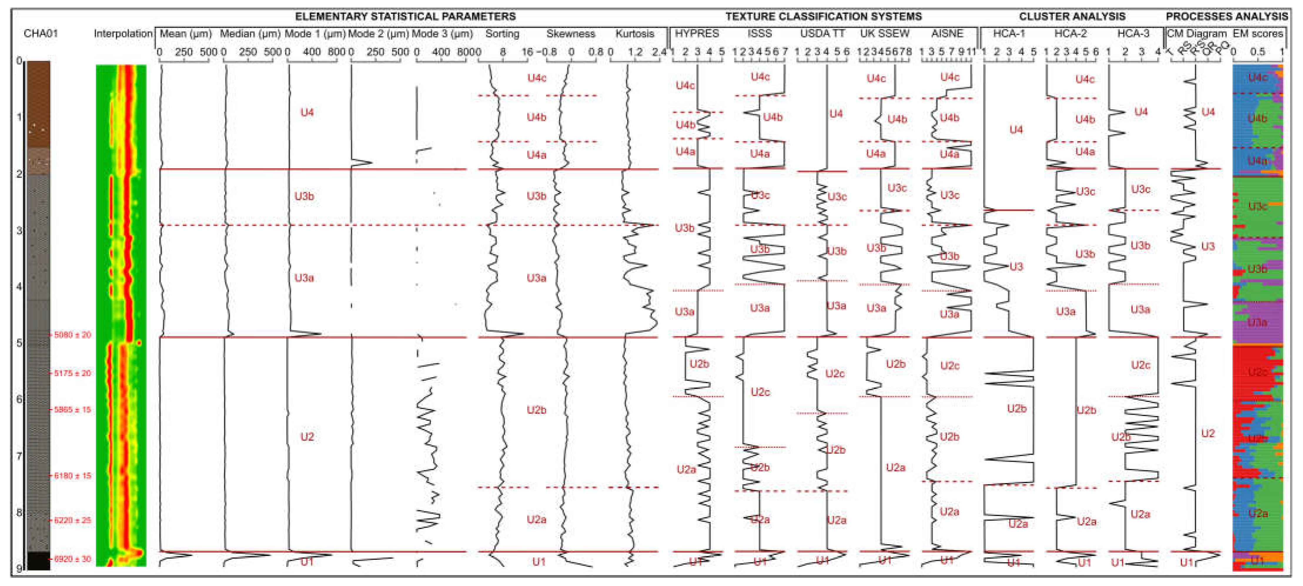
The mean, median, and modal grain sizes of the samples are reported as 15.6 μm, 22.8 μm, and 33 μm, respectively (Figure 5). These values indicate a general trend of fining-up in the grain sizes. The grain size distributions exhibit relatively similar patterns with negative skewness, indicating an asymmetry towards the finer fractions. The kurtosis values suggest a generally platykurtic distribution, indicating a flatter shape compared to a normal distribution. There is also a notable presence of bimodality or trimodality in the grain size distributions, with only a few samples showing unimodal distributions. Based on the vertical variation of these grain size metrics, core CHA01 can be divided into four main stratigraphic units.

Unit 1 (900–869 cm): This unit is dominated by sand (very fine-to-medium) but exhibits high variability. It is a coarsening-up sequence, with the upper part showing the highest mean, median, and mode values (ranging from 64.7 to 332.2 μm, 76.6 to 474.4 μm, and 108.8 to 727.8 μm, respectively), and the lower part having minimal values (ranging from 1.4 to 5.8 μm, 0.5 to 8.2 μm, and 0.4 to 6.3 μm, respectively). Sorting is poor, and skewness and kurtosis show variability, ranging from 0.5 to 0.7 and 0.7 to 1.1, respectively.

Unit 2 (868 cm–488 cm): This unit has the lowest grain size values and a high clay content compared to other units. The mean, median, and mode range from 2.4 to 11.9 μm, 3.2 to 18.6 μm, and 0.3 to 24.5 μm, respectively. Grain size distributions in this unit exhibit high sorting values (ranging from 5.3 to 9.3) and low negative skewness values (ranging from −0.37 to −0.06). Sorting and skewness show increasing trends from the base to 6.90 m. The samples in this unit are multimodal, and kurtosis is very platykurtic, ranging from 0.6 to 1.1.

Unit 3 (487–189 cm): This unit consists of varying degrees of silt and shows a fining-up trend. It can be further divided into two sub-units. Sub-unit 3a (487–290 cm) exhibits the highest mean, median, and modal size values (ranging from 5.5 to 51.7 μm, 10.9 to 108.5 μm, and 21.4 to 534.8 μm, respectively). The sand content remains low (<20%), and the samples are unimodal with highly variable kurtosis values (ranging from platykurtic, 0.6, to 2.3). Sub-unit 3b (289–189 cm) is characterized by increases in silt and clay content, reaching 40% and 50%, respectively. The mean, median, and mode values are lower (ranging from 5.2 to 13 μm, 10.7 to 24.9 μm, and 21.4 to 32.1 μm, respectively). The particle size profiles of the samples in this sub-unit are quite similar, with very low negative skewness (−0.6 to −0.3), dominant bimodality, and a generally platykurtic kurtosis value (ranging from 0.5 to 1).

Unit 4 (188–0 cm): This unit is composed of medium-to-coarse silt but exhibits an enrichment of fine sands by close to 20%. The mean, median, and modal sizes range from 8.1 to 36.5 μm, 28 to 48.2 μm, and 14.1 to 40.4 μm, respectively. Grain size distributions in this unit indicate a similar pattern with low-to-very low negative values.

The analysis of first-order statistical moments (mean, median, and modes) and second-order statistical moments (kurtosis and skewness) suggests that the CHA01 core represents a predominantly homogeneous silty sequence. However, the limitations of these descriptors become apparent in very homogeneous alluvial contexts. While these descriptors provide information about the grain size distribution, they do not provide insights into the sedimentary environment or facilitate interpretation.

It is worth noting that the use of the D₉₀ percentile, as proposed by Duquesne [35], does not offer improvement in the subdivision of the core into different stratigraphic units. This implies that relying solely on percentile values may not be sufficient to characterize the sedimentary variability within the core.

5.2. Textural Triangles

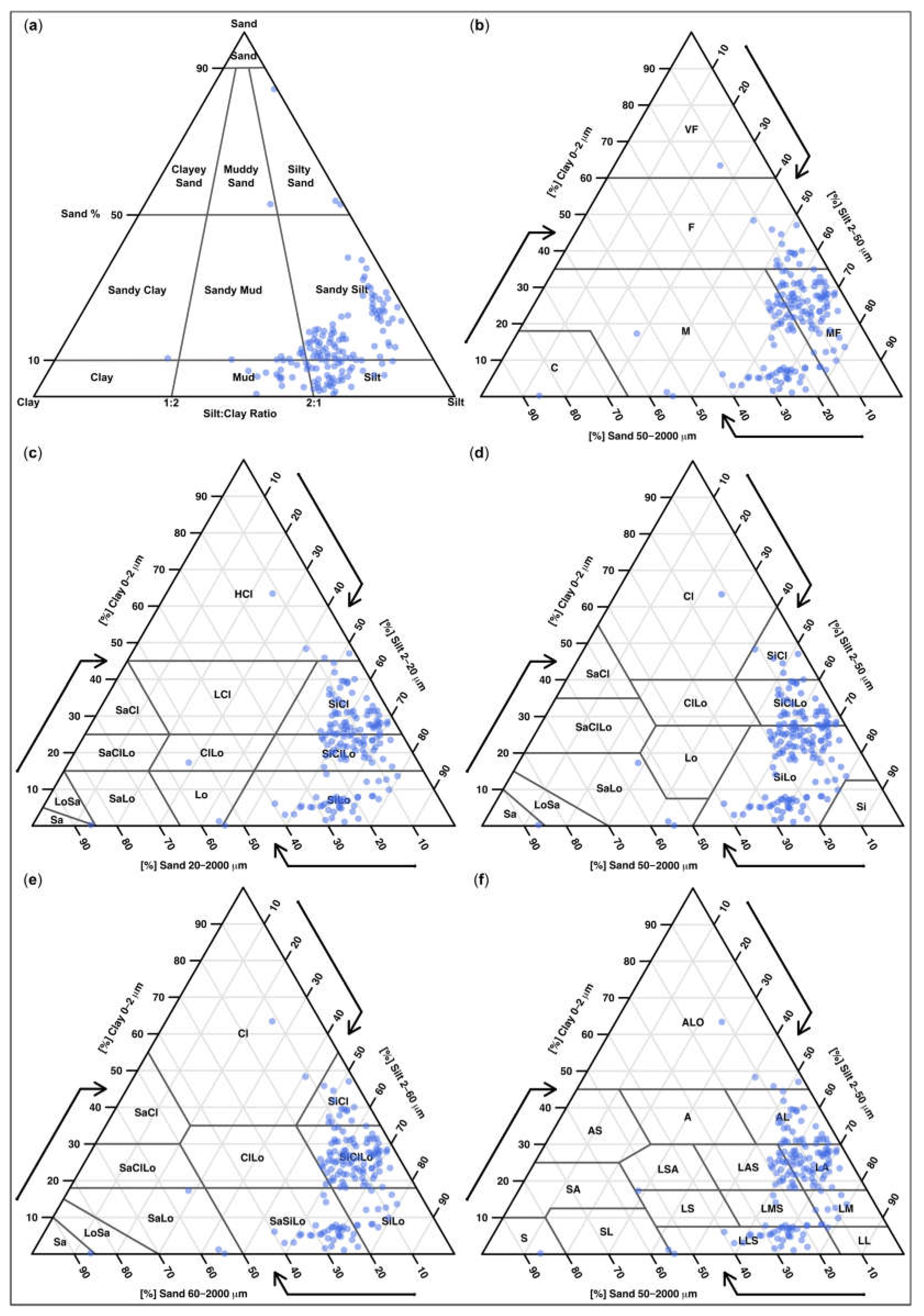
Textural analysis, which involves determining the relative proportions of sand, silt, and clay, is a commonly used method to represent grain size data. However, there is no consensus regarding the boundaries between different grain size categories and sub-categories. To identify the most suitable classification scheme that maximizes the contrast between the samples, six textural classifications were tested on the 158 samples. The resulting membership in each class was encoded to assess the sensitivity of each system and enable a comparison between them (Figure 5).

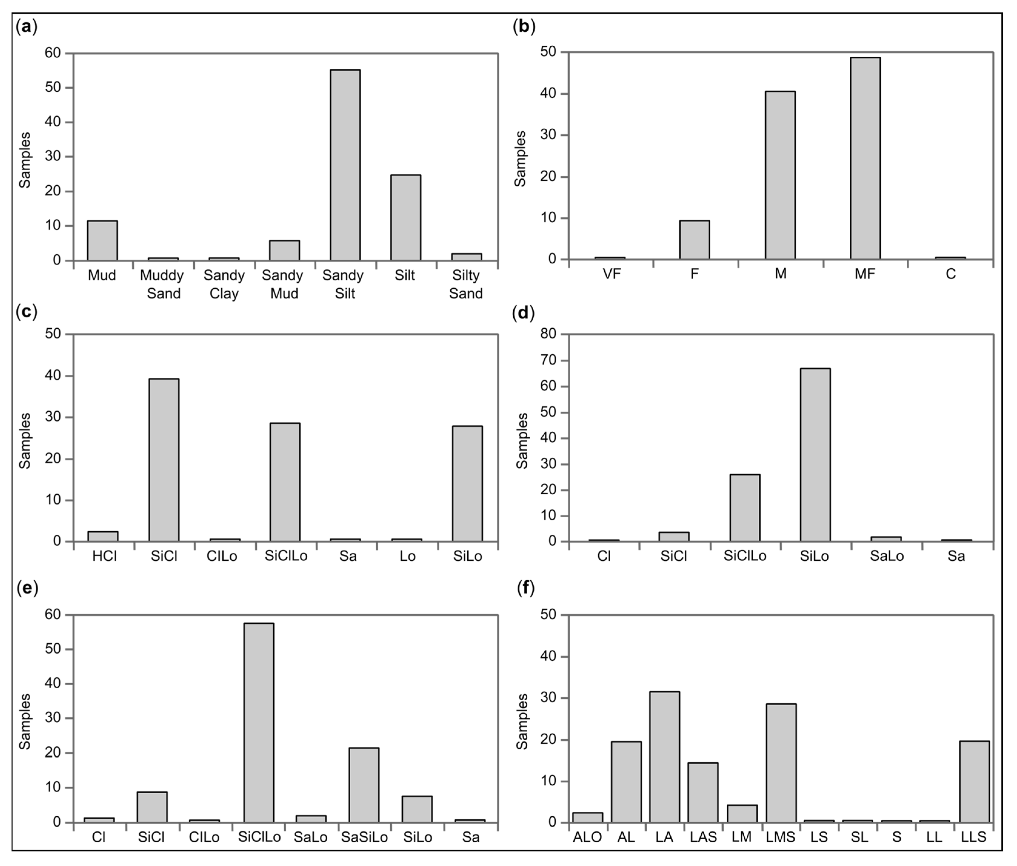
The Folk scheme divides sand–silt–clay samples into 10 sub-categories (Figure 6). For the samples from core CHA01, only seven sub-categories are present, and three of them include only a limited number of samples (one to three individuals). Among the remaining four categories, sandy silt and silts dominate, accounting for 55% and 25%, respectively (Figure 7), while mud and sandy mud are poorly represented (less than 11% and 6%, respectively). This classification scheme was not used to propose a division of the core.

The European soil map (HYPRES) proposes a classification system with only five sub-categories (Figure 6). All of them are represented in core CHA01, but the extreme sub-categories (very fine and coarse) have only one individual each and are of limited usefulness. The remaining three sub-categories are medium-fine (49%), medium (41%), and fine (9%) (Figure 7).

According to the HYPRES sub-categories, the core can be divided into four main units (Figure 5). U1 (900–869 cm) appears highly heterogeneous, encompassing a mixture of all sub-categories. Most of U2 (868–488 cm) is predominantly composed of an alternation between sub-categories 3 and 4 (U2a, 868–594 cm), except for its upper section, which displays a combination of sub-categories 2 and 4 (U2b, 593–488 cm). U3 (487–189 cm) exhibits a composition similar to U2a, except in its base. Consequently, U3 can be further divided into U3a (487–189 cm) and U3b (405–189 cm). U4 represents the most homogeneous unit and is dominated by sub-category 3. However, the presence of sub-category 2 in its middle portion (U4b, 136–90 cm) leads to its subdivision into three sub-units.

Additionally, the ISSS texture triangle provides a 12-sub-category classification system. Among these, only seven are represented in core CHA01, with the top three accounting for 96% of the samples, namely silty clay, silty clay loam, and silt loam (Figure 7).

According to the ISSS classification scheme, the core can also be subdivided into four main units (Figure 5). U1 (900–869 cm) exhibits some fluctuations in sample classification. U2 (868–488 cm) can be divided into three sub-units. The upper sub-unit (868–761 cm) predominantly consists of silty clay loam samples, the middle sub-unit (760–682 cm) varies between containing silty clay and silty clay loam samples, and the lower sub-unit (681–488 cm) primarily comprises silty clay samples. U3 (487–189 cm) can also be divided into three sub-units. U3a (487–394 cm) is composed of silt loam samples, U3b (393–290 cm) exhibits variations between silty clay, silty clay loam, and silt loam samples, and U3c (289–189 cm) consists predominantly of silty clay loam. U4 (188–0 cm) represents a globally homogeneous unit dominated by sub-category 7. However, the presence of sub-category 4 in its middle section (U4b, 141–60 cm) implies in its division into three sub-units.

The USDA Texture Triangle classifies sediments into 12 sub-categories. However, on core CHA01, only seven of these sub-categories are represented, with the top two accounting for over 93% of the samples. The predominant groups are silt loam (67%) and silty clay loam (26%), while silty clay represents a smaller proportion (less than 4%). The remaining sediment categories consist of groups with less than four samples each (Figure 7).

According to this classification scheme, the core can be subdivided into four main units (Figure 5). The lower unit, U1 (900–869 cm), exhibits a mixture of sub-categories but is predominantly composed of silt and sand. U2 (868–488 cm) represents a fining-up sequence that can be further divided into three sub-units. U2a (868–761 cm) exclusively includes silty silt samples. U2b (760–624 cm) is a more heterogeneous mixture of silty clay and silty silt samples. U2c (623–488 cm) consists of silty clay loam interbedded with silty clay samples. U3 (487–195 cm) comprises solely silty silts and silty clays, with the proportion increasing from the bottom to the top. Based on this content, U3 has been divided into three sub-units: U3a (487–389 cm), U3b (388–290 cm), and U3c (289–195 cm). The top of the sequence, according to the USDA scheme, is highly homogeneous, and U4 (194–0 cm) solely contains silty silt samples.

The UK Soil Survey of England and Wales proposes a classification scheme with 11 sub-categories that differs from the previous scheme, particularly in the classification of silty sediments. In core CHA01, the samples are primarily categorized as sandy loam (58%) and silty clay (22%). The dominance of the sandy loam category is surprising considering the relatively low sand content in core CHA01. The other sub-categories each make up less than 5% of the samples, except for sub-categories 2 and 7, which contain only a few samples each.

Similar to the previous schemes, the core CHA01 can be divided into four units (Figure 5). U1 (900–869 cm) is dominated by sands and represents the most heterogeneous unit. U2 (868–488 cm) is predominantly composed of silty clay loam and can be split into two sub-units. U2a (868–594 cm) consists almost entirely of silty clay loam samples, while U2b (593–488 cm) includes interbedded levels of silty clay and silty clay loam. U3 (487–189 cm) exhibits sandy clay and silty textures in varying proportions, allowing it to be further divided into three sub-units: U3a (487–394 cm) mainly contains sandy silt and silty silt samples, U3b (393–264 cm) shows alternating layers of silty clay and silty silt, and U3c (263–189 cm) comprises solely silty clay loam samples. U4 (188–0 cm) consists of sandy-clay loams, with the exception of the intermediate level U4b (141–65 cm), which also contains silty-clay loams.

The Aisne Texture Triangle proposes a division of sand-silt-clay samples into 15 sub-categories (Figure 6). In core CHA01, 11 of these sub-categories are represented. Compared to other classification schemes, the Aisne scheme optimizes the dispersion of clay and silt samples. Four sub-categories encompass more than 85% of the samples: clayey silt (32%), silty clay (20%), sandy silt (20%), and sandy clayey silt (15%) (Figure 7).

According to the Aisne classification scheme, the core CHA01 can be divided into four major units (Figure 5). As in other classifications, U1 (900–869 cm) exhibits a highly variable textural association, dominated by silt and sand. U2 (868–488 cm) is heterolithic and composed of alternating layers of silty clay, clayey silt, and sandy clayey silt. Based on the relative proportions of these sub-categories, U2 has been further divided into three sub-units: U2a (868–744 cm) shows slight alternations of clay silt and sandy clay silt samples, U2b (743–594 cm) exhibits the greatest variability (silty clay, clayey silt, and sandy clayey silt), and U2c (593–488 cm) is primarily composed of silty clay and clay samples. U3 (487–189 cm) is a complex unit that can be subdivided into an almost fine sandy silt (U3a, 487–406 cm), a heterogeneous clayed silt level (U3b, 405–290 cm), and a sub-unit transitioning from silty clay to clay silt (U3c, 289–189 cm). U4 (188–0 cm) can be distinguished into three sub-units. U4a (188–142 cm) consists mainly of fine sandy silt, U4b (141–65 cm) varies between clayey silt and sandy clayey silt samples, and U4c (64–0 cm) comprises fine sandy silt with some medium sandy silt samples.

5.3. PCA and HCA Results

5.3.1. PCA-1 Results

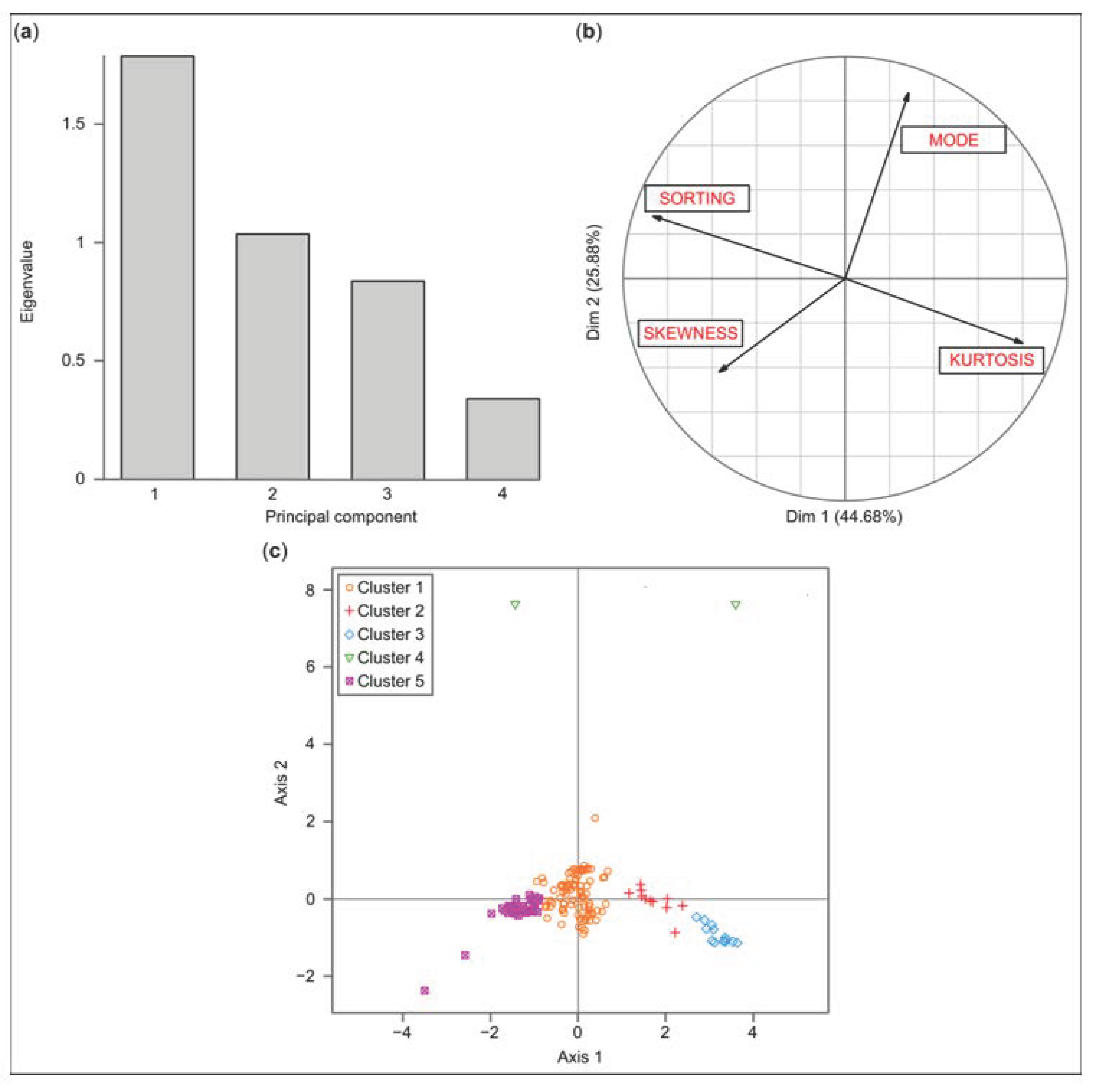
The initial Principal Component Analysis (PCA) was conducted on a limited set of properties, including both the first (mode) and second-order statistical moments (skewness and kurtosis) as well as the sorting index (

Table 3. Correlation matrix of four elementary statistical parameters.

	Mode	Sorting	Skewness	Kurtosis
Mode	1
Sorting	−0.03	1
Skewness	−0.18	0.34	1
Kurtosis	0.13	−0.6	−0.13	1

). The correlation matrix revealed mostly weak correlations among the variables, except for a negative correlation between kurtosis and sorting value. Consequently, the variables exhibited weak correlation and redundancy. The first two PCs account for approximately 71% of the total variance, with PC1 representing 44.68% and PC2 representing 25.88% (

Table 4. Total variance of PCA-1.

Principal Component	Eigenvalue	% of Variance	% of Cumulative Variance
1	1.79	44.68	44.68
2	1.04	25.88	70.57
3	0.84	20.94	91.51
4	0.34	8.49	100

). PC1 primarily captures the variation in grain size samples and is predominantly influenced by the mode values. On the other hand, PC2 contrasts sorting and skewness with kurtosis, reflecting the distinction between homogeneous and heterogeneous samples.

5.3.2. HCA-1 Results

At first, in the hierarchical cluster analysis (HCA-1), only scores from PC1 and PC2 were considered. HCA-1 reveals the presence of five distinct groups of samples (Figure 8). Cluster 1 is the most abundant, consisting of 90 samples with low scores on PC1 and PC2, indicating weakly sorted medium grain size sediments (bimodal medium-to-coarse silts). Cluster 2 is less common, with 11 samples that exhibit bimodal fine-to-medium silts. Cluster 3 represents finer and more heterolithic samples, likely associated with mixed deposition processes. Cluster 4 comprises only two coarser samples (medium sand). Lastly, Cluster 5 represents finer and better-sorted sediments.

Based on the stratigraphic organization of the HCA groups, core CHA01 can be divided into four major units (Figure 5). In more detail, U1 (900–749 cm) consists of samples belonging to Clusters 1, 4, and 5, although Cluster 1 samples dominate this unit. U2 (748–488 cm) is predominantly composed of samples from Cluster 5, with a limited contribution from Cluster 1 samples. U3 (487–264 cm) exhibits high fluctuations between samples from Clusters 1, 2, and 3, with a slight predominance of Cluster 1 samples. Finally, U4 (263–0 cm) is a homogeneous unit solely composed of Cluster 1 samples.

5.3.3. PCA-2 Results

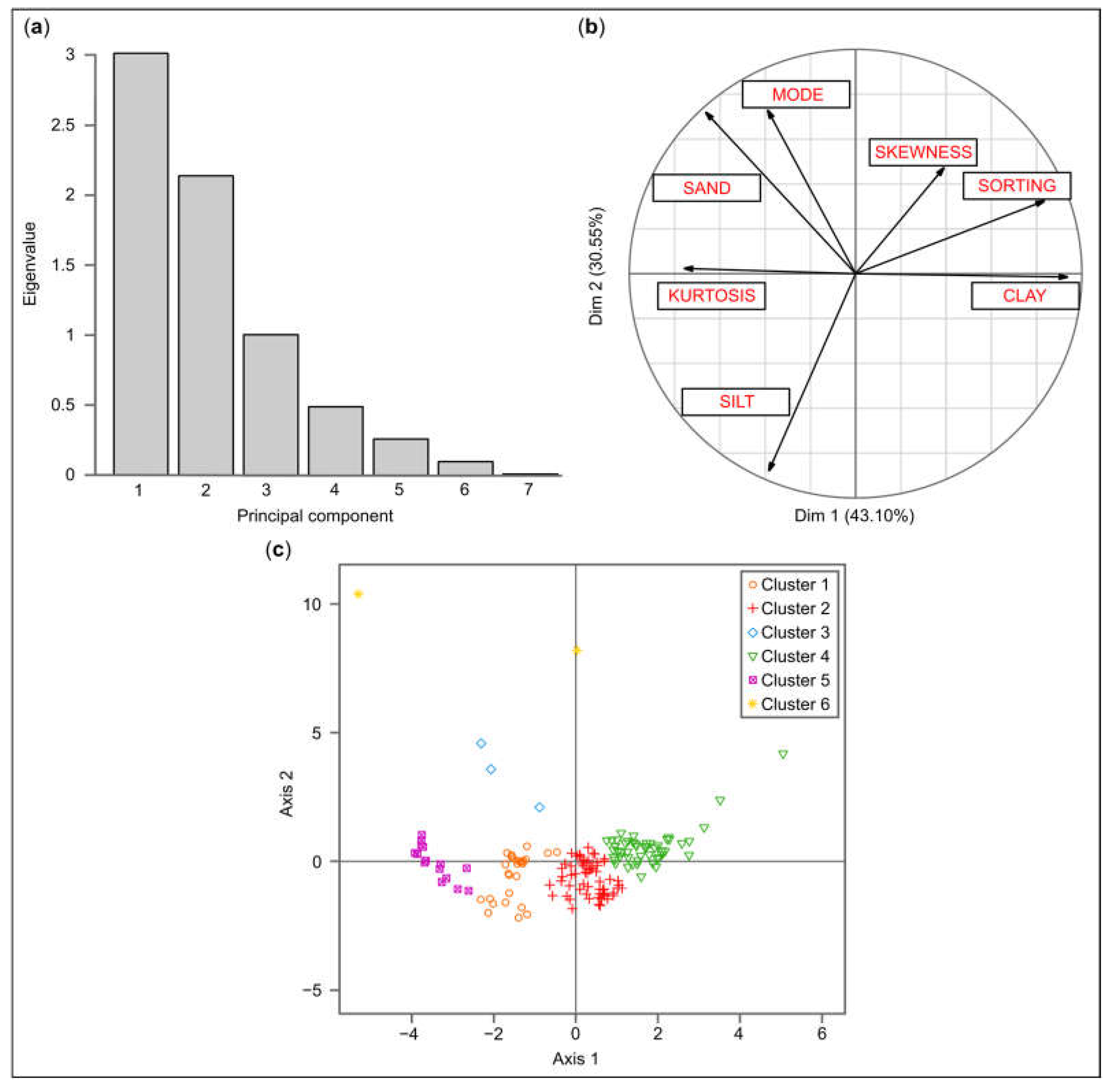
PCA-2 was conducted on a set of seven variables including four statistical variables (mode, sorting, skewness, kurtosis) and three textural variables (sand, silt, and clay fractions). The correlation matrix resulting from PCA-2 reveals several positive correlations: between sorting and clay fraction, mode and sand fraction, and kurtosis and sand fraction (

Table 5. Correlation matrix of seven statistical parameters.

	Mode	Sorting	Skewness	Kurtosis	Sand	Silt	Clay
Mode	1
Sorting	−0.03	1
Skewness	−0.18	0.34	1
Kurtosis	0.13	−0.6	−0.13	1
Sand	0.71	−0.31	0.15	0.47	1
Silt	−0.46	−0.54	−0.52	0.18	−0.36	1
Clay	−0.33	0.72	0.26	−0.59	−0.69	−0.43	1

). On the other hand, sand and silt fractions exhibit negative correlations with clay fraction and strong negative correlations with kurtosis and mode.

The results of the scree plot analysis indicate that PC1 explains 43.10% of the total variance while PC2 and PC3 contribute to 30.55% and 14.30% respectively (

Table 6. Total variance of the PCA-2.

Principal Component	Eigenvalue	% of Variance	% of Cumulative Variance
1	3.02	43.10	43.10
2	2.14	30.55	73.65
3	1	14.30	87.95
4	0.49	6.99	94.94
5	0.26	3.67	98.61
6	0.10	1.39	100

and Figure 9). Based on these results, only the scores of PC1 and PC2, which account for 74% of the overall variance, were included in the analysis. PC1 shows a positive correlation with clay content, sorting, and skewness. PC2 demonstrates a positive correlation with mode, sand fraction, and skewness, while it is negatively correlated with silt and clay fractions. The interpretation of PC1 suggests that it distinguishes between homogeneous and heterogeneous samples, while PC2 is structured by the grain size gradient.

5.3.4. HCA-2 Results

Using the scores from PC1 and PC2 of PCA-2, the HCA-2 analysis allows for the classification of samples into six distinct clusters (Figure 9). Cluster 1 (n = 29) consists of samples that exhibit bimodal to trimodal coarse silt characteristics. Cluster 2 (n = 60) group samples are categorized as silty to silty clay, often displaying skewness and platykurtic distribution. Cluster 3 is relatively small (n = 3) and comprises fine sand samples with some silt. The samples exhibit fine skewness to symmetry and platykurtic to mesokurtic distribution. Cluster 4 (n = 49) encompasses the finest samples, i.e., clay with fine silt. The samples exhibit fine skewness and are mainly platykurtic. Cluster 5 (n = 15) represents very coarse silt samples with sand content. The samples exhibit very fine skewness and a very leptokurtic distribution. At the least, Cluster 6 (n = 2) is associated with coarse sand and some silt. These samples show very fine skewness and a distribution ranging from platykurtic to mesokurtic.

Based on the memberships of the samples to the clusters resulting from HCA-2, the core CHA01 can be divided into four major units as shown in Figure 5. Unit U1 (900–869 cm) is characterized by its heterogeneity and comprises a mixture of samples from Clusters 2, 3, 4, and 6. Unit U2 (868–488 cm) can be subdivided into two highly homogeneous sub-units. U2a (869–755 cm) consists exclusively of Cluster 2 samples, while U2b (754–488 cm) includes only Cluster 4 samples. Unit U3 (487–189 cm) is dominated by samples from Clusters 2 and 5, and it is divided into three sub-units based on the proportions of samples from Clusters 1, 2, and 3. U3a (487–406 cm) is mainly associated with Cluster 5. U3b (405–290 cm) shows variations between Clusters 1 and 2, with the inclusion of two samples from Cluster 5. U3c (289–189 cm) exhibits fluctuations between Clusters 2, 3, and 4, but the overall trend is clearly dominated by Cluster 2. Unit U4 (188–0 cm) is primarily composed of samples from Clusters 1 and 2. U4a (188–142 cm) is dominated by Cluster 1 samples, while U4b (141–65 cm) consists exclusively of Cluster 2 samples. The top portion of U4, U4c (64–0 cm), solely comprises samples from Cluster 1.

5.3.5. PCA-3 Results

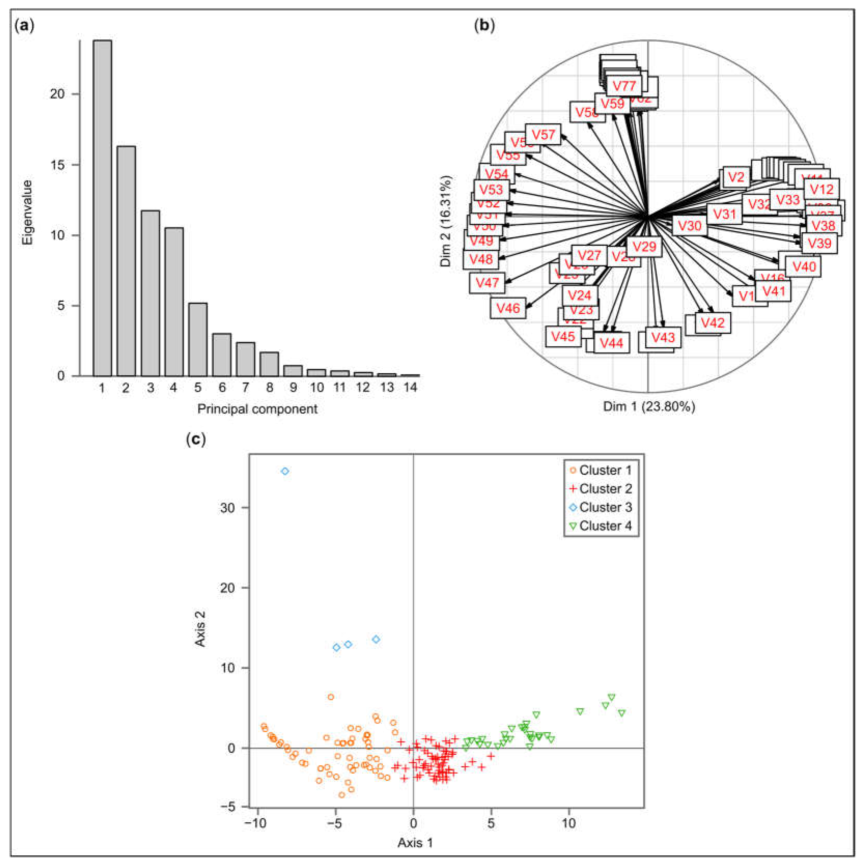
PCA-3 was conducted on 77 particle size classes that were present in the 158 samples. The first and second PCs account for 31% and 21% of the total variance, respectively (Figure 10). The first PC shows a positive correlation with fine-to-medium silt grain size classes, while it exhibits a negative correlation with coarse-silt-to-fine-sand grain size classes. The second PC distinguishes coarse grain size classes on the positive side from the finest grain size classes on the negative side. The interpretation of the first PC axis suggests a gradient from laminar to turbulent flow conditions, while the second PC axis represents the opposition between traction and suspension currents.

5.3.6. HCA-3 Results

HCA-3 used only PC1 and PC2 from PCA-3 since the third PC accounts for less than 12% of the variance. This analysis resulted in the identification of four sample clusters (Figure 10). Cluster 1 (n = 59) represents samples with medium grain size classes, ranging from coarse-to-medium silts. Cluster 2 (n = 65) consists of samples with medium-to-fine silts. Cluster 3 (n = 4) comprises multi-modal samples, which are the coarsest in the sequence, that range from fine-to-medium sands. Cluster 4 (n = 30) includes samples with fine silts and clay.

Based on these cluster assignments, the core CHA01 can be divided into four stratigraphic units (Figure 5). The lowest unit, U1 (900–869 cm), is primarily composed of samples from Clusters 1 and 2. U2 (868–488 cm) is further subdivided into three sub-units. U2a (868–744 cm) consists mainly of samples from Cluster 2. U2b (743–594 cm) shows variations between Cluster 2 and Cluster 4. U2c (593–488 cm) is the most homogeneous sub-unit, exclusively containing samples from Cluster 4. U3 (487–189 cm) exhibits a subdivision into three sub-units. U3a (487–394 cm) is highly homogeneous and comprises exclusively Cluster 1 samples. U3b (393–264 cm) alternates between Cluster 1 and Cluster 2 samples. U3c (263–189 cm) is characterized by great homogeneity and exclusively features samples from Cluster 2. Finally, U4 (189–0 cm) is primarily composed of Cluster 1 samples, with a small contribution from Cluster 2 samples.

5.4. CM Diagram

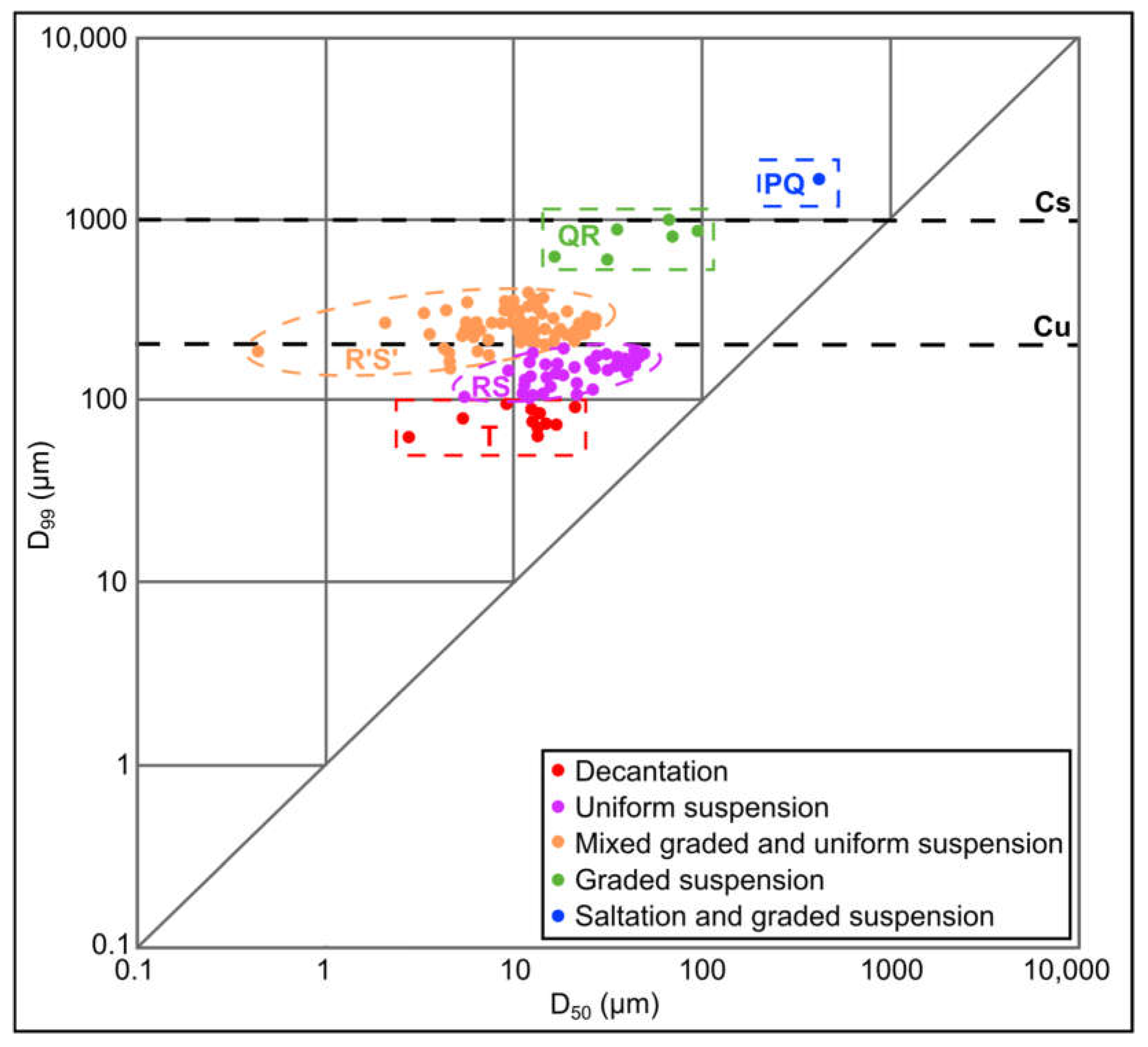
The CM diagram provides valuable insights into the characteristics of the fine alluvial plain deposits of the Charente River, specifically regarding transport and depositional processes (Figure 11). On the CM diagram, the PQ–QR segments represent graded suspension, the RS segment corresponds to uniform suspension, and the T segment indicates the decantation process for particles smaller than 100 μm. The RS segment can be further divided into two parts, following Arnaud-Fassetta [74]: the R’S’ segment represents a mixture of uniform suspension and graded suspension, while the RS segment solely indicates uniform suspension. Uniform suspension is limited to 200 μm (Cu), while graded suspension is confined to 1000 μm (Cs). Based on this analysis, three main types of sediment transport can be identified: (1) the minor graded suspension of fine and medium sands, (2) the predominant suspension of silty sand, sandy silt, and clayey silt, and (3) the minor decantation of silty clay deposits. According to the CM diagram, the CHA01 sequence can be subdivided into four units, each associated with a specific environment (Figure 5). U1 corresponds to a high-energy environment dominated by graded suspension. U2 represents a low-energy fluvial proximal plain linked to the R’S’ segment. U3 is characterized by the decantation process and uniform suspension. Finally, U4 is also associated with a low-energy fluvial proximal plain that is primarily characterized by the R’S’ segment.

5.5. End-Member Modeling Analysis

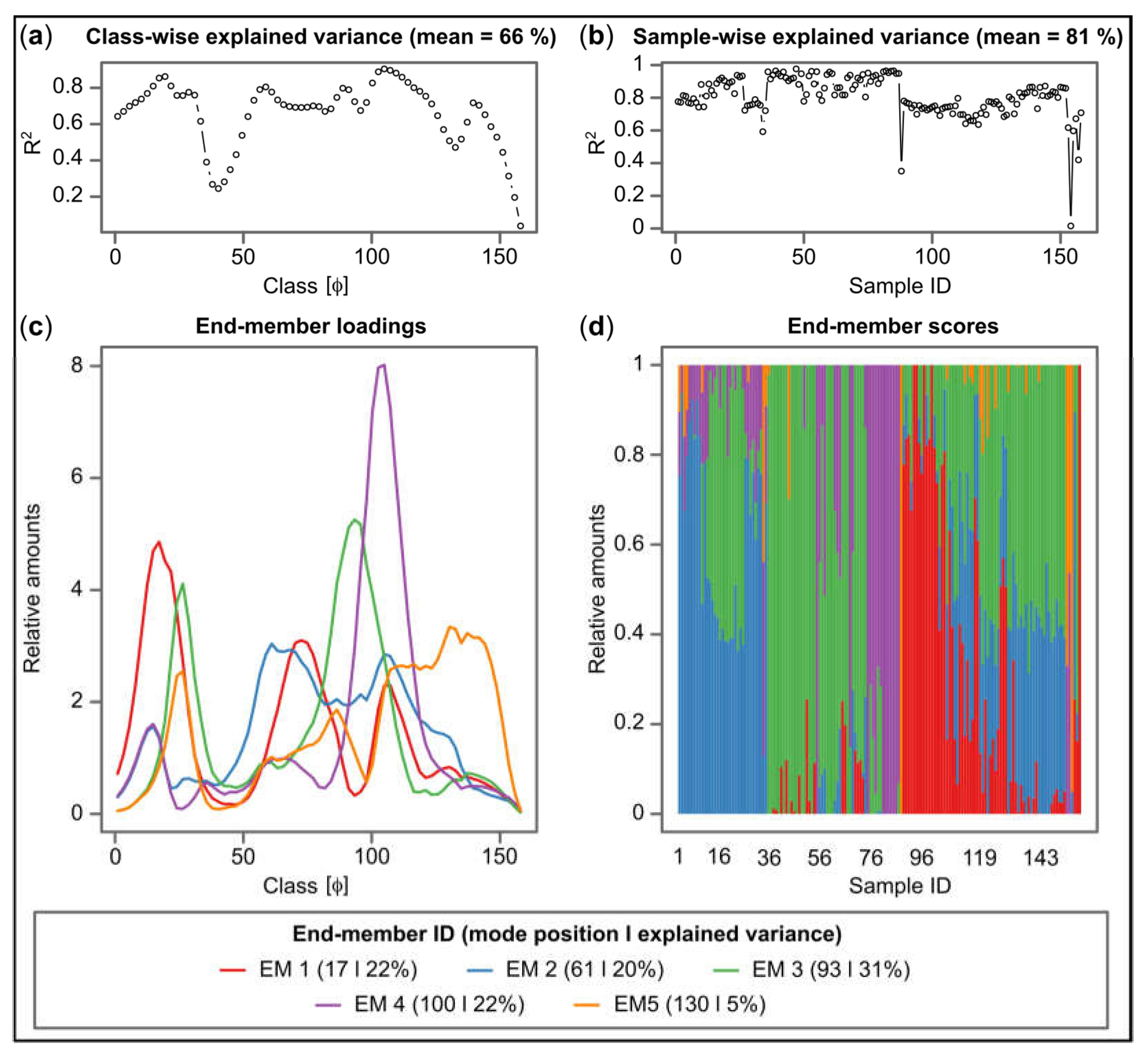
The final end-members model accounts for 66% of the variance among different classes and 81% of the variance among samples (Figure 12). It identifies five dominant end-members (EMs) with peak modes—at 17 μm (medium silt), 61 μm (very coarse silt), 93 μm (very fine sand), 100 μm (very fine sand), and 130 μm (fine sand). Each EM also includes minor modes. The explained variance for the five EMs is distributed as follows: EM1 (22%), EM2 (20%), EM3 (31%), EM4 (22%), and EM5 (5%). In the core CHA01, EM1 and EM2 dominate, accounting for 42% of the total variance. These end-members represent medium-to-very-coarse silts. EM3 to EM5 contribute to the remaining 58% of the total variance and correspond to very-fine-to-fine sands (Figure 12). Further division of the core reveals four major units (Figure 5).

U1 (900–869 cm) exhibits a patchy distribution of EM abundances. However, EM1 and EM3 dominate the upper part of the unit, while EM4 and EM5 (the coarser end-members) have higher contributions in the lower part.

U2 (868–488 cm) mainly consists of a combination of EM1, EM2, and EM3. The proportion of EM1 increases from the base to the top, while the contributions of EM2 and EM3 decrease. EM5 has a minor contribution, but it indicates the discrete recording of high-energy events (i.e., fine sand layers). Based on the relative proportions of EM1, EM2, and EM3, U2 can be further divided into three sub-units. U2a (868–744 cm) shows a significant contribution from EM2 and EM3, while the contribution from EM1 is negligible (less than 10%). In U2b (743–594 cm), the contributions of EM2 and EM3 remain dominant, but there is a slightly higher contribution of EM1, ranging from 50% to 60%. In U2c (593–488 cm), the contribution of EM1 remains high (more than 70%), while the contributions of EM2 and EM3 decrease compared to those of the two previous sub-units.

U3 (487–189 cm) predominantly consists of a mixture of EM3 and EM4 (Figure 5). The abundance of EM4 decreases from the bottom to the top of the unit, while the contribution of EM3 increases. EM1, EM2, and EM5 remain minor components. Based on these observations, U3 can be divided into three sub-units. The upper sub-unit (487–406 cm) is dominated by EM4. The middle sub-unit (405–290 cm) exhibits a high contribution of EM3, while the contribution of EM2 is lower compared to U3a. The lower part (289–189 cm) is predominantly composed of EM3. Both U3b and U3c show prominent peaks of EM1, which account for 15–25% of the composition but are distributed unevenly within the two sub-units.

U4 (188–0 cm) is composed of a mixture of EM2, EM3, and EM4. The contribution of EM5 is negligible. U4 can be subdivided into three sub-units (Figure 5). U4a (188–142 cm) exhibits a high contribution of EM2 and a low contribution of EM3 and EM4. In U4b (141–50 cm), EM3 dominates with a contribution of approximately 50–60%, while EM2 contributes between 40% and 50%. The abundance of EM4 is very low—less than 10%. Finally, the top sub-unit (U4c, 49–0 cm) shows a significantly high contribution of EM2. EM4 and EM5 are minor components, accounting for less than 20%, while EM3 is absent.

6. Discussion

The application of five different particle size processing methods to core CHA01 reveals a general agreement in the overall results from a macroscopic perspective. However, when using methods based on first-order statistical moments such as the mean and median, which are the most employed, the results are poorly conclusive. The high homogeneity of the values makes it challenging to discern distinct stratigraphic units within the studied sequence. Analyzing the modes (first, second, and third order) reveals that focusing solely on the two most abundant ones is of limited value. The presence of abundant fine sediments masks minor variations in grain size. This homogeneity is attributed to the low contrast in sediment sources within the watershed. The use of the tertiary mode, which exhibits stronger variations, could be more promising. Previous research by Duquesne [35] has also demonstrated that relying on the D₉₀ indicator provides limited information. Ultimately, the application of these indicators allows, at best, a broad subdivision into macro-scale (i.e., metric to sub-metric) units, i.e., third-order stratigraphic units [75].

Texture analysis, another commonly used method for describing grain size variations in sedimentary sequences, is highly dependent on the classification scheme and yields contrasting results. This is partly due to both the number of categories used by each method (ranging from 5 to 11) as well as the distribution and fineness of the silt and clay sub-categories. However, regardless of the chosen method, the sand–silt–clay classification scheme helps refine the results obtained from simple statistical methods and facilitates a more detailed subdivision into sub-units or second-order units. It is noteworthy that there is a strong agreement among the different classification methods regarding the main boundaries (first-order divisions). The UK SSEW and Aisne methods demonstrate a high level of convergence and appear to be well-suited for classifying fine sedimentary sequences, such as those found in the low-energy alluvial plains of rivers.

The application of multivariate modeling methods combining PCA and HCA provides contrasting results and is highly sensitive to the choice of input data. When PCA is applied, considering only the first-order statistical moments and sorting index (PCA-1 and HCA-1 case), the results are the least convincing. It appears that a significant portion of the relevant information is “lost” when using these indices. However, in rare cases, it can provide valuable information, particularly for analyzing spatial data [21] but is less conclusive for stratigraphic approaches. Including grain size classes (sand–silt–clay content) in the dataset, as in PCA-2, allows for more refined results but still proves inconclusive. Once again, the use of aggregated data results in a partial loss of information. Ultimately, it is PCA-3 performed on raw grain size data that produces the most interesting and informative outcomes.

Although Ward’s method was exclusively used in this study to identify groups of similar sediment samples, alternative partitional clustering methods such as k-means or k-medoids could also be considered, particularly when working with categorical data. The silhouette coefficient can be employed to determine the optimal number of clusters in these methods. In both cases, the objective is to minimize the error between the empirical mean of a cluster and the points within the cluster. Unlike k-means clustering, which uses the mean as the cluster center, k-medoids clustering involves selecting an actual point from the data set as the center. The k-medoids method may be preferred as it is more robust and less sensitive to outliers.

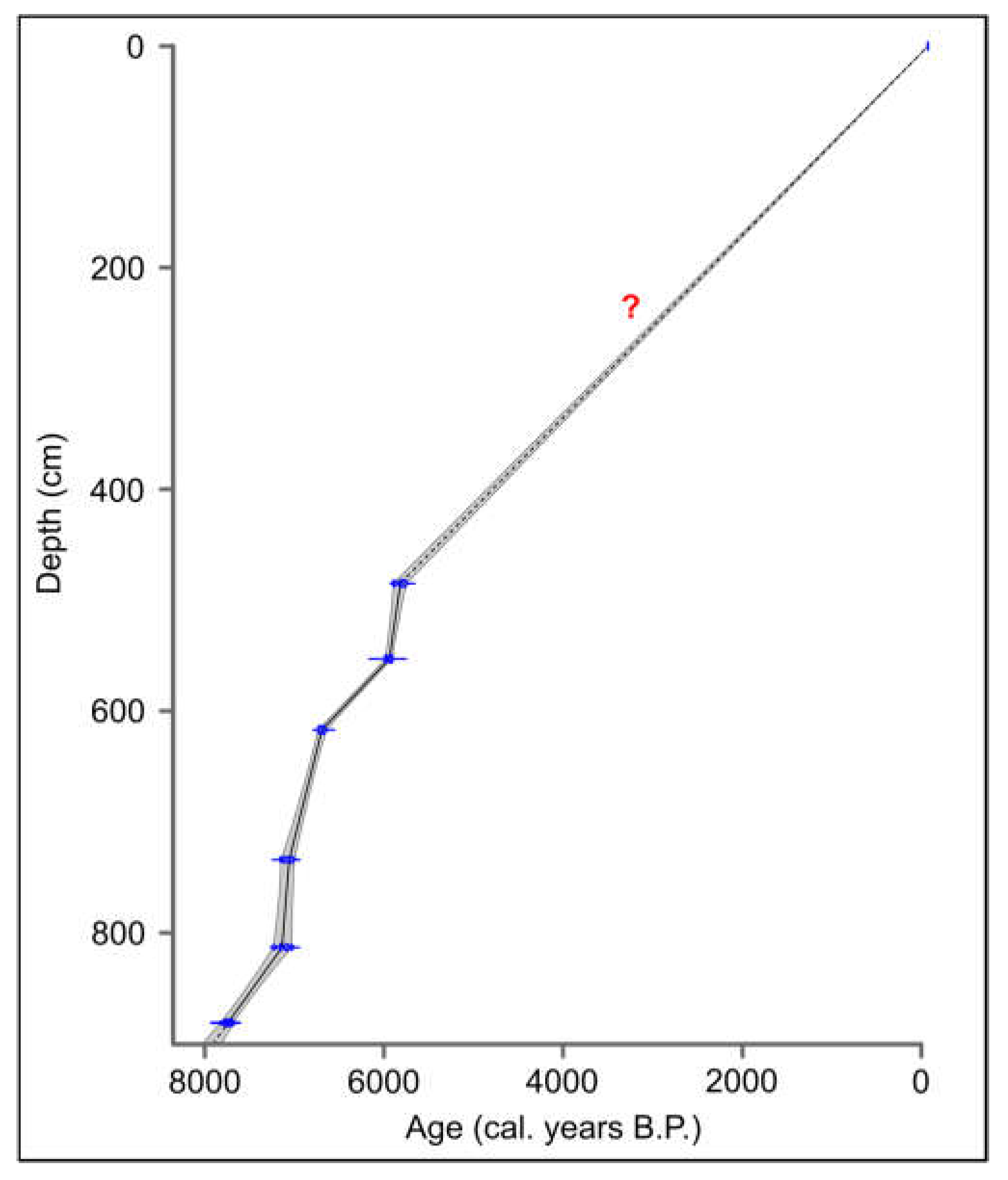
Based on these different methods, the CHA01 sequence can be divided into four units, each associated with a specific sedimentation environment. The lower unit, U1, is characterized by coarser and more heterolithic sediments, indicating deposition in a high-energy channel environment. This unit is believed to have been formed during the 8.2 Rapid Climate Change event [76] based on the age–depth model. U1 is atypical and likely represents deposits from a braided unconfined channel system. The sediment sources for this unit include coarse-to-medium gravels and sands derived from inherited periglacial formations that were still active at the time of its formation. U2 represents a typical low-energy fluvial proximal floodplain located near the base level. This unit shows an increase in tidal influence, which is consistent with local data on the Holocene sea-level rise [77,78]. The rapid rise in sea level between 8 and 6 ka B.P. led to high rates of aggradation and the formation of floodplains and swamps. U3 is characterized by an increase in mean grain size, particularly in the finer fractions (EM1). It is interpreted as a natural levee [79,80,81] and indicates a shift from sedimentation dominated by tidal processes to sedimentation dominated by fluvial processes and overflows. Lastly, U4 exhibits an end-member structure like U2 and is also interpreted as a low-energy fluvial plain.

7. Conclusions

This paper provides a comprehensive review of commonly used methods for processing grain size data ranging from elementary statistical approaches to more advanced techniques such as multivariate statistics and the innovative EMMAgeo method. The findings suggest that traditional statistical methods including statistic moments, sorting indices, and textural analysis have limited usefulness in interpreting low-contrasted alluvial records. While means of textural classification, such as ternary diagrams, can provide more informative results, the selection of an appropriate classification scheme is crucial and is often lacking in discussion.

The application of multivariate statistics, specifically PCA pre-processing and HCA classification, shows that their effectiveness strongly depends on the choice of input variables. Contrary to common practice, using raw data appears to be more favorable than relying on elaborated statistical indices. However, it is important to note that multivariate analysis should be applied solely to non-zero values to avoid statistical bias, which can be a limitation in cases where there are contrasting grain size records.

The EMMAgeo method shows promise as an innovative approach. However, it is necessary to establish clearer connections between the obtained end-member classes and sedimentological processes. Further research and refinement are needed to enhance the interpretation of EMMAgeo results in relation to sedimentological processes.