Resource Profiling and Performance Modeling for Distributed Scientific Computing Environments

Abstract

Scientific applications often require substantial amount of computing resources for running challenging jobs potentially consisting of many tasks from hundreds of thousands to even millions. As a result, many institutions collaborate to solve large-scale problems by creating virtual organizations (VOs), and integrate hundreds of thousands of geographically distributed heterogeneous computing resources. Over the past decade, VOs have been proven to be a powerful research testbed for accessing massive amount of computing resources shared by several organizations at almost no cost. However, VOs often suffer from providing exact dynamic resource information due to their scale and autonomous resource management policies. Furthermore, shared resources are inconsistent, making it difficult to accurately forecast resource capacity. An effective VO’s resource profiling and modeling system can address these problems by forecasting resource characteristics and availability. This paper presents effective resource profiling and performance prediction models including Adaptive Filter-based Online Linear Regression (AFOLR) and Adaptive Filter-based Moving Average (AFMV) based on the linear difference equation combining past predicted values and recent profiled information, which aim to support large-scale applications in distributed scientific computing environments. We performed quantitative analysis and conducted microbenchmark experiments on a real multinational shared computing platform. Our evaluation results demonstrate that the proposed prediction schemes outperform well-known common approaches in terms of accuracy, and actually can help users in a shared resource environment to run their large-scale applications by effectively forecasting various computing resource capacity and performance.

1. Introduction

Distributed scientific computing platforms such as research Grid, volunteer computing platform and Cloud [1,2] make it possible to share and integrate hundreds of thousands of heterogeneous computing resources from multiple domains organized into Virtual Organization (VO) [3]. VO enables users to access a large amount of computing resources as a single virtualized platform, and offers unique opportunities to the research community for modeling and simulating complex scientific and engineering problems such as discovering new drug, diagnosing medical conditions, forecasting weathers, managing stock portfolios, simulating earthquake data, etc. Furthermore, recent emerging applications from many scientific domains such as astronomy, physics, pharmaceuticals, and chemistry, which typically involve millions of loosely-coupled tasks with relatively short per task execution times have expedited the expansion of traditional High-Throughput Computing (HTC) into Many-Task Computing (MTC) [4,5]. These applications are computationally intensive and can benefit from the integrated computing capability of VOs in the PetaFLOPS range at a reasonable cost [6].

However, the shared resources inside the virtual organization are inherently unreliable, volatile, and not always accessible. Additionally, computing resources are geographically distributed across numerous sites and are managed by separate independent resource providers with varying objectives, priorities, and management policies within a VO [7]. As a consequence, the application running time or completion time (makspan) of a job can be typically hours or even for days, which makes a substantial impact on the reliability of distributed systems, since reliability is often measured in terms of the probability that a job will be successfully completed by the system [1]. Therefore, accurate assessment of distributed resource capacity and performance will certainly increase the efficiency of job scheduling and the overall user satisfaction. With the help of precise resource information and consistent performance of the shared computing environment, it can provide processing power that exceeds the capability of even the most powerful parallel computer system (i.e., Supercomputers) by effectively integrating exceedingly diverse physical resources into a single virtual resource [8].

Since large-scale distributed computing resources are often unstable and heterogeneous, today’s key research question is how to create a model-based scheduler [9] that guarantees predictable resource capacity and performance on an unpredictable distributed platform. To address this problem, we have developed SCOUT system [10,11] which can periodically profile and manage information about each computing elements (CE) of the VO. This profiled data inspired us to develop a new resource prediction model that can enable users to effectively execute their tasks across VO member sites with higher probabilities of allocating available CPU cores and completing tasks in the shortest time possible.

In this paper, we present novel resource profiling and performance prediction models by using linear combination of past predicted values and recent profiled data from our SCOUT system in order to support large-scale applications in distributed scientific computing environments. Specifically, our predication models include Adaptive Filter-based Online Linear Regression (AFOLR) and Adaptive Filter-based Moving Average (AFMV). In order to evaluate the effectiveness of proposed models, we also conducted microbenchmark experiments on the Biomed VO [12] which is a large-scale international and interdisciplinary virtual organization providing tens of thousands of CPU cores to scientific communities. Our evaluation results demonstrate that the proposed prediction schemes outperform well-known common approaches in terms of accuracy, and actually can help users in a shared resource environment to run their large-scale HTC/MTC applications by effectively forecasting various computing resource capacity and performance. To summarize, the contributions of our paper can be as follows:

• Design of novel resource profiling and prediction models including Adaptive Filter-based Online Linear Regression (AFOLR) and Adaptive Filter-based Moving Average (AFMV) by effectively employing linear combination of past predicted values and recent profiled data
• Implementation of our proposed schemes on top of SCOUT system which can periodically profile and manage information of distributed scientific computing environments
• Application of the proposed scheme and policies to a real large-scale international and interdisciplinary computing environment for running many-tasks
• Comprehensive evaluation results of AFOLR and AFMV models including quantitative analysis and microbenchmark experiments for Many-Task Computing (MTC) workloads

The rest of this paper is structured as follows. In Section 2, we briefly describe motivation & background of this study, and present some of related research work. Section 3 presents our resource profiling and forecasting system along with various prediction methodologies including proposed adaptive profiling models. Section 4 presents comprehensive evaluation results of our proposed schemes and Section 5 summarizes and throws light on areas for further investigation. Finally, Section 6 highlights our conclusions and future work directions.

2. Background and Related Research Work

This section begins with discussions of motivation and background study for our research (Section 2.1), followed by the presentation of related research work (Section 2.2) aimed at modeling the performance of distributed computing resources in terms of availability, resource characteristics, application run time, CPU & memory capacity, etc.

2.1. Background Study

The large-scale scientific computing platform pools resources from many administrative domains, individuals, and institutions to create a Virtual Organization (VO)  [3]. VO enables users to access the large amount of computing resources as a single virtualized computing platform distributed across multiple resource provider locations. The interactions between users, VOs, and shared resources are shown in Figure 1. A user may be a member of one or more VOs, and the same resources can be shared across multiple VOs. Additionally, Figure 1 demonstrates that a VO is composed of a number of Computing Elements (CEs). A CE is a collection of computing resources that are physically located at a resource provider site (i.e., a cluster, supercomputer, a computing farm), and the cluster is a collection of Worker Nodes (WNs) that actually perform the tasks.

Figure 1. Large-scale distributed computing infrastructure and interactions between users, VOs, and resource providers.

Shared resources are inherently very dynamic and volatile which implies that a resource that was accessible at a certain time or day in the past may not be available in the future for an extended length of time or for a few days at a later time. It is also difficult to locate the available free computing resources since shared resources are constantly departing and rejoining the VO for a variety of reasons including load balancing, hardware/software maintenance, etc. Moreover, the capacity of each computing element, which is defined as the number of available CPU cores, varies significantly across the participating institutions and also fluctuates over time. Furthermore, the performance (i.e., response time) of each resource varies greatly, potentially due to the end-to-end network bandwidth, current system load, local scheduling strategy, and so on.

For example, Figure 2a presents a typical one-day available CEs and the amount of accessible free CPU cores at the BIOMED VO [12], whereas Figure 2b depicts the average response times of each CE. As we can see from the Figure 2, not only the number of CPU cores available in each CE is varied, but also the response times are, which makes it difficult to forecast the available resources and associated performance of each CE in a Virtual Organization. On the other hand, there is currently no effective Information Service (IS) that can deliver accurate information about shared resources and their states. This information is critical for identifying and monitoring VO resources as well as scheduling user tasks on the relevant CEs.

Figure 2. Resource Capacity and Response Time of Each CE on BIOMED VO.

In order to address these obstacles and challenges, we have been interested in understanding the computing resource behaviors of VOs over time periods ranging from a few days to weeks that can be utilized for developing an adaptive resource profiling model that takes into account both the resource availability and associated performance. Our ultimate goal is to evaluate the behaviors of CEs and utilize this dynamic information to predict the probability that a CE will be able to supply a certain number of free CPU cores with reasonable amount of response time.

2.2. Related Work

Loosely-coupled virtual organizations (VOs) provide significant scalability and cost advantages over conventional distributed systems. However, the availability of nodes and the performance capacity (i.e., number of CPU cores, response time, queuing delay, etc.) of their resources vary significantly in these systems. The performance prediction aids both the Resource Management System (RMS) and users in making resource consumption decisions that are optimal for Quality of Service (QoS) compliance. As a consequence, substantial research on performance modeling of large-scale distributed computing systems, such as Grid [13,14], Peer-to-Peer [15], and Cloud [16], have been conducted.

Figure 3 depicts the most commonly used approaches for performance modeling, which consists of application-oriented and resource-oriented predictions. Application-oriented performance models project the execution times of submitted jobs on the distributed system or profile the application based on its runtime (i.e., short or long running times) or resource utilization patterns such as CPU or I/O intensive, or both [17]. The application-oriented method has the benefit of directly addressing the scheduler’s ultimate performance measures (deadlines, runtimes, etc.) [18].

Figure 3. Types of performance modeling for large-scale distributed system.

In contrast, resource-oriented performance models are often used to forecast host availability, resource reliability, CPU capability, and end-to-end network bandwidth. A prospective job’s background load may be calculated using a resource-oriented strategy. This is directly related to predicting the available CPU capacity or resource level [18]. In this method, predicting the resource level is achievable regardless of the number of job tasks running at any given moment.

To make accurate predictions, researchers have typically used time series algorithms to learn from past information or trace data. To model resource performance, several types of resources are explored including CPU load, CPU availability, memory, queuing delay, network bandwidth, disk speed, and so on [19].

Dinda et al. [20] examined the performance of numerous linear time series models for predicting the average load on a host system, including Autoregressive (AR), Moving Average (MV), Autoregressive Moving Average (ARMV), and Autoregressive Integrated Moving Average (ARIMV). According to their results, the Autoregressive technique is best suited for estimating CPU load on a single host. However, these kinds of static prediction techniques are effective only for the workloads that are relatively steady.

Javadi et al. [21] have found a subset of hosts that have common statistical characteristics regarding availability. Additionally, they organize hosts by functionality, which helps with scheduling and hence minimizes the makspan. Historical data from SETI@Home was used to simulate resource availability [22]. The authors of [23] investigated the characteristics of node availability in a large-scale shared computing system. They investigated PlanetLab’s [24] eligibility period for computing resources, built heuristic models, and projected idle resource capacity using PlanetLab utilization data traces. These preceding performance models often interpret resource availability as a binary state, implying that resources are either accessible or unavailable. However, the authors provide a multi-state availability model in the study [25] to capture the genuine states of resources such as available, user present, CPU threshold exceeded, job eviction, and unavailable.

The Network Weather Service (NWS) [26] is a well-studied system for monitoring and predicting distributed resources by using statistical techniques such as running average, sliding window average, and the last measurement. To decrease prediction errors and choose the best predictors, NWS employs a number of adaptive techniques including adaptive window average, adaptive window media, media filter, a-trimmed mean, stochastic gradient, and autoregressive algorithms. It properly forecasts CPU availability and network bandwidth (TCP end-to-end throughput and TCP end-to-end delay).

Table 1 summarizes significant research work on resource performance modeling for distributed environments published in the last two decades. Most of these studies use traditional time series prediction techniques. The historical data traces of a resource may be stored and used to forecast future trends, however, it is difficult to efficiently utilize them by using one of the prediction methodologies. In reality, none of the mentioned prediction methods have been proved to be 100% accurate. Furthermore, it is clear that certain methods are more effective than others in achieving a specific goal. As a consequence, at this moment, it is crucial to consider combining different ways to get the best results.

Table 1. Summary of related work on resource performance modeling for distributed systems.

Resource Type	Related Study
CPU load	Dinda et al. [20], Smith et al. [17], Verma et al. [27]
Host Machine/Node	NWS [26], Javadi et al. [21], Padhye et al. [23], SCOUT [10]
Network Bandwidth	NWS [26], EDG ROS [28], Faerman et al. [29]
Memory	FACE [30], FAST [31]

Recently, an increasing number of attempts has been undertaken to predict the resource characteristics of distributed systems by using neural networks [32] and deep learning techniques [33,34]. However, these techniques are very complex, resource intensive, and time demanding. Furthermore, emerging applications [35] such as Unmanned Aerial Vehicles (UAV), robotics, and self-driving cars need lightweight and simple adaptive resource profiling methods.

In this study, we provide profiling models based on the linear difference equation [36] which can effectively predict anticipated values by combining the past data with current profiled information about computing resources. As a result, the models are computationally efficient, interpretable, and self-adaptive which can be applied to a real large-scale international and interdisciplinary computing environment for running many-tasks.

3. Resource Profiling and Performance Modeling

In this section, we present details of our Adaptive Filter-based Online Linear Regression (AFOLR) and Adaptive Filter-based Moving Average (AFMV) resource profiling and prediction models (in Section 3.2.3 and Section 3.2.4 respectively). Both AFOLR and AFMV models can capture the time-varying characteristics of underlying computing resources which means that they will have less prediction errors even for highly dynamic resources (as we will quantitatively see from Section 4.1). As comparison models, we also adopted Online Linear Regression and Moving Average (described in Section 3.2.1 and Section 3.2.2) which are well-known and conventional prediction models.

First of all, we briefly introduce the overall process of resource profiling and forecasting which can be effectively utilized for a large-scale job scheduling system.

3.1. Resource Profiling and Forecasting Process

The overall resource profiling and forecasting procedure is illustrated in Figure 4. Our SCOUT system [10,11] (denoted as “Resource Monitor & Profiler” in the Figure 4) periodically profiles and records information about each computing element (CE) of the VO including the number of CPU cores, queue waiting time, and average task response time. This information can be effectively utilized to forecast resource capability and performance such as CPU core availability and expected user response time.

Figure 4. The overall process of identifying and forecasting resource capacity.

Our HTCaaS (High-Throughput Computing as a Service) [37,38] system could take advantage of this forecasting data in order to efficiently submit a vast number of tasks by using all available computing resources in the Grid, Supercomputers, and Cloud. For example, the drug repositioning simulation needed about 80,000 docking tasks and we were able to successfully complete the experiment by leveraging 2300 CPU cores foretasted by our models. Basically, HTCaaS aims to provide researchers with ease of exploring large-scale and complex HTC problems by leveraging Supercomputers, Grids, and Cloud by effectively hiding heterogeneity and complexity of harnessing different types of computing infrastructures from users. HTCaaS has been effectively integrated with national Supercomputers in Korea, international computational Grids, and Amazon EC2 resulting in combining a vast amount of computing resources to support most challenging scientific problems.

3.2. Resource Profiling and Prediction Models

Our proposed profiling models are based on the linear difference equation which combines historical projected values with current profiled information in a VO to make the model computationally efficient, interpretable, and scalable. To measure the past predictions, we employ Online Linear Regression (OLR) and Moving Average (MV) in the proposed models. In this section, we first present the basics of OLR and MV, and then describe our proposed models in further detail.

3.2.1. Online Linear Regression (OLR)

Typically, the measured or real outputs are highly variable because resource instances in a distributed scientific computing system are stochastic in nature. The conventional prediction methods such as linear regression (LR), autoregressive (AR) predict future resource availability using historical n data points. Recent dynamic changes in resource availability can be easily captured if we rely on the most recent trends of data rather than all historical n points information.

A simple linear model of one explanatory variable has two parameters such as ${\beta }_0$ and ${\beta }_1$ expressed as in the following Equation (1). Parameters ${\beta }_0$ and ${\beta }_1$ are estimated from the n observed data set. In the Equation (1), the subscript i denotes the observational unit, where $\mathit{i}=\left\{1,2,\dots ,n\right\}$ and n is the total number of observed data.

$$Y_i={\beta }_0+{\beta }_1{X}_i$$

(1)

The least squares estimation method [39] has been widely applied to estimate the parameter values because this technique provides the smallest possible sum of squared error of the observed Y${}_i$ from the estimates $\widehat{Y}$. Let ${\widehat{\beta }}_0$ and ${\widehat{\beta }}_1$ be numerical estimated values of the parameters ${\beta }_0$ and ${\beta }_1$ respectively. The Equation (1) can be written as follows:

$${\widehat{Y}}_i={\widehat{\beta }}_0+{\widehat{\beta }}_1{X}_i$$

(2)

The least squares principle chooses ${\widehat{\beta }}_0$ and ${\widehat{\beta }}_1$ in a way that minimizes the sum of squared ($SS$) of magnitude of the residual $ϵ$. The $i\mathrm{th}$ residual ${ϵ}_i$ is the difference between the real output Y and the estimated output $\widehat{Y}$ at the data point i.

$$\begin{array}{cc}\hfill SS\left(Residual\right)& =\sum _{i=1}^n{(Y_i-{\widehat{Y}}_i)}^2=\sum _{i=1}^n{ϵ}_i^2\hfill \\ \hfill & =\sum _{i=1}^n{(Y_i-{\widehat{\beta }}_0-{\widehat{\beta }}_1{X}_i)}^2\hfill \end{array}$$

(3)

Applying the derivatives with respect ${\beta }_0$ and ${\beta }_1$, we can solve the Equation (3) to estimate the parameters.

$$\frac{\partial SS}{\partial {\beta }_0}=-2\sum _{i=1}^n)(Y_i-{\widehat{\beta }}_0-{\widehat{\beta }}_1{X}_i)=0$$

(4)

$$\frac{\partial SS}{\partial {\beta }_1}=-2\sum _{i=1}^n)(Y_i-{\widehat{\beta }}_0-{\widehat{\beta }}_1{X}_i)=0$$

(5)

Simplifying the Equations (4) and (5) yields the ${\widehat{\beta }}_0$ and ${\widehat{\beta }}_1$ as follows:

$${\widehat{\beta }}_0=\overline{Y}-{\widehat{\beta }}_1\overline{X}$$

(6)

$${\widehat{\beta }}_1=\frac{{\sum }_{i=1}^n(X_i-\overline{X})(Y_i-\overline{Y})}{{\sum }_{i=1}^n{(X_i-\overline{X})}^2}$$

(7)

where $\overline{X}$ and $\overline{Y}$ are the means of the $X_i$ and $Y_i$ respectively. It can be noted from the Equation (7) that $\left(X_i-\overline{X}\right)$ and $\left(Y_i-\overline{Y}\right)$ denote observations expressed as deviations from their sample mean $\overline{X}$ and $\overline{Y}$ respectively. Therefore, estimation of parameters give the linear regression model equation as follows:

$${\widehat{Y}}_i={\widehat{\beta }}_0+{\widehat{\beta }}_1{X}_i$$

(8)

Online regression modeling makes forecasting by using a window with size w which contains the latest profiling information, i.e., w data points out of n (where $w<n$). Thus, predicting based on dynamic w interval is known as Online Linear Regression (OLR) model and the coefficient parameters ${\beta }_0$ and ${\beta }_1$ are estimated based on the Equations (9) and (10) where ${\overline{X}}_w$ and ${\overline{Y}}_w$ are the mean of sample data over w interval. This model is also known as moving linear regression because w is moving towards the recent trends.

$${\widehat{\beta }}_0^w={\overline{Y}}_w-{\widehat{\beta }}_1^w{\overline{X}}_{w}wherei=(1,2,\dots ,n-w+1)$$

(9)

$${\widehat{\beta }}_1^w=\frac{{\sum }_{j=i}^{w+i-1}(X_j-{\overline{X}}_w)(Y_j-{\overline{Y}}_w)}{{\sum }_{j=i}^{w+i-1}{(X_j-{\overline{X}}_w)}^2}$$

(10)

For example, suppose we have 100 days (here n = 100) of SCOUT profiling information including the number of available CPU cores in each computing element. The Online Linear Regression (OLR) method calculates the regression coefficient parameter ${\beta }_0$ and ${\beta }_1$ using the most recent w days of profiled data. The length w can be 1 week, 10 days or so on depending on user preference for prediction. Therefore, the online linear regression model equation can be calculated as follows:

$${\widehat{Y}}_{w+i}={\widehat{\beta }}_0^w+{\widehat{\beta }}_1^w{X}_{w+i}$$

(11)

Algorithm 1 describes the OLR approach in depth. Here, L is the collection of all computing elements in a VO, n denotes the number of datapoints stored in the database, w denotes the user’s preferred window size (the size of the window can be adjusted), i refers $n-w+1$, and D denotes all profiling data gathered by the SCOUT system.

Algorithm 1: Online Linear Regression (OLR).

3.2.2. Moving Average (MV)

Moving average (MV) is widely used especially when data is highly variable. Profiling information close to the recent n points are typically more relevant than data further away from the latest because computing resources in a distributed scientific computing system dynamically changes over some periods of time possibly due to addition of new resources, removal of old resources or even failures.

Moving average follows the recent trend of the data, not an actual average of the data and it is useful for smoothing out the noisy raw data. Suppose the sequence of data $X=\left(x_1,x_2,\dots ,x_n\right)$, a w-moving average (w interval) is defined from $X_i$ by taking the arithmetic mean of sub sequences of w terms (as we can see from Equation (12)).

$$M{V}_{w+i}=\frac{1}{w}\sum _{j=i}^{w+i-1}{X}_{j}wherei=(1,2,\dots ,n-w+1)$$

(12)

For instance, if our window size is 3, then on day 4, the moving average is generated by taking the simple average of the preceding three days’ available CPU cores for that specific CE, and the procedure is repeated. If we have six days of data (201, 202, 230, 213, 180, and 190), then the $MV$ on day 4 will be 211, on day 5 will be 215 and so on.

3.2.3. Adaptive Filter-Based Online Linear Regression (AFOLR)

A difference equation relates the current and past predicted values to current and past input values [36]. Most commonly expressed difference equation is as follows:

$$Y\left(k\right)=Y(k-1)+u\left(k\right)$$

(13)

Here, $Y\left(k\right)$ means the last estimated output value which is calculated using past $Y(k-1)$ estimated values and the latest actual input value $u\left(k\right)$. Filter technique is widely applied in the field of prediction modeling because it helps to eliminate the noise from the output and smooth the estimated value if the system is extremely dynamic (e.g., available free CPU cores, average response time in a distributed scientific computing environment). Applying simple filter technique to the prediction model of the Equation (13) is as following:

$$Y\left(k\right)=(1-\alpha )\ast Y(k-1)+\alpha \ast u\left(k\right)$$

(14)

For $\alpha$ value close to 1 means more heavily relying on the current measurement $u\left(k\right)$, and if the value of $\alpha$ becomes close to 0, we make decisions more based on previous estimation $Y(k-1)$ (i.e., 0 $⩽\alpha ⩽1$).

Our proposed AFOLR prediction model forecasts depending on the last predicted values $Y(k-1)$ as well as recent profiled information. AFOLR model employs the Online Linear Regression model (discussed in Section 3.2.1) to estimate the last predicted value $Y(k-1)$ within the most recent w intervals, together with the latest profiled data $u_{scout}\left(k\right)$. Therefore, our proposed AFOLR model can be represented using the following equation:

$$Y\left(k\right)=(1-\alpha )\ast Y_{OLR}^w(k-1)+\alpha \ast u_{scout}\left(k\right)$$

(15)

The proposed AFOLR model basically integrates online linear regression (OLR) to make it computationally efficient, interpretable, and scalable as illustrated in the Algorithm 2. It uses the OLR determined in the w-window size as well as the latest profiled information $u_{scout}$.

Algorithm 2: Adaptive Filter-based Online Linear Regression (AFOLR).

3.2.4. Adaptive Filter-Based Moving Average (AFMV)

In order to address more steep fluctuation of resource availability and reflect the recent trend, we have devised Adaptive Filter-based Moving Average (AFMV) model by employing the moving average technique (as discussed in Section 3.2.2). AFMV prediction model applies similar rationale as AFOLR model so that it estimates the previous value $Y(k-1)$ using moving average technique over w intervals. AFMV model can be expressed in the following generalized form:

$$Y\left(k\right)=(1-\alpha )\ast Y_{MV}^w(k-1)+\alpha \ast u_{scout}\left(k\right)$$

(16)

Generally speaking, it is difficult to set a magic number for this kind of filtering technique (i.e., $\alpha$). In our experiments, we use a heuristic approach based on the standard deviation (STDEV) of profiled data. For example, with a higher STDEV, more weight is given on the recent profiled information. More sophisticated and automated approach to determine the $\alpha$ value will be one of our future work.

The functioning prototype of the AFMV model is described in Algorithm 3. It calculates the moving average based on the length of the window size (w-lentgh). Then, based on the most recent profile information $u_{scout}$, the model predicts value using the Equation (16).

Algorithm 3: Adaptive Filter-based Moving Average (AFMV)

4. Evaluation

In this section, we present comprehensive evaluation results to justify our proposed resource profiling and prediction models. We conducted both quantitative analysis and microbenchmarks experiments on a real VO to demonstrate the reliability and effectiveness of the AFOLR and AFMV models. Specifically, we utilized well-known linear regression and moving average as comparison models for the quantitative evaluation (Section 4.1). In addition, an existing conventional VO resource monitoring service and a simple randomized mechanism are exploited as comparison models for executing many-tasks on top of the distributed scientific computing environment (as described in Section 4.2).

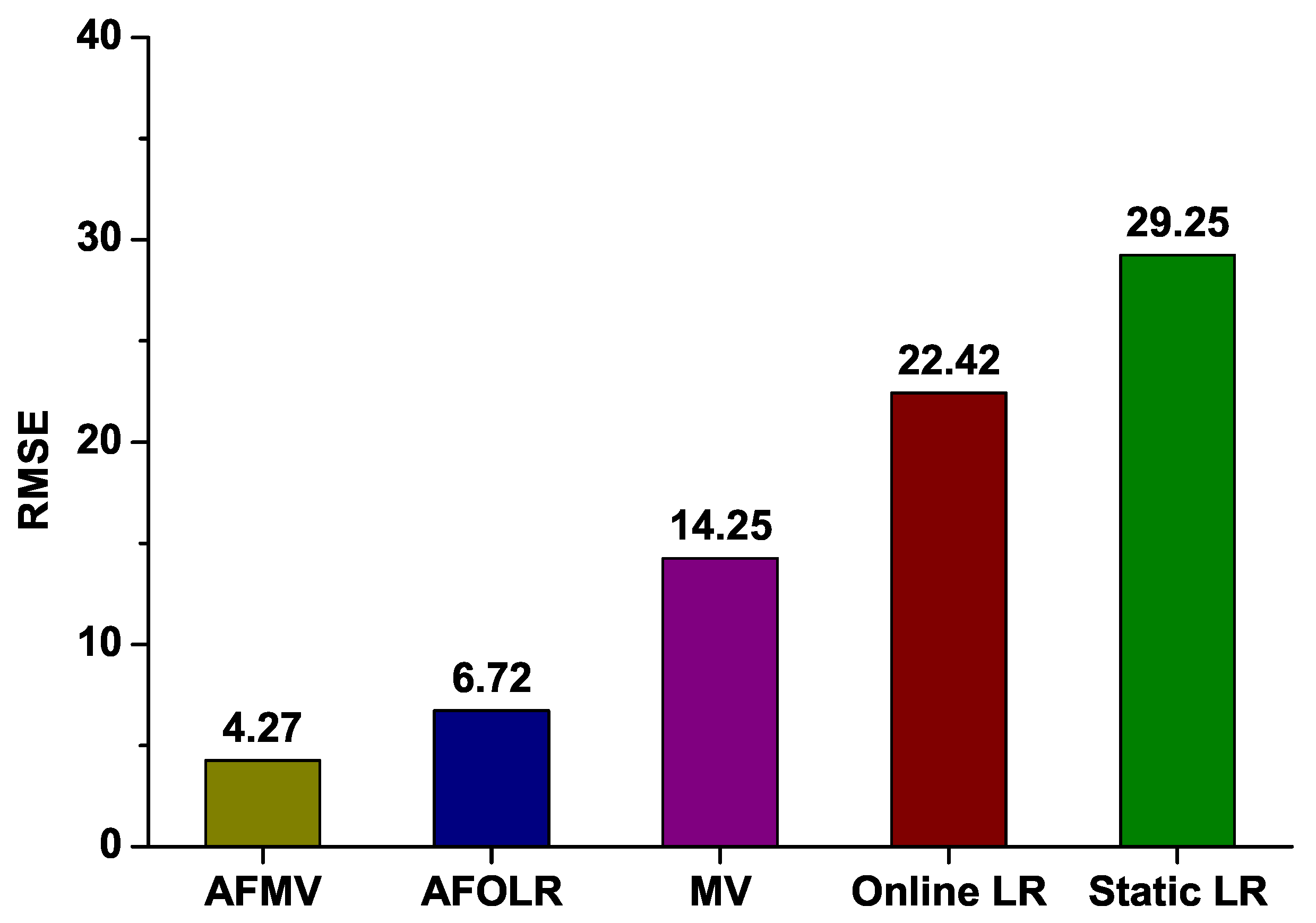
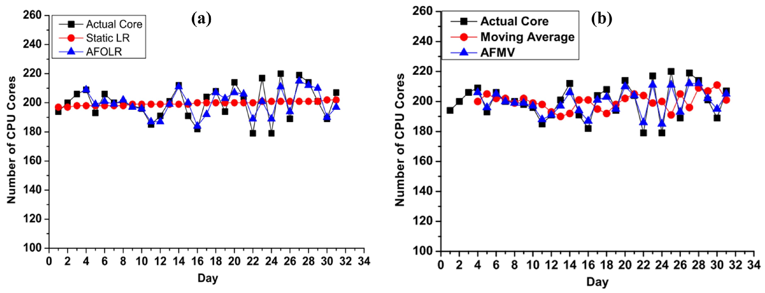
4.1. Quantitative Model Evaluation

In this section, we discuss comparative evaluation results of AFOLR and AFMV schemes with classical linear regression methods and moving average technique. To illustrate quantitative accuracy, we use the Root Mean Squared Error (RMSE) analysis. $RMSE$ can be calculated using following Equation (17) where $Y_t$ is the actual value at time t, $\widehat{Y_t}$ is the predicted one at time t, and p is the number of data points.

$$RMSE=\sqrt{\frac{1}{p}\sum _{t=1}^p{(Y_t-{\widehat{Y}}_t)}^2}$$

(17)

Figure 5 shows evaluation results of five prediction techniques including AFMV, AFOLR, MV, OLR, and standard linear regression LR (depicted as “Static LR”) in terms of $RMSE$. As we can see from the results, our proposed schemes clearly outperform well-known classical forecasting methods. Interestingly, AFMV shows better prediction accuracy than AFOLR since a relatively short interval $(w=5)$ is used for estimation. AFOLR is basically founded on online linear regression which requires more data over a longer period (i.e., larger w) to estimate the coefficient parameters. Nevertheless, both of our proposed methods generate smaller margin of errors compared to the classical regression and moving average techniques.

Figure 5. Root Mean Squared Errors of AFMV, AFOLR, MV, OLR, and Standard Linear Regression.

In order to further investigate the accuracy of our proposed models, we also compared them with the most widely used linear regression and moving average models respectively. Figure 6a presents the comparative analysis of AFOLR model and conventional Linear Regression (Static LR). It shows that distances from actual data (depicted as “Actual Core”) which means the errors of static LR are relatively high and almost move forward statically. On the other hand, our proposed AFOLR scheme can capture the recent trend and predict the data very close to the actual values (“Actual Core” in Figure 6a). This is because it is capable of adapting to recent fluctuations in computing resource availability. Therefore, the AFOLR model clearly outperforms the LR technique and demonstrates its usefulness in predicting even when the datasets are highly variable. We also compared the AFMV approach against a class of time series-based forecasting techniques such as the moving average. The Figure 6b shows a comparison of our AFMV and moving average. Similar to the results of AFOLR in Figure 6a, it is clear that the AFMV model outperforms the traditional moving average, despite the fact that moving average is a well-known approach for predicting in the short term from highly fluctuating data.

Figure 6. Sensitivity Analysis: (a) AFOLR vs. Traditional Linear Regression Technique (Static LR) and (b) AFMV vs. Traditional Moving Average.

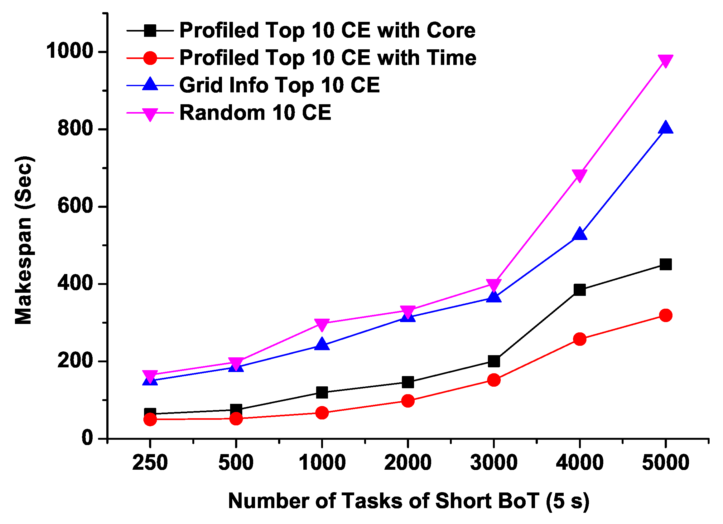
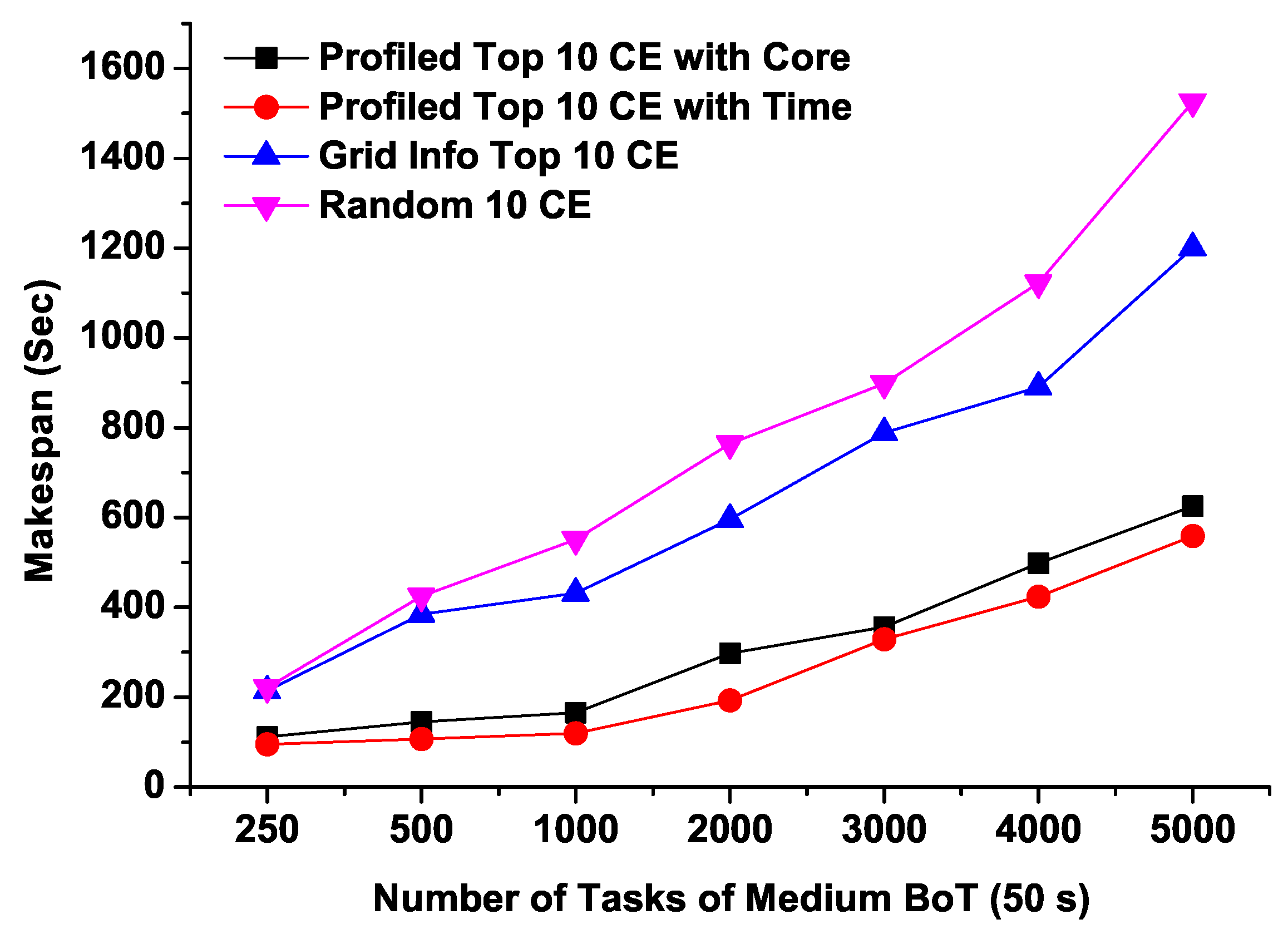
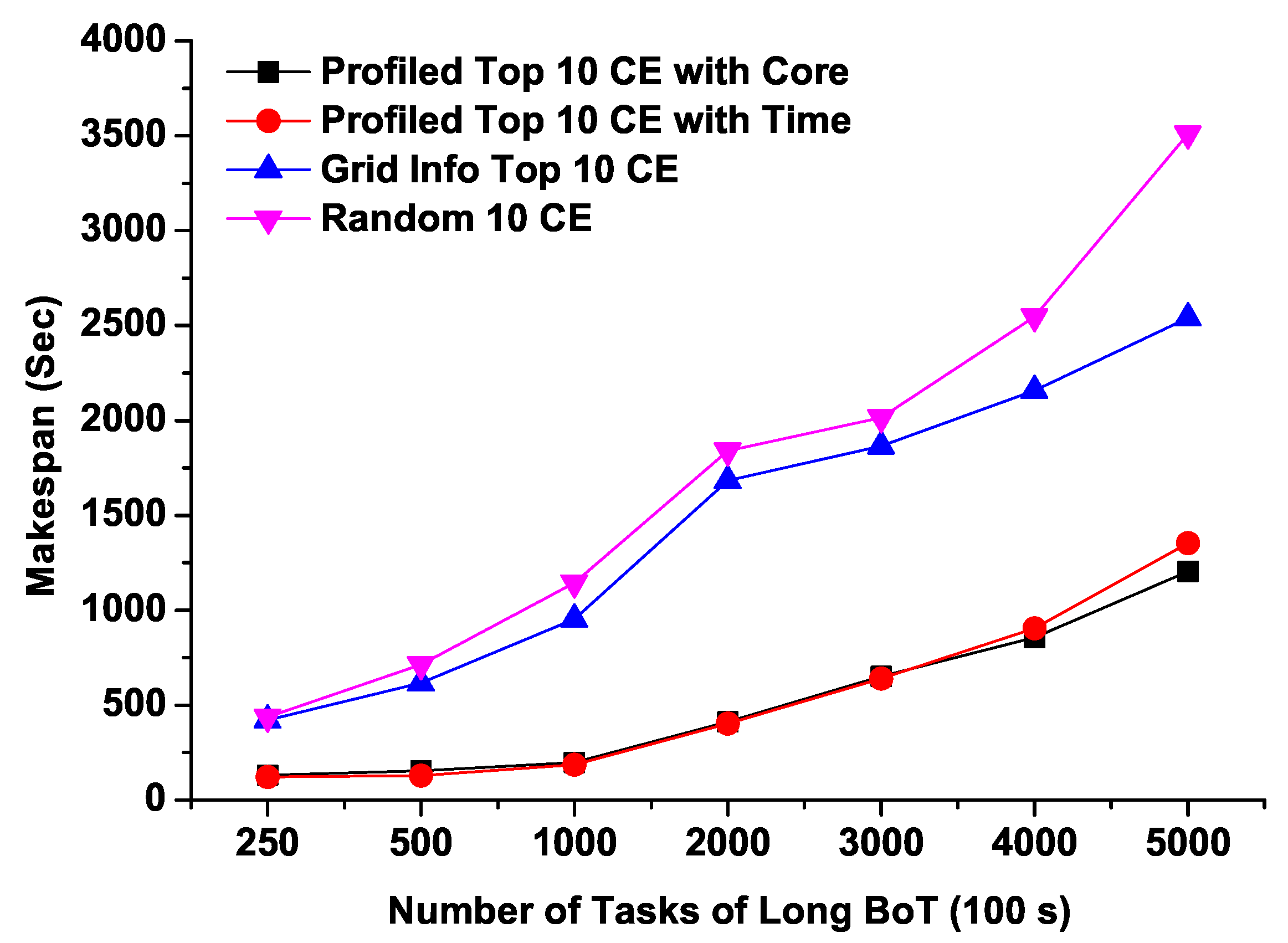
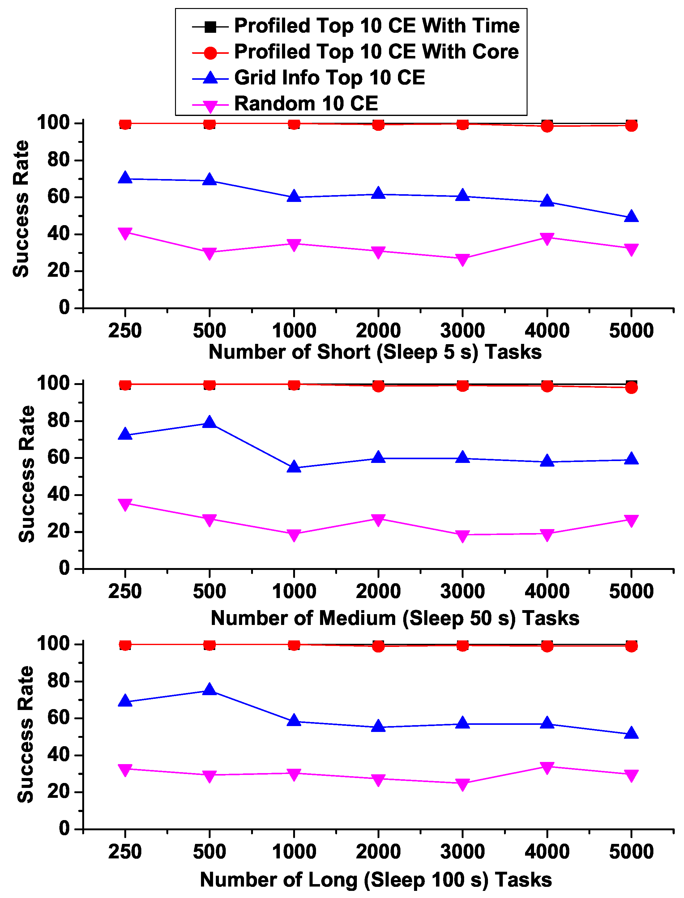
4.2. Microbenchmark Experiments

We also conducted microbenchmark experiments from MTC community [40,41] on the Biomed VO [12] which is a large-scale international and interdisciplinary virtual organization providing tens of thousands of CPU cores to scientific communities. We used three different types of BoT (Bag of Tasks) jobs to evaluate our forecasting model (AFMV) including “Short” (sleep 5 tasks), “Medium” (sleep 50 tasks) and “Long” (sleep 100 tasks) jobs especially from the perspective of Many-Task Computing (MTC) applications [4]. The number of tasks in each BoT job category ranges from 250 to 5000.

In addition, four sets of computing elements (CEs) from Biomed VO with different resource characteristics were selected as followings:

• Profiled Top 10 CE with Core: Top 10 CEs based on model predicted maximum available free CPU cores (i.e., best 10 CEs based on our proposed models that are expected to show maximum number of free CPU cores)
• Profiled Top 10 CE with Time: Top 10 CEs based on model predicted minimum response time (i.e., best 10 CEs based on our proposed model that are expected to show minimum response times)
• Grid Info Top 10 CE: Top 10 CEs based on the number of free CPU cores provided by the Grid Information Service which is an existing conventional monitoring service in VOs.
• Random 10 CE: Randomly selected 10 CEs (i.e., simply a collection of 10 CEs that are randomly selected)

Performance metrics are Makspan and Success Rate. The makspan of a BoT job is defined as the time to complete the execution of all tasks. Success Rate is defined as the ratio of the number of tasks executed successfully to the number of submitted tasks.

Figure 7 shows the Makespans of different sizes of short running BoT jobs with four sets of CEs. Compared to the other three lists of CEs, CEs with the predicted minimum response time (“Profiled Top 10 CE with Time”) can achieve the shortest Makspan. As the number of tasks increases, Makspans of “Grid Info Top 10 CE” and “Random 10 CE” grow rapidly. Interestingly, from these results, we can observe that for short running tasks, expected minimum response time CEs (“Profiled Top 10 CE with Time”) perform better even the “Profiled Top 10 CE with Core” potentially have more free CPU cores.

Figure 7. Makspans of Short BoT jobs with four sets of computing resources.

Figure 8 and Figure 9 illustrate the Makespans of medium and long running BoTs respectively as we increase the number of tasks. It can be noted from Figure 8 that both predicted top 10 CEs (“Profiled Top 10 CE with Time” and “Profiled Top 10 CE with Core”) completed the execution of BoT jobs comparatively within very short time ranging from 100 to 600 s for 250 to 5000 tasks respectively. On the other hand, the job completion time of randomly selected CEs takes about 1600 s for 5000 tasks which is approximately 3 times more than that of profiled CEs based on our proposed model. For the long running BoT jobs, both predicted CEs lists show almost identical performance, however for 5000 tasks, CEs having maximum number of free CPU cores exhibits slightly better turnaround time. From this, it can be arguable that CEs having more free cores can perform better for a large number of tasks having relatively long running times.

Figure 8. Makspans of Medium BoT jobs with four sets of computing resources.

Figure 9. Makspans of Long BoT jobs with four sets of computing resources.

Another important criterion for executing HTC/MTC applications on top of a VO is the Job Completion Rate which refers to the percentage of tasks that can be successfully completed. Figure 10 shows that regardless of task execution times (such as Short, Medium, and Long), both of our predicted Top 10 CEs (“Profiled Top 10 CE with Core” and “Profiled Top 10 CE with Time”) can achieve significantly higher job completion rates than the others. Specifically, both of predicted Top 10 CEs show almost 100% of success rates while “Grid Info Top 10 CE” hovers around 50% to 70%, and “Random 10 CE” shows even worse ranging from 20% to 40%. These results demonstrate that our proposed prediction models can actually improve the user response times and job completion rates for HTC/MTC applications in a real distributed scientific computing environment.

Figure 10. Success Rates of Short, Medium and Long running BoTs.

5. Discussion

Our new adaptive approaches for profiling resource performance-related features (such as the number of available CPU cores and average response times) are based on an effective linear combination of previously collected values and current profiled data. As we can see from the comprehensive experimental results from the Section 4, our proposed schemes have been proved to be effective in a real distributed computing system by significantly improving the overall user response times and job completion rates.

In addition, our quantitative study confirms the efficacy of our profiling methods. Our evaluation findings indicate that our approaches outperform more established statistical models. The comparison of AFOLR with standard linear regression (LR) demonstrates that the distance from real data, which indicates the error of LR, is quite large and virtually marches forward statically. Furthermore, it is clear that the AFMV model is better than the typical moving average, even though the moving average is a well-known method for making short-term forecasts from dynamically changing data

In the future, a multi-objective-based resource profiling approach will undoubtedly increase VOs’ resource utilizations and enable user applications to complete their tasks on time since this technique incorporates many CE performance metrics, including available computing capacity, response time, waiting time, task failure rate, and task resubmission rate, and others. In this regard, fuzzy logic may be advantageous since it is capable of making judgments in an uncertain environment and providing multi-objective solutions [42,43,44]. This study can also point to some new areas to investigate such as developing a novel scheduling method for a resource-shared environment based on resource performance modeling. Finally, we plan to conduct larger-scale mircobenchmark experiments that can consist of millions of tasks and also apply our proposed schemes for real MTC applications (such as drug discovery simulations [45]) in order to further verify the effectiveness of our proposed mechanisms in a real scientific computing environment.

6. Conclusions

Resources in a shared computing environment have varying computing capacity and unreliable performance because of autonomous sharing and control from multiple resource providers. To address this problem, we need to devise effective resource profiling and modeling mechanisms that can periodically collect resource profiling data and predict the future available free resources as well as responsiveness of each computing element based on the profiled data.

In this paper, we presented two novel prediction approaches called AFOLR and AFMV inspired by the concept of difference equation and filtering technique. Comprehensive evaluation results are also presented in terms of quantitative analysis and a large number of microbenchmark tasks. Experimental results show the effectiveness of our proposed prediction models in a real large-scale international and interdisciplinary computing environment. The evaluation results also demonstrate that the proposed models help both the RMS and users in making resource utilization decisions in order to achieve QoS objectives. This study paves the way for future research, such as the development of self-adaptive light-weight filtering approaches to withstand the unpredictable behaviors of resources in shared distributed platforms. Furthermore, future emerging technologies such as Internet of Things (IoT), UAVs, drones, and autonomous driving, which are fundamentally resource-restricted, may be explored to see whether our computationally efficient methods can be applied.

References

1. Xu, L.; Qiao, J.; Lin, S.; Qi, R. Task Assignment Algorithm Based on Trust in Volunteer Computing Platforms. Information 2019, 10, 244. [Google Scholar] [CrossRef]
2. EGI: Advanced Computing for Research. Available online: https://www.egi.eu/ (accessed on 1 December 2021).
3. Rodero, I.; Villegas, D.; Bobroff, N.; Liu, Y.; Fong, L.; Sadjadi, S.M. Enabling interoperability among grid meta-schedulers. J. Grid Comput. 2013, 11, 311–336. [Google Scholar] [CrossRef]
4. Raicu, I.; Foster, I.; Zhao, Y. Many-Task Computing for Grids and Supercomputers. In Proceedings of the Workshop on Many-Task Computing on Grids and Supercomputers (MTAGS’08), Austin, TX, USA, 17 November 2008. [Google Scholar]
5. Raicu, I.; Foster, I.; Wilde, M.; Zhang, Z.; Iskra, K.; Beckman, P.; Zhao, Y.; Szalay, A.; Choudhary, A.; Little, P.; et al. Middleware support for many-task computing. Clust. Comput. 2010, 13, 291–314. [Google Scholar] [CrossRef]
6. Field, L.; Spiga, D.; Reid, I.; Riahi, H.; Cristella, L. CMS@ home: Integrating the Volunteer Cloud and High-Throughput Computing. Comput. Softw. Big Sci. 2018, 2, 2. [Google Scholar] [CrossRef]
7. Anderson, D.P. BOINC: A platform for volunteer computing. J. Grid Comput. 2019, 18, 99–122. [Google Scholar] [CrossRef]
8. Sanjay, H.; Vadhiyar, S. Performance modeling of parallel applications for grid scheduling. J. Parallel Distrib. Comput. 2008, 68, 1135–1145. [Google Scholar] [CrossRef]
9. Qureshi, M.B.; Dehnavi, M.M.; Min-Allah, N.; Qureshi, M.S.; Hussain, H.; Rentifis, I.; Tziritas, N.; Loukopoulos, T.; Khan, S.U.; Xu, C.Z.; et al. Survey on grid resource allocation mechanisms. J. Grid Comput. 2014, 12, 399–441. [Google Scholar] [CrossRef]
10. Hossain, M.A.; Vu, H.T.; Kim, J.S.; Lee, M.; Hwang, S. SCOUT: A Monitor and Profiler of Grid Resources for Large-Scale Scientific Computing. In Proceedings of the 2015 International Conference on Cloud and Autonomic Computing (ICCAC), Boston, MA, USA, 21–25 September 2015; pp. 260–267. [Google Scholar]
11. Hossain, M.A.; Nguyen, C.N.; Kim, J.S.; Hwang, S. Exploiting resource profiling mechanism for large-scale scientific computing on grids. Clust. Comput. 2016, 19, 1527–1539. [Google Scholar] [CrossRef]
12. The Biomed Virtual Organization. Available online: http://lsgc.org/biomed.html (accessed on 17 December 2021).
13. Entezari-Maleki, R.; Trivedi, K.S.; Movaghar, A. Performability evaluation of grid environments using stochastic reward nets. IEEE Trans. Dependable Secur. Comput. 2014, 12, 204–216. [Google Scholar] [CrossRef]
14. Forestiero, A.; Mastroianni, C.; Spezzano, G. A Multi-agent Approach for the Construction of a Peer-to-Peer Information System in Grids. In Self-Organization and Autonomic Informatics (I); IOS Press: Amsterdam, The Netherlands, 2005. [Google Scholar]
15. Ramachandran, K.; Lutfiyya, H.; Perry, M. Decentralized resource availability prediction for a desktop grid. In Proceedings of the 2010 10th IEEE/ACM International Conference on Cluster, Cloud and Grid Computing (CCGrid), Melbourne, Australia, 17–20 May 2010; pp. 643–648. [Google Scholar]
16. Shariffdeen, R.; Munasinghe, D.; Bhathiya, H.; Bandara, U.; Bandara, H.D. Adaptive workload prediction for proactive auto scaling in PaaS systems. In Proceedings of the 2016 2nd International Conference on Cloud Computing Technologies and Applications (CloudTech), Marrakech, Morocco, 24–26 May 2016; pp. 22–29. [Google Scholar]
17. Smith, W.; Foster, I.; Taylor, V. Predicting application run times with historical information. J. Parallel Distrib. Comput. 2004, 64, 1007–1016. [Google Scholar] [CrossRef]
18. Seneviratne, S.; De Silva, L.C.; Witharana, S. Taxonomy and Survey of Performance Prediction Systems for the Distributed Systems Including the Clouds. In Proceedings of the 2021 IEEE International Conferences on Internet of Things (iThings) and IEEE Green Computing & Communications (GreenCom) and IEEE Cyber, Physical & Social Computing (CPSCom) and IEEE Smart Data (SmartData) and IEEE Congress on Cybermatics (Cybermatics), Melbourne, Australia, 6–8 December 2021; pp. 262–268. [Google Scholar]
19. Seneviratne, S.; Witharana, S.; Toosi, A.N. Adapting the machine learning grid prediction models for forecasting of resources on the clouds. In Proceedings of the 2019 Advances in Science and Engineering Technology International Conferences (ASET), Dubai, United Arab Emirates, 26 March–10 April 2019; pp. 1–6. [Google Scholar]
20. Dinda, P.A.; O’hallaron, D.R. Host load prediction using linear models. Clust. Comput. 2000, 3, 265–280. [Google Scholar] [CrossRef]
21. Javadi, B.; Kondo, D.; Vincent, J.M.; Anderson, D.P. Discovering statistical models of availability in large distributed systems: An empirical study of seti@ home. IEEE Trans. Parallel Distrib. Syst. 2011, 22, 1896–1903. [Google Scholar] [CrossRef]
22. Anderson, D.P.; Cobb, J.; Korpela, E.; Lebofsky, M.; Werthimer, D. SETI@home: An Experiment in Public-Resource Computing. Commun. ACM 2002, 45, 56–61. [Google Scholar] [CrossRef]
23. Padhye, V.; Tripathi, A. Resource Availability Characteristicsand Node Selection in CooperativelyShared Computing Platforms. IEEE Trans. Parallel Distrib. Syst. 2014, 25, 1044–1054. [Google Scholar] [CrossRef][Green Version]
24. PlanetLab: An Open Platform for Developing, Deploying, and Accessing Planetary-Scale Services. Available online: https://www.planet-lab.org/ (accessed on 3 December 2021).
25. Rood, B.; Lewis, M.J. Grid resource availability prediction-based scheduling and task replication. J. Grid Comput. 2009, 7, 479–500. [Google Scholar] [CrossRef]
26. Wolski, R.; Spring, N.T.; Hayes, J. The network weather service: A distributed resource performance forecasting service for metacomputing. Future Gener. Comput. Syst. 1999, 15, 757–768. [Google Scholar] [CrossRef]
27. Verma, M.; Gangadharan, G.; Narendra, N.C.; Vadlamani, R.; Inamdar, V.; Ramachandran, L.; Calheiros, R.N.; Buyya, R. Dynamic resource demand prediction and allocation in multi-tenant service clouds. Concurr. Comput. Pract. Exp. 2016, 28, 4429–4442. [Google Scholar] [CrossRef]
28. Cameron, D.; Casey, J.; Guy, L.; Kunszt, P.; Lemaitre, S.; McCance, G.; Stockinger, H.; Stockinger, K.; Andronico, G.; Bell, W.; et al. Replica management services in the european datagrid project. In Proceedings of the UK e-Science All Hands Meeting 2004, Nottingham UK, 31 August–3 September 2004. [Google Scholar]
29. Faerman, M.; Su, A.; Wolski, R.; Berman, F. Adaptive performance prediction for distributed data-intensive applications. In Proceedings of the 1999 ACM/IEEE Conference on Supercomputing, Portland, OR, USA, 13–19 November 1999; p. 36-es. [Google Scholar]
30. Nudd, G.R.; Kerbyson, D.J.; Papaefstathiou, E.; Perry, S.C.; Harper, J.S.; Wilcox, D.V. PACE—A toolset for the performance prediction of parallel and distributed systems. Int. J. High Perform. Comput. Appl. 2000, 14, 228–251. [Google Scholar] [CrossRef]
31. Desprez, F.; Quinson, M.; Suter, F. Dynamic Performance Forecasting for Network-Enabled Servers in a Heterogeneous Environment. Ph.D. Thesis, INRIA, Le Chesnay-Rocquencourt, France, 2001. [Google Scholar]
32. Kumar, J.; Singh, A.K. Workload prediction in cloud using artificial neural network and adaptive differential evolution. Future Gener. Comput. Syst. 2018, 81, 41–52. [Google Scholar] [CrossRef]
33. Bi, J.; Li, S.; Yuan, H.; Zhou, M. Integrated deep learning method for workload and resource prediction in cloud systems. Neurocomputing 2021, 424, 35–48. [Google Scholar] [CrossRef]
34. Song, B.; Yu, Y.; Zhou, Y.; Wang, Z.; Du, S. Host load prediction with long short-term memory in cloud computing. J. Supercomput. 2018, 74, 6554–6568. [Google Scholar] [CrossRef]
35. Gul, F.; Mir, I.; Abualigah, L.; Sumari, P.; Forestiero, A. A Consolidated Review of Path Planning and Optimization Techniques: Technical Perspectives and Future Directions. Electronics 2021, 10, 2250. [Google Scholar] [CrossRef]
36. Hellerstein, J.L.; Diao, Y.; Parekh, S.; Tilbury, D.M. Feedback Control of Computing Systems; Wiley Online Library: Hoboken, NJ, USA, 2004. [Google Scholar]
37. Rho, S.; Kim, S.; Kim, S.; Kim, S.; Kim, J.S.; Hwang, S. HTCaaS: A Large-Scale High-Throughput Computing by Leveraging Grids, Supercomputers and Cloud. In Proceedings of the Research Poster at IEEE/ACM International Conference for High Performance Computing, Networking, Storage and Analysis (SC12), Salt Lake City, UT, USA, 10–16 November 2012. [Google Scholar]
38. Kim, J.S.; Rho, S.; Kim, S.; Kim, S.; Kim, S.; Hwang, S. HTCaaS: Leveraging Distributed Supercomputing Infrastructures for Large-Scale Scientific Computing. In Proceedings of the 6th ACM Workshop on Many-Task Computing on Clouds, Grids, and Supercomputers (MTAGS’13) Held with SC13, San Francisco, CA, USA, 2–7 July 2013. [Google Scholar]
39. Rawlings, J.O.; Pantula, S.G.; Dickey, D.A. Applied Regression Analysis: A Research Tool; Springer Science & Business Media: Berlin/Heidelberg, Germany, 2001. [Google Scholar]
40. Raicu, I.; Zhao, Y.; Dumitrescu, C.; Foster, I.; Wilde, M. Falkon: A Fast and Light-weight tasK executiON framework. In Proceedings of the 2007 ACM/IEEE conference on Supercomputing (SC’07), Reno, NV, USA, 10–16 November 2007. [Google Scholar]
41. Raicu, I.; Zhang, Z.; Wilde, M.; Foster, I.; Beckman, P.; Iskra, K.; Clifford, B. Towards Loosely-Coupled Programming on Petascale Systems. In Proceedings of the 2008 ACM/IEEE conference on Supercomputing (SC’08), Austin, TX, USA, 15–21 November 2008. [Google Scholar]
42. Tchier, F.; Ali, G.; Gulzar, M.; Pamučar, D.; Ghorai, G. A New Group Decision-Making Technique under Picture Fuzzy Soft Expert Information. Entropy 2021, 23, 1176. [Google Scholar] [CrossRef] [PubMed]
43. Ali, G.; Ansari, M.N. Multiattribute decision-making under Fermatean fuzzy bipolar soft framework. Granul. Comput. 2022, 7, 337–352. [Google Scholar] [CrossRef]
44. Ali, G.; Alolaiyan, H.; Pamučar, D.; Asif, M.; Lateef, N. A novel MADM framework under q-rung orthopair fuzzy bipolar soft sets. Mathematics 2021, 9, 2163. [Google Scholar] [CrossRef]
45. Rao, V.S.; Srinivas, K. Modern drug discovery process: An in silico approach. J. Bioinform. Seq. Anal. 2011, 2, 89–94. [Google Scholar]
Publisher’s Note: MDPI stays neutral with regard to jurisdictional claims in published maps and institutional affiliations.
Article Metrics
Citations
Article Access Statistics
Multiple requests from the same IP address are counted as one view.