Bending Behavior of a Frictional Single-Layered Spiral Strand Subjected to Multi-Axial Loads: Numerical and Experimental Investigation

Abstract

Bending deformation gives rise to interwire slippage for spiral strands subjected to multi-axial loads, and further induces wear or fatigue phenomena in practice. The interwire friction would resist bending deformation and lead to uneven tension distribution of individual constituent wires but little research has quantified these effects. To figure out this issue, a beam finite element (FE) is established, into which a penalty stiffness algorithm and a Coulomb friction model are incorporated. A series of free bending simulations are developed for parametric study on deflection near the terminations and tension distribution of individual wire for strands with different levels of length and friction coefficient as well as external loads. Based on the simulation results, it is found that strand length has little influence on bending deformation and tension distribution if the strand length exceeds six times the pitch length. A deflection formula extended from the classical Euler beam model well predicts the sag deflections and the relative error with respect to experimental measurements is less than 10%. Furthermore, additional axial tension induced by the friction is clearly characterized and an approximate expression is proposed to estimate tension distribution for outer layer wires. Its predictions are encouraging for longer strands.

1. Introduction

A spiral strand is a composite structure that consists of helical wires twisted around an initially straight core and grouped in concentric layers; it is a critical component of cable structure or wire rope. The helical structures are widely applied for long-distance force delivery or signal transmission in many engineering applications, such as suspension cables in cable-stayed bridges and electrical conductors as well as wire rope in mining hoists. These structures are mainly designed for bearing axial loads, but they inevitably experience bending deformations and/or transverse vibrations caused by the gravity, hanging, or wind disturbance in practice. In these cases, bending stiffness is an essential parameter for the estimation of lateral deformation near the terminations or transverse vibration with high-order nature frequencies. For instance, neglecting bending stiffness will lead to unacceptable errors in the estimation of high-order nature frequencies for large-diameter sag cables experiencing transverse vibration [1]. Moreover, cyclic bending is a vital factor in fretting fatigue damage which happens at or near the terminations where the strand curvature rapidly changes. Although the bending stiffness of cables is small, it has a large influence on the deformed shape near the constraints [2,3]. In addition, flexural hysteresis damping properties play an important role in dynamic behaviors [4], and flexural self-damping depends on the nonlinear hysteresis bending stiffness [5]. However, the spiral strand exhibits extremely complicated bending behavior because of intractable interaction in the strand. In fact, the bending stiffness for spiral strands may vary with their tension, curvature and deformation history [6]. Therefore, accurately characterizing the effect of friction on the bending behaviors of spiral strands is essential for dynamic analysis, fatigue life prediction and self-damping estimation.

Earlier studies on the bending behaviors of spiral strands mainly focus on experimental measurements, and a direct and effective experimental approach is to measure the deflection of spiral strands subjected to external loads under free bending. McConnell and Zemke [7] measured the flexural stiffness of multistrand electrical conductors under tension, and they found that the bending stiffness increased with tension. Similarly, Filiatrault and Christopher [8] pointed out that the bending stiffness of two electrical conductors approach minimum theoretical bending stiffness under most combinations of axial tension and lateral deformation. However, for very large axial tension, the bending stiffness is closer to the maximum possible bending stiffness. Apart from electrical conductors, sag deflections for several structural cables are also measured by Chen et al. [9]. These tests showed elastic-plastic like force-displacement responses under bending. However, the experimental method costs huge human efforts and financial resources. Additionally, the effective bending stiffness is derived based on the assumption that the bending stiffness is constant along the strand centerline, but this is not consistent with the realistic one.

To avoid the drawbacks of experimental methods, many researchers have tried to derive the bending deformation of spiral strands based on mechanical principles. A discrete model which consists of six nonlinear differential equations of equilibrium is derived based on Love’s thin rod theory [10]. Costello [11] proposed a formula for the minimum bending stiffness by treating the spiral strand as an assembly of individual helical springs. Cao and Wu [12] put forward a change law of the secondary helix angle and established a new mechanical model for a multi-strand wire rope under a bending state. However, the inner friction was ignored. Later on, several mechanical models were proposed to evaluate the impact of friction on the bending behavior. Under the assumption that no slippage exists in the strand, LeClair and Costello [13] predicted the stresses and contact forces in a single-layered strand subjected to axial, bending and torsional loading. Chen et al. [14] established a semi-analytical model for a spiral strand subjected to bending load, in which interwire contact deformation and the effects of Poisson’s ratio were considered. However, the assumption adopted might be questionable, and as indicated by Ramsey [15] the constituent wires of the spiral strand exhibit a strong tendency to rotate with respect to one another in a practical situation of bending deformation of spiral strands. Except for the discrete model, another different semi-continuous model, in which each layer of a strand is modeled as a combination of concentric orthotropic cylinders, is presented to deal with the tensile, torsional and bending stiffness of multi-layered strands [16,17].

To more accurately characterize the bending behavior of spiral strands, the wire slippage criterion should be introduced to link the friction on the contact interface and the internal axial tension of the constituent wires. The relationship between the moment and the associated curvature was determined in [18] and the bending deformation process was divided into three stages. Lanteigne [19] determined the wire’s axial force of multi-layered strand based on the Bernoulli–Euler beam assumption, and the diminishing of the bending stiffness caused by the interlayer slippage is involved. Later on, an instructive slippage criterion governing the relationship between the axial force and friction was proposed by Papailiou [20]. This slippage criterion is widely accepted as it is consistent with the observation in the fatigue experiment carried out by Hobbs and Ghavami [21] that the first failed wire is invariably located near the bending neutral axis rather than the wires in the extreme-fiber position. In 2005, Hong et al. [22] extended Papailiou’s theoretical model into multilayered strands by considering the transmission of hoop force induced by axial tension from the outer-layer to the inner-layer. Recently, Foti and Martinelli [23,24] presented a refined mechanical description for metallic strands and a hysteretic moment−curvature relationship was accounted for. Similarly, Khan et al. [25] developed a new analytical formulation to predict the bending stiffness for multi-layered spiral strands by considering wire-wire line contact in the same layer and contact deformation. Zheng et al. [26] presented a nonlinear bending stiffness for multi-layered strands by considering the wire slippage delayed by bending load.

With the rapid development of computation capability, more and more research focuses on finite element (FE) analysis of the bending behavior of spiral strands. Compared with the analytical method, the FE method is of the capability to capture the realistic inter-wire slippage and interaction inside the spiral strand without any assumptions. Nawrocki and Labrosse [27] adopted the FE method to study the interwire motions of a simple spiral strand subjected to axial loadings and bending deformations. Later on, with the aid of the commercial FE software, several researchers investigated the mechanical behavior and stress distribution of various types of spiral strands. According to the basic elements implemented in different FE models, they can be categorized into four types, involving a full three dimensional (3D) solid model [28,29,30,31,32,33,34], a solid-beam mixed model [35], a beam-spring mixed model [36] and a beam model [37,38,39,40,41]. In the full 3D FE model, each constituent wire of the spiral strand is discretized with hexahedral solid elements and nonlinear properties, such as frictional contact or elastoplastic constitutive material model can be introduced to the model. Yu et al. [28] examined the bending behavior and interface stress distributions for a simple strand under longitudinal and lateral loadings. Judge et al. [29] predicted the axial load-strain curves and failure loads for two types of spiral strand cables which were in good agreement with experimental data. Kmet et al. [30] analyzed the stress distribution of a four-layered spiral strand bent over a curved support. Similarly, Xing and Zhou [31] studied the bending behavior of a simple strand with different layer angles and coefficients of friction under zero tension. Zhang and Martin [32] investigated the bending stiffness for a preloaded single-layered strand with friction. In order to reduce the computational magnitude inherent to the full 3D FE model, Jiang et al. [33,34] built a concise finite element model for a simple wire strand with 1/6 pitch length for bending and another FE model for a three-layered strand for axial stretching according to the periodic and axisymmetric structure in the axial and circumferential direction, respectively. However, it is still worth noting that full 3D FE models suffer from huge computational costs and are time consuming, especially for spiral strands with long lengths or complex geometry. To overcome these drawbacks, several researchers have proposed some substitution models in which solid elements are replaced by more effective beam elements. Kim and Lee [35] built a mixed solid-beam element model to analyze the mechanical behavior of helically stranded cables under axial and transverse loads. Compared with the solid model, the mixed model possesses high accuracy and significantly low computational cost. For the same reason, Yu et al. [36] established a mixed beam-spring element model to simulate the quasi-static bending process for structural cables on the commercial software platform ANSYS. This model incorporates user defined triaxial springs to simulate the contact extrusion and friction resistance. Similarly, Zhou and Tian [37] presented a beam FE model to simulate pure stretching and bending for a simple strand. S. Lalonde et al. [38] also developed a beam FE model into which the beam-to-beam contact algorithm and a multi-level Coulomb friction model were incorporated to deal with the interwire contact and friction forces for multi-layered strands under multiaxial loads. Recently, Rezaiee-Pajand et al. [39,40,41] developed a curved beam to improve efficiency and accuracy with fewer numbers of beam elements.

Nevertheless, previous studies seldom conduct parametric analysis to quantify the effects of friction on the bending deformation and tension distribution for spiral strands. In addition, the bending mechanism near the terminations is never examined for strands with different lengths. Therefore, this work is mainly intended to figure out the effects of friction on the bending behaviors of a single-layered strand with different lengths and subjected to multi-axial loads. This paper is organized as follows: In Section 2, a beam FE modeling strategy and data fitting methodology were presented in detail. In addition, an experiment was carried out to validate the beam FE model. In Section 3, a parametric study and comparative study were developed to validate the proposed formulas.

2. Materials and Methods

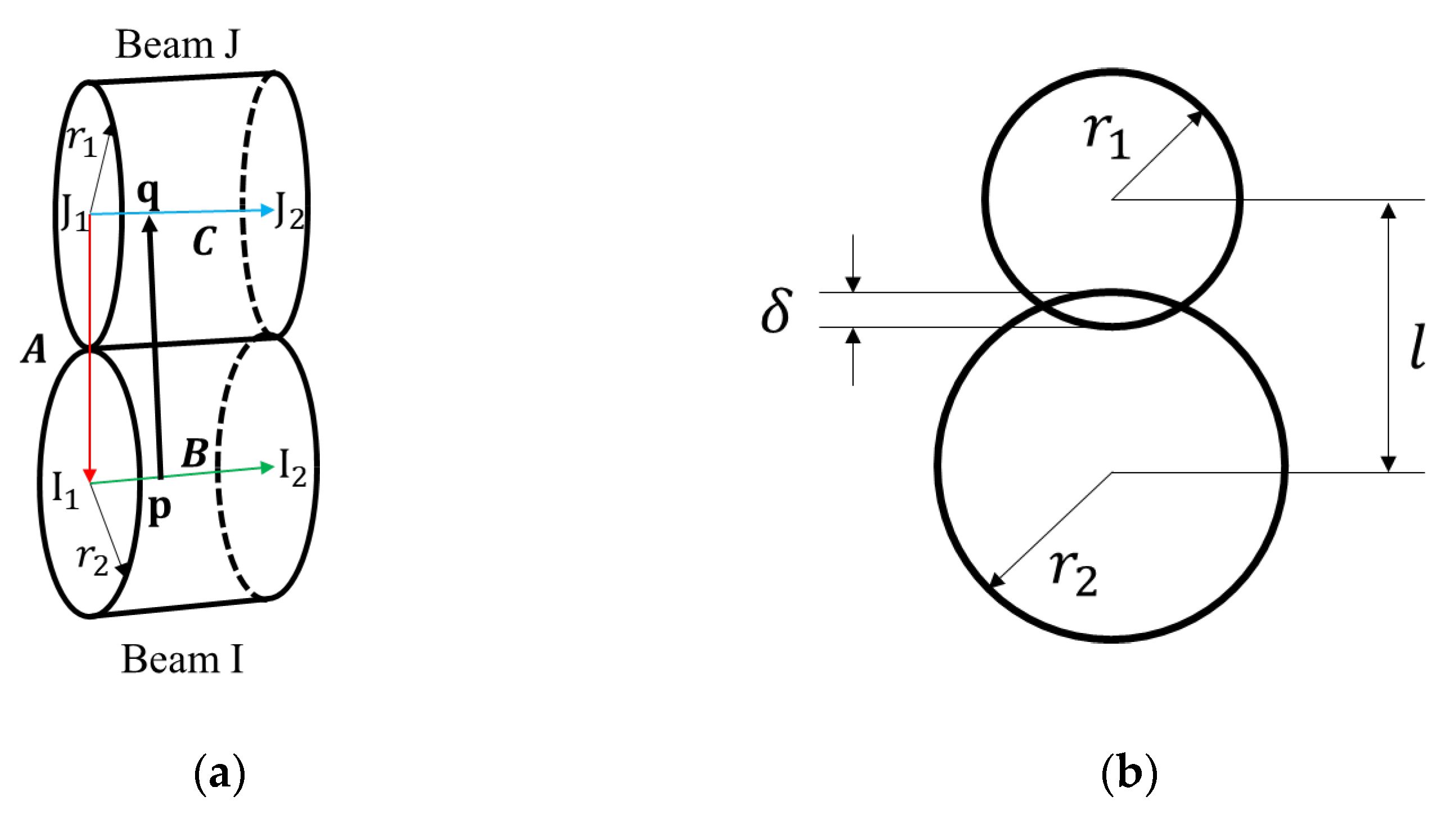
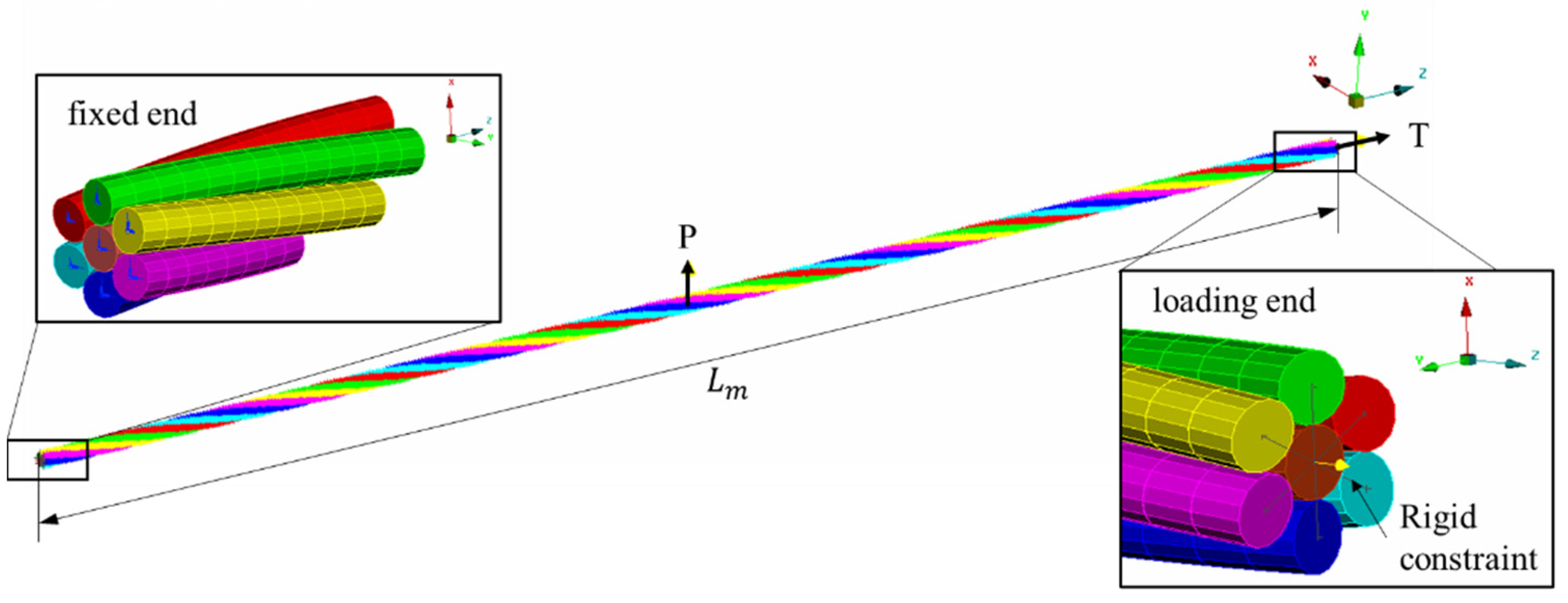
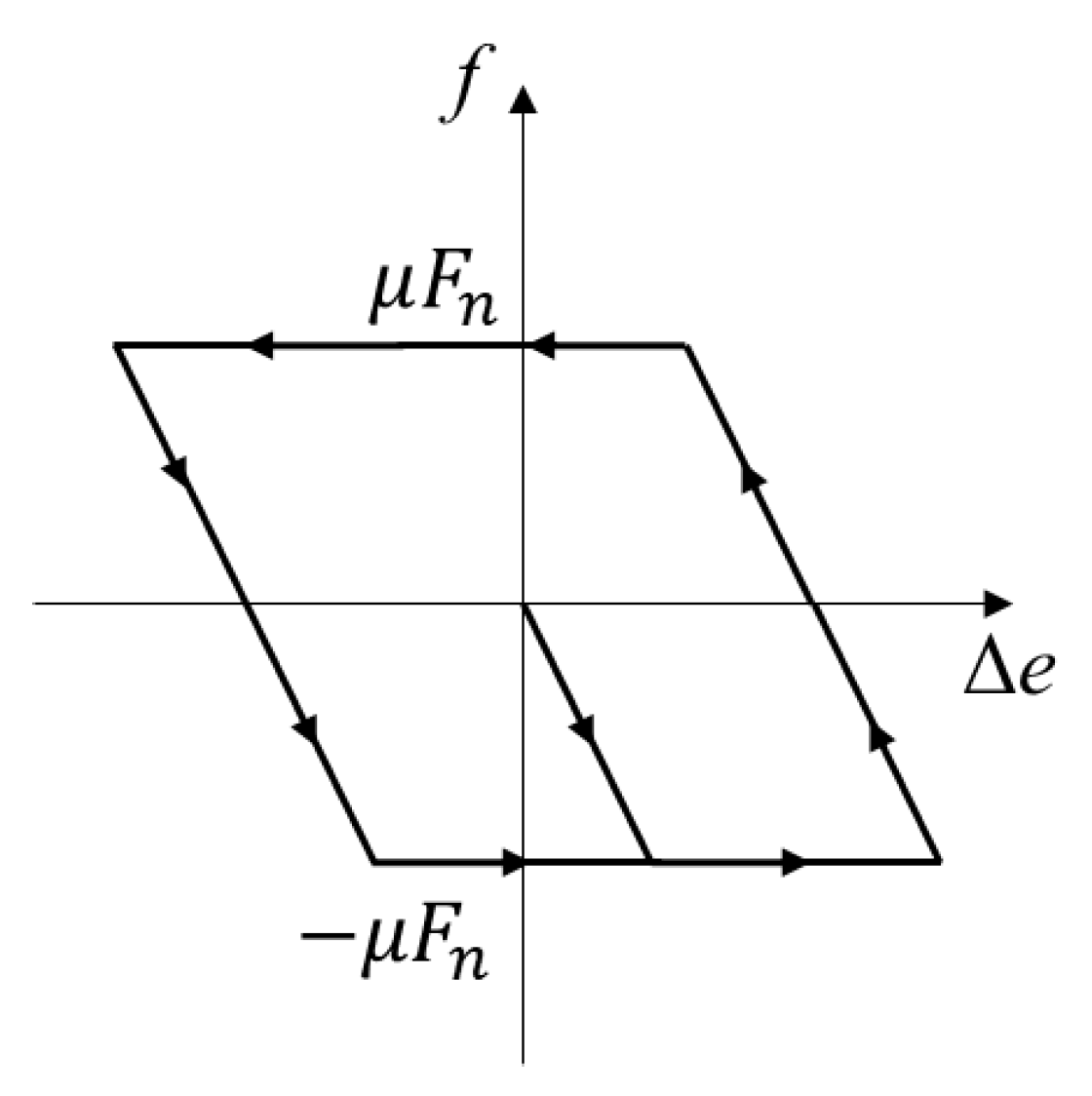
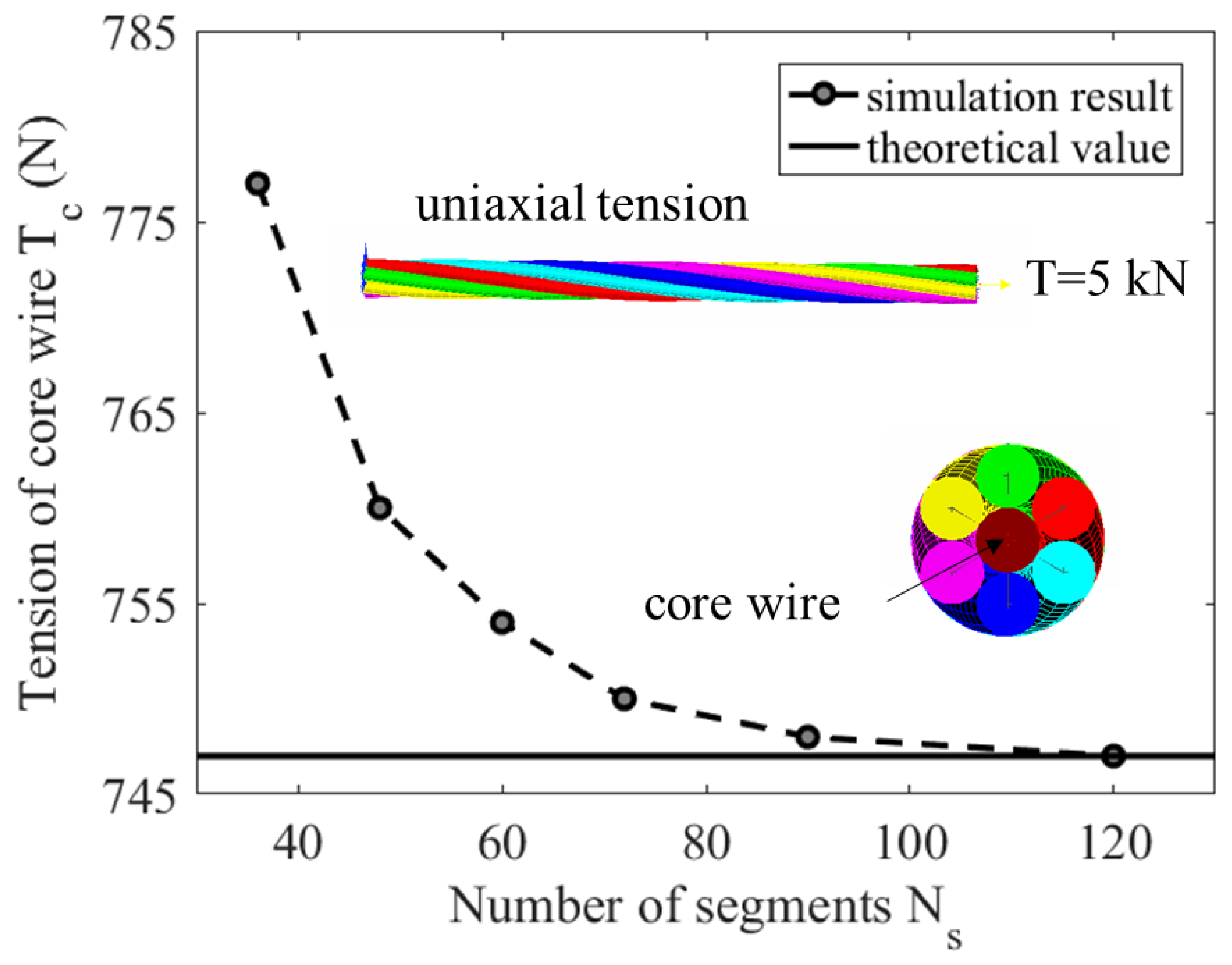
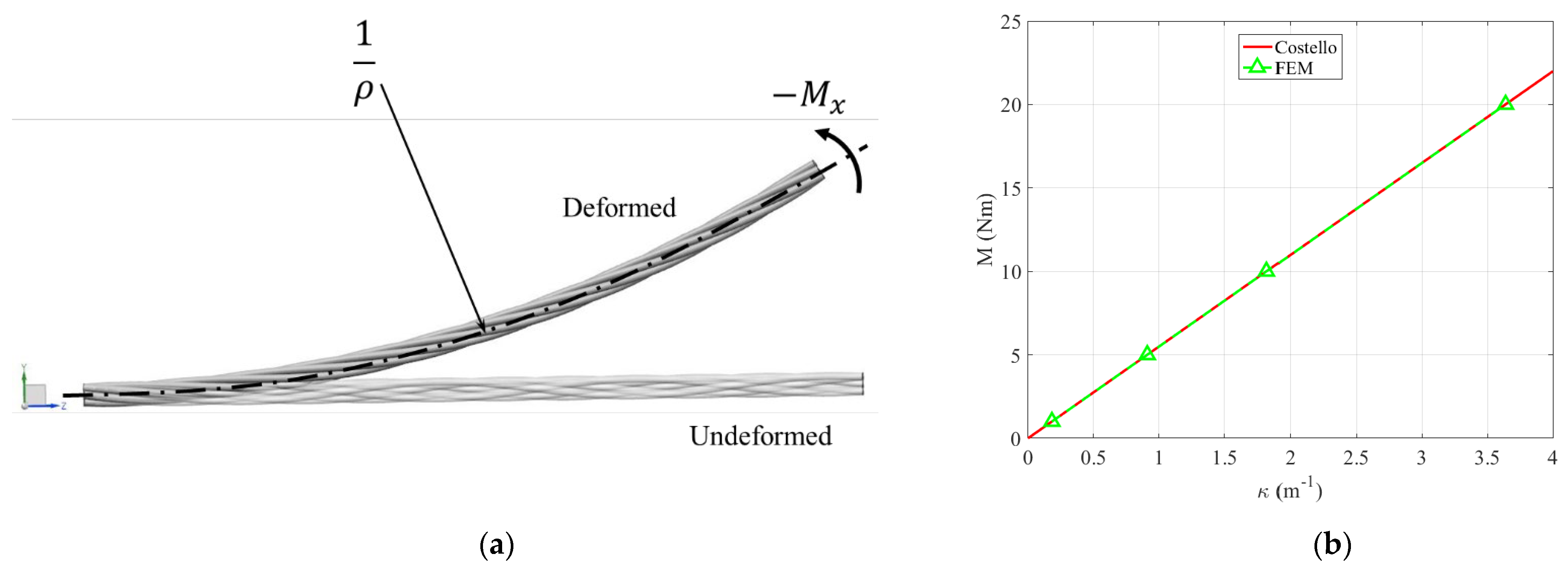
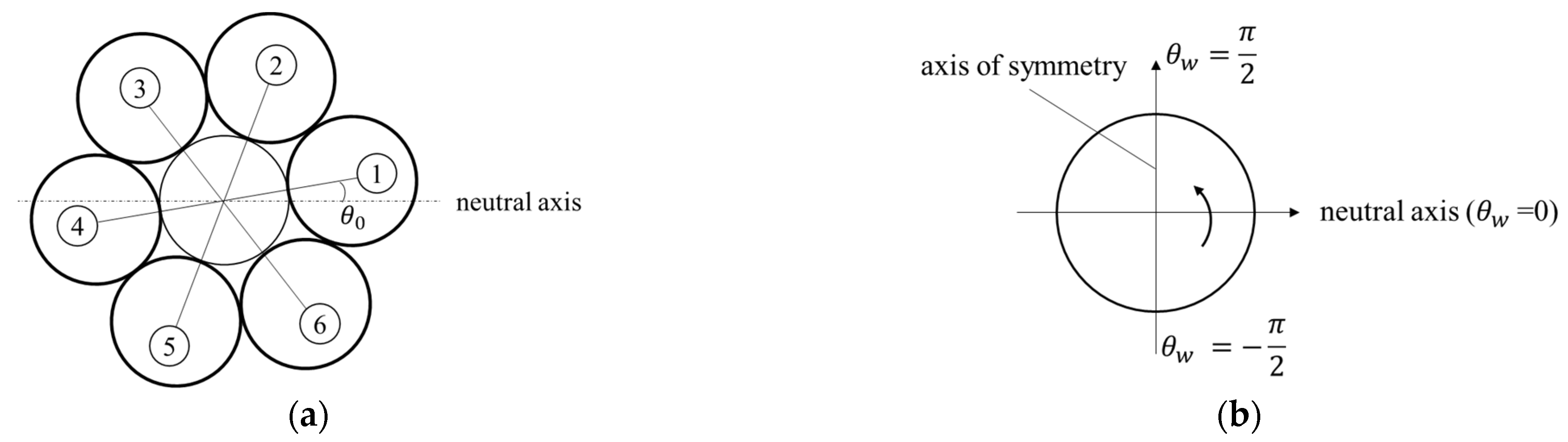
2.1. A Beam FE Modeling Strategy for a Simple Strand under Multi-Axial Loads

A simple strand, also namely 1 + 6 steel strand, consists of one straight core and six outer layered wires wound around the core, as shown in Figure 1. The geometry of the strand is characterized as follows: the radius of the core is R_c, the radius of the outer layered wire is R_w, and the layer angle is α. Here, the layer angle is defined as the included angle between the centerline of the outside wire and that of the core wire.

The centerline of the outer wire is a first-order helical curve characterized by helical radius R_h and pitch length p. The pitch length is defined as the distance between two nodes situated on the helical wire whose corresponding angular phases differ by 2π along the longitudinal axis of the strand. The parametrical equation of the helical curve is expressed as:

$$\mathit{R}=\left[R_h\cos \theta ,R_h\sin \theta ,\frac{p}{2\pi }\theta \right]$$

(1)

According to geometrical relations, there exists:

$$R_h=R_c+R_w$$

(2)

and the pitch length:

$$p=2\pi R_h\tan \beta$$

(3)

where $\beta$ represents the helical angle of the helical curve and $\beta =\frac{\pi }{2}-\alpha .$

All necessary parameters involving geometric dimensions and material properties of the simple strand are listed in

Table 1. Properties of the simple strand.

Symbol	Physical Meaning	Value
Rc	Radius of core wire	1.52 mm
Rw	Radius of outer wire	1.50 mm
p	Pitch length	141.58 mm
α	Layer angle	0.1331 rad
m	Number of outer wires	6
E	Youngs modulus	197,950 MPa
ν	Poisson ratio	0.3

. Note, that only the elasticity phase of steel is considered here due to the assumption of the small strain of the spiral strand under free bending. Additionally, both radial and circumferential contact exists in the present strand.

A 2-node Hughes–Liu beam element [42] implemented in Ls-dyna is utilized to generate a FE model for investigating bending behaviors of the simple strand. For each node of the beam element, there are 6 degrees of freedom in total involving 3 translational and 3 rotational degrees of freedom This beam element has high computational efficiency and good robustness. In addition, it has no locking modes because the integral algorithm of the beam element is performed with one-point integration along the axis and multiple points in the cross section. Therefore, it can be utilized to deal with the finite strains that occur in many practical applications.

To capture the interaction of the adjacent wires in the strand in the process of deformation, a typical penalty stiffness algorithm is applied to evaluate the normal contact force on the interface. As shown in Figure 2, once the beam element I and the beam element J contact with a so-called penetration δ, the penalty stiffness spring will generate a penalty force to eliminate the penetration.

Assuming the radius of two beam elements are $r_1$ and $r_2$, respectively, and the distance between their cross-sectional centers is l, the contact penetration δ can be calculated by:

$$\delta =r_1+r_2-l$$

(4)

The distance of two adjacent beams is obtained through vector operation

$$l=\parallel \frac{\mathit{A}\cdot \left(\mathit{B}\times \mathit{C}\right)}{\mathit{B}\times \mathit{C}}\parallel$$

(5)

Here, A denotes the vector pointing from node I₁ to J₁, B denotes the vector pointing from node I₁ to I₂, and C denotes the vector pointing from node J₁ to J₂. I₁ and I₂ are two nodes of beam I, and J₁ and J₁ are two nodes of beam J.

According to the penalty stiffness algorithm, the normal contact force of two adjacent beam elements holds:

$$F_n=k^{*}\delta$$

(6)

$k^{*}$ represents the integrated interface contact stiffness. Its magnitude depends on the contact stiffness of two contacting beam elements, and there exists:

$$k^{*}=\frac{k_i{k}_j}{k_i+k_j}$$

(7)

where $k_i$ and $k_j$ is the contact stiffness of beam I and beam J, respectively.

The contact stiffness of a beam element is related to its material properties and geometric parameters and it can be calculated by:

$$k=\frac{f_s\pi K{R}^2}{L}$$

(8)

where $K$ is the Bulk modulus and $K=\frac{E}{3\left(1-2\nu \right)}$, $f_s$ is the scale factor and the default value is 0.1, $R$ is the radius of the beam element and L is the beam element length.

A Coulomb friction model, which is analogous to an elastic-plastic spring, is adopted to evaluate the friction which resists the relative movement between two contacting beams. The incremental update algorithm is more convenient to describe the friction model since it is path dependent. Figure 3 shows that the friction varies with the relative displacement $\mathsf{\Delta }e$ perpendicular to the normal contact force between two contacting beams.

Assuming the friction is $f^n$ at the nth time step, and then at the (n + 1) time step, a trial value can be firstly calculated by:

$$f^{*}=f^n-k^{*}\mathsf{\Delta }e$$

(9)

and to distinguish the static friction and dynamic friction, the real contact friction force at the (n + 1) time step $f^{n+1}$ can be modified by:

$$f^{n+1}=\{\begin{array}{c}{f}^{*},f^{*}\le \left|\mu F_n\right|\\ \mathrm{sgn}\left(f^{*}\right)\cdot \mu F_n,f^{*}>\left|\mu F_n\right|\end{array}$$

(10)

where $\mu$ is the friction coefficient, and $F_n$ is the normal contact force at the nth time step.

To ensure the accuracy of the beam model, a preliminary study on convergence analysis is conducted to determine the appropriate mesh size of the beam element. A default 2 × 2 gauss integral algorithm on the cross-section is chosen to improve the computational efficiency. Only uniaxial tensile simulation is considered here. The total length of the strand is specified as one pitch. One end of the strand was fully constrained in all degrees of freedom. At the loading end, all nodes are coupled to a central node with all degrees of freedom constrained except the translation along the longitudinal axis of the strand. The axial force exerted on the central node at the loading end increases from zero to maximum within 0–0.1 s, then keeps constant for 0.1 s. Additionally, the axial tension T is 5 kN and the friction coefficient is set as 0.2. Each wire is equally divided into $N_s$ segments per pitch length. $N_s$ is specified as 36, 48, 60, 72, 90 and 120, respectively. A series of tension on the cross-section of the core wire extracted from the simulation results with respect to different values of $N_s$ are plotted in Figure 4. It indicates that the magnitude of tension gradually decreases as the number of segments increases and finally converges to the theoretical solution. Finally, the number of segments is chosen as 72 by comprehensively considering the computational accuracy and efficiency.

Furthermore, in order to assess the accuracy of the present model to simulate the bending deformation of the spiral strand, several pure bending quasi-static simulations are conducted by applying a moment to the loading end, as shown in Figure 5a. Friction inside the strand is neglected here. The magnitudes of the moment are specified as 1 Nm, 5 Nm, 10 Nm and 20 Nm, respectively.

As a comparison, the bending curvature of a spiral strand under pure bending is calculated by Costello’s formula. Costello treated a whole strand as an assembly of six individual helical wires and a straight core. For pure bending deformation, no interaction that exists inside the strand was assumed. Hence, the moment only induces the bending and torsional deformations for each wire with no axial extension. Based on these assumptions, the bending stiffness of the present spiral strand under pure bending deformation can be calculated by:

$$E{I}_{min}=\frac{\pi E}{4}(R_c^4+\frac{2m\sin \beta }{2+\nu {\cos }^2\beta }{R}_w^4)$$

(11)

Figure 5b shows the comparison of the results from Costello’s theory and the present FE model. It is seen that the FE results agree well with those from Costello’s theory. It demonstrates the presented beam FE method is suitable to calculate the bending stiffness of the frictionless spiral strand.

Therefore, it is reasonable to infer that the present beam model is suitable for simulating the bending behavior of the spiral strand subjected to multi-axial loads. A complete simulation model of a simple strand under free bending is present in Figure 6. The lateral load P is exerted on the mid-span of the whole strand. The boundary condition stays identical to the aforementioned model. The loading sequence is given as follows: the axial force exerted on the central node at the loading end increases from zero to maximum within 0–0.1 s, and then the lateral force increases from zero to maximum within 0.1–1.1 s.

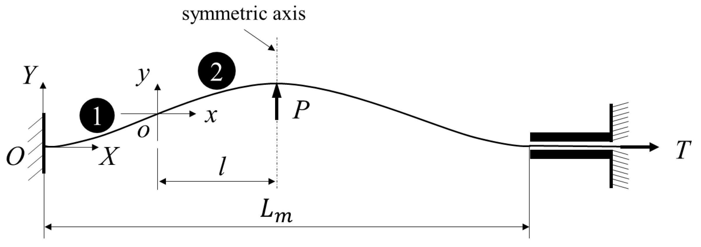
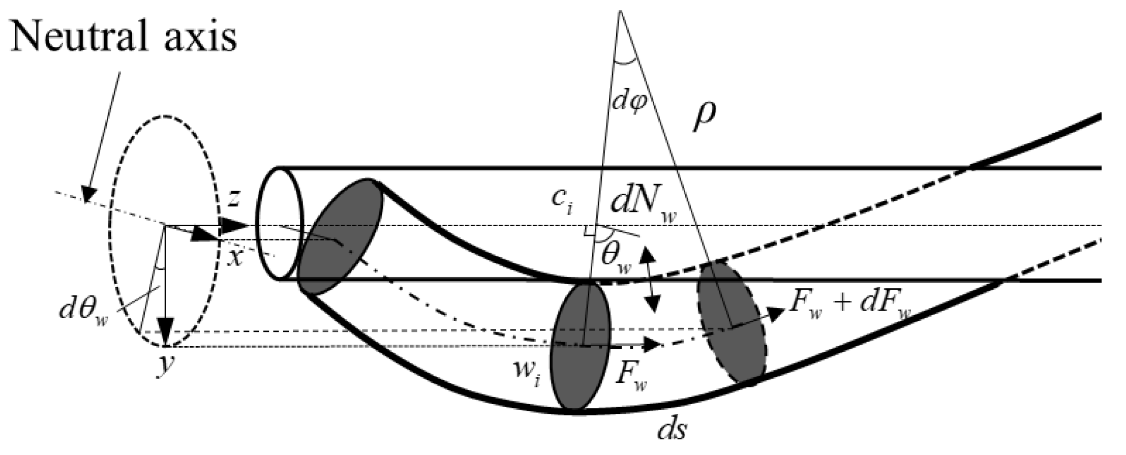
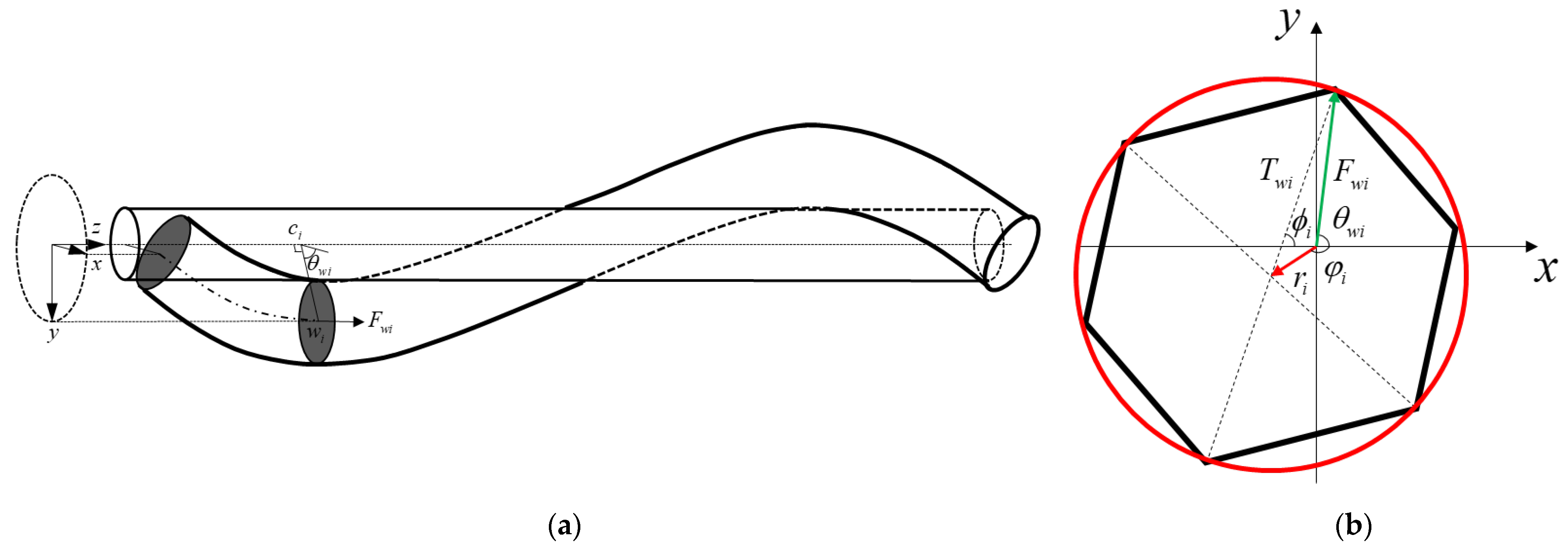
2.2. Approximation of the Deflection of the Simple Strand under Multi-Axial Loadings

A proper fitting function is in the first place proposed to approximate the deflection of the simple strand. It is essential to find out a suitable function that can match the deflection curves. A reasonable idea is that this function is analogical to the deflection formula relative to the linear bending stiffness. The deflection curve expression corresponding to the linear bending stiffness is, therefore, derived in terms of the free bending of the smooth simple strand under multi-axial loadings. Figure 7 illustrates the schematic of free bending. For simplification, only in-plane deformation is considered here. The bending moment is proportional to the curvature for strands with linear bending stiffness, the expression is, therefore, given:

$$M=EI·\kappa$$

(12)

where $M$ denotes the bending moment on the cross-section, $EI$ denotes the linear bending stiffness, and $\kappa$ denotes the in-plane curvature of the strand.

Figure 7 shows the strand bends from a straight line to an arcuate one under the axial tensile force T and the lateral force P whose position is localized on the mid-span. The left end of the strand is constrained with all degrees of freedom, called the fixed-end, and the other end is only released x-translation degree of freedom, called the loading-end. Apparently, the deflection of the whole strand is axially symmetric about the vertical line passing through the lateral loading points. The following work, therefore, focuses on the left part of the whole strand. Additionally, the deflection curve of the left part as marked by ① and ② is centrosymmetric. A cartesian coordinate system xoy is established with the origin coinciding with the mid-point of the left span and the x-axis parallel with the direction of T. Another cartesian coordinate system XOY is fixed at the left end of the strand and its axis is parallel with xoy. The span of the deformed strand is $L_m$, and the horizontal distance between the lateral loading point and the origin o is $l$, whose value is a quarter of the total span.

In the system xoy, the differential equation that defines the deflection for the beam-like strand under the free bending is given by:

$$EI·y^{″}=Ty-\frac{P}{2}x$$

(13)

where $y^{″}$ represents the curvature $\kappa$ because these two are very close in value due to the small deformation assumption.

The general analytical solution of Equation (13) is

$$y=c_1\cosh \left(\lambda x\right)+c_2\sinh \left(\lambda x\right)+\frac{\zeta }{2}x$$

(14)

where $\lambda =\sqrt{\frac{T}{EI}}$, $\zeta$ denotes loading factor and $\zeta =\frac{P}{T}$. The two unknown constants $c_1$ and $c_2$ are determined by the boundary conditions, which are $y\left(0\right)=0$ and $y^{\prime }\left(l\right)=0$,

$$\{\begin{array}{c}{c}_1=0\\ c_2=-\frac{\zeta }{2\lambda }\cosh \left(\lambda l\right)\end{array}$$

(15)

Therefore, the expression of the deflection is:

$$y=-\frac{\zeta }{2\lambda }\frac{\sin \mathrm{h}\left(\lambda x\right)}{\cosh \left(\lambda l\right)}+\frac{\zeta }{2}x$$

(16)

If the original reference frame is replaced with another coordinate system XOY, there exists the following transformation rule:

$$\{\begin{array}{c}x=X-l\\ y=Y+y\left(-l\right)\end{array}$$

(17)

Substituting Equation (17) into Equation (16), the expression of the deflection in the coordinate system XOY is:

$$Y=-\frac{\zeta \left(1-\tan \mathrm{h}\left({\lambda }_l\right)\right)}{4\lambda }{e}^{\lambda X}+\frac{\zeta \left(1+\tan \mathrm{h}\left({\lambda }_l\right)\right)}{4\lambda }{e}^{-\lambda X}+\frac{\zeta }{2}X-\frac{\zeta \tan \mathrm{h}\left({\lambda }_l\right)}{2\lambda }$$

(18)

where ${\lambda }_l$ represents the flexibility factor associated with bending stiffness and ${\lambda }_l=\sqrt{\frac{T{l}^2}{EI}}$.

The value of $\tan \mathrm{h}\left({\lambda }_l\right)$ approaches to 1 when ${\lambda }_l$ is large enough to correspond to the case’s strong tension and long length. Hence, Equation (18) can be simplified as:

$$Y=\frac{\zeta }{2\lambda }\left(e^{-\lambda X}-1\right)+\frac{\zeta }{2}X$$

(19)

Rewriting the above equation in the non-dimensional form, yields:

$$\overline{Y}=\frac{\zeta }{2{\lambda }_p}\left(e^{-{\lambda }_p\overline{X}}-1\right)+\frac{\zeta }{2}\overline{X}$$

(20)

where the overline of the symbol represents the ratio of dimensional quantity and the pitch length, and ${\lambda }_p=\sqrt{\frac{T{p}^2}{EI}}$. It can be seen that the equation of deflection for linear bending stiffness contains an exponential decay term and a linear term. The exponential term is related to bending stiffness and loadings, and the other term is related to loadings only. To determine the expression for the deflection curve of a rope with nonlinear bending stiffness under free bending, the general deflection expression is obtained by replacing the coefficients of the previous equation with coefficients to be determined.

$$\overline{Y}={\chi }_1\left(e^{-{\gamma }_d\overline{X}}-1\right)+{\chi }_2\overline{X}$$

(21)

where ${\gamma }_d={\chi }_1/{\chi }_2$ because the above expression needs to be satisfied with the boundary condition, and ${\chi }_1$, ${\chi }_2$ are unknown coefficients to be determined by fitting a series of scattered data $\left({\overline{x}}_i,{\overline{y}}_i\right)$ on the deflection curve from simulation results by means of the least square method,

$$\left({\chi }_{1,}{\chi }_2\right)=\arg \min {\displaystyle \sum }_{i=1}^n\left|\overline{Y}\left({\overline{x}}_i\right)-{\overline{y}}_i\right|$$

(22)

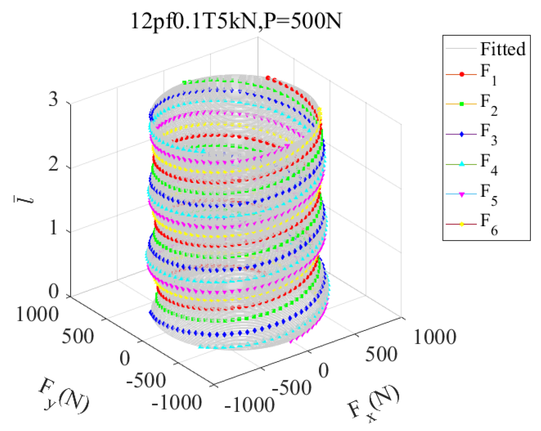
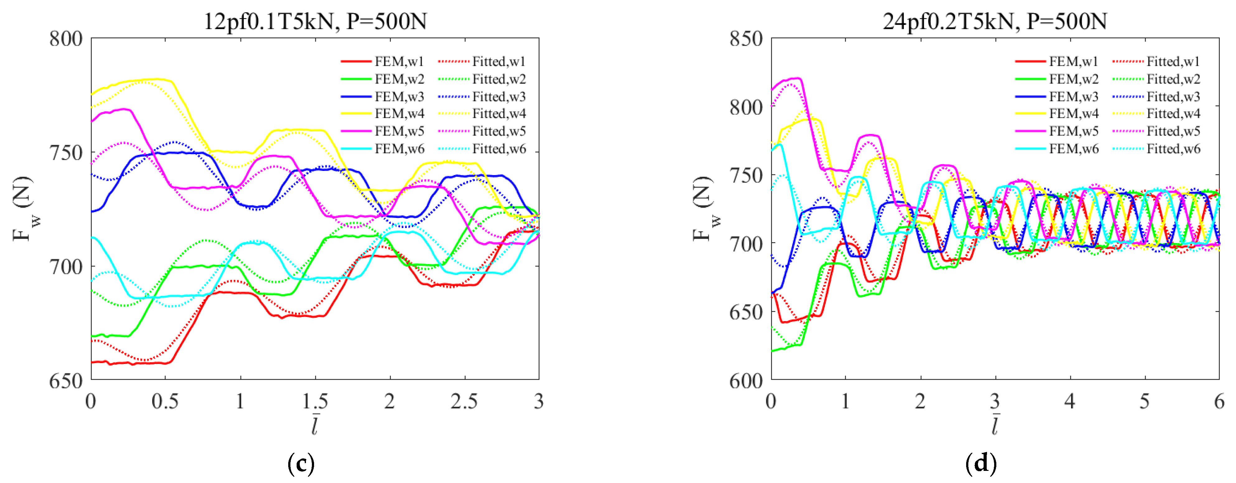
2.3. Approximation of Tension for Individual Wire of the Simple Strand under Multi-Axial Loadings

This section has focused on the evaluation of the tension of each wire based on the simulation results. As for a strand loaded with combinations of axial and lateral loads, the tension of each wire can be obtained by the linear superposition of two parts. One part is contributed by axial tension T, and the other is caused by internal friction.

$$F_{wi}=T_{wi}+f_{wi}$$

(23)

in which $T_{wi}$ is the tensile force acting on the individual wire prior to bending and $f_{wi}$ is the additional tension force induced by friction. $T_{wi}$ can be calculated if the strand is loaded by a tension T.

$$T_{wi}=\frac{A_w{\cos }^2\alpha }{m{A}_w{\cos }^3\alpha +A_c}T$$

(24)

Figure 8a shows a helical wire $w$ wound clockwise around a core wire with a rotation angular. The angular position ${\theta }_{wi}$ is defined as the angle of the line connecting the centers of the core and the wire with respect to the x-axis of the global Cartesian coordinates.

For the node $i$ of wire $w$ in the present FE model, ${\theta }_{wi}$ can be written as:

$${\theta }_{wi}={\theta }_i+{\theta }_{w0}$$

(25)

where ${\theta }_i=\frac{\left(i-1\right)\pi }{36}\overline{l}$ and ${\theta }_{w0}$ denotes the initial angular position of wire $w$.

Assume the relative position of the nodes on each cross-section remains unchanged during the bending, a force group $\left(F_{wi},{\theta }_{wi}\right) | w=1, 2, \dots , 6$ is defined to describe the distributions of tension on the ith cross-section. $F_{wi}$ is axial tension for node i of wire w. The force group on the ith cross-section is drawn in Figure 8b. A force cycle is subsequently defined as $T_{wi}, r_i, {\phi }_i$ to fit the force group on each cross-section of the strand.

$$\left(T_{wi},r_i,{\phi }_i\right)=\arg \min {\displaystyle \sum }_{w=1}^6{T}_{wi}{}^2-{(F_{wi}\cos {\theta }_{wi}-r_i\cos {\phi }_i)}^2-{(F_{wi}\sin {\theta }_{wi}-r_i\sin {\phi }_i)}^2,{\phi }_i\in \left[-\pi ,\pi \right]$$

(26)

$r_i$ is the distance between the center and the coordinate origin, and ${\phi }_i$ is the angular position of the force center with reference to the x-axis which is limited in $\left[-\pi ,\pi \right]$.

Once a sequence of parallel force circles along the strand axis is determined, the magnitude of tension force for each node with angular position ${\theta }_{wi}$ is computed as follows,

$${\widehat{F}}_{wi}=\sqrt{T_{wi}^2+r_i^2+2T_{wi}{r}_i\cos ({\varphi }_i-{\phi }_i)}$$

(27)

where ${\varphi }_i={\theta }_{wi}+\arcsin (\frac{r_i}{T_{wi}}\sin ({\theta }_{wi}-{\phi }_i))$.

The center of each force cycle is denoted as $r_{ix},r_{iy}$. Here, $r_{ix}=r_i\cos {\phi }_i,r_{iy}=r_i\sin {\phi }_i$. These centers form an analogous Archimedean spiral curve in 3-D space, which is induced by uneven tension distribution of outer layer wires around the core. This curve is found to be further fitted by the following equation set by a series of trial and error.

$$\{\begin{array}{l}{r}_{ix}=C_1{e}^{-C_3{\theta }_i}\cos {\theta }_i+C_2{e}^{-C_3{\theta }_i}\sin {\theta }_i+C_4\\ r_{iy}=-C_2{e}^{-C_3{\theta }_i}\cos {\theta }_i+C_1{e}^{-C_3{\theta }_i}\sin {\theta }_i\end{array}.$$

(28)

These unknown coefficients $C_i \left(i=1, 2, 3, 4\right)$ are solved by fitting the $r_i$ curve from force cycles of simulation results. They depend on friction coefficient $\mu$, axial loading factor T and lateral loading factor $\zeta$. There are in total 480 sets of sample data consisting of six levels in friction coefficient and eight levels in axial tension as well as 10 levels in lateral loading. A RSM (response surface methodology) is adopted to establish the relationship between $C_i$ and the above three factors and a linear fitted model is designed,

$$X_i={[x y z xy yz xz x^{2}y x^{2}z x{y}^2 y^{2}z x{z}^2 y{z}^2 xyz]}_i$$

(29)

where $x=\mu$, $y={\lambda }_p$ and $z=\sqrt{\zeta }$.

The response function is $\mathit{Y}=\mathit{X}\mathit{c}$, where $\mathit{Y}={[Y_1,Y_2,\dots ,Y_N]}^T$, $\mathit{X}=\left[X_1;X_2;\dots ;X_N\right]$ and $\mathit{c}={[c_1,c_2,\dots ,c_N]}^T$. The weight coefficients for terms in $X_i$ are determined by:

$$\widehat{\mathit{c}}=\arg \min {\left|\mathit{Y}-{\mathit{C}}_i\right|}^2$$

(30)

to access the goodness of fit, the coefficient of determination, namely R-squared or R² is defined.

$$R^2=1-\frac{{{\displaystyle \sum }}_{i=1}^N{(Y_i-{\widehat{Y}}_i)}^2}{{{\displaystyle \sum }}_{i=1}^N{(Y_i-{\overline{Y}}_i)}^2}$$

(31)

where $Y_i$ is the response data, ${\widehat{Y}}_i$ is the predicted response value, and ${\overline{Y}}_i$ represents the average value of all response values.

Note, that Equation (29) is appropriate for $C_1\sim C_3$, but is cumbersome for $C_4$. By evaluating the effect of each independent variable in $X_i$ on R², the linear fitted model can be simplified to just one term $x{y}^2$ for $C_4$.

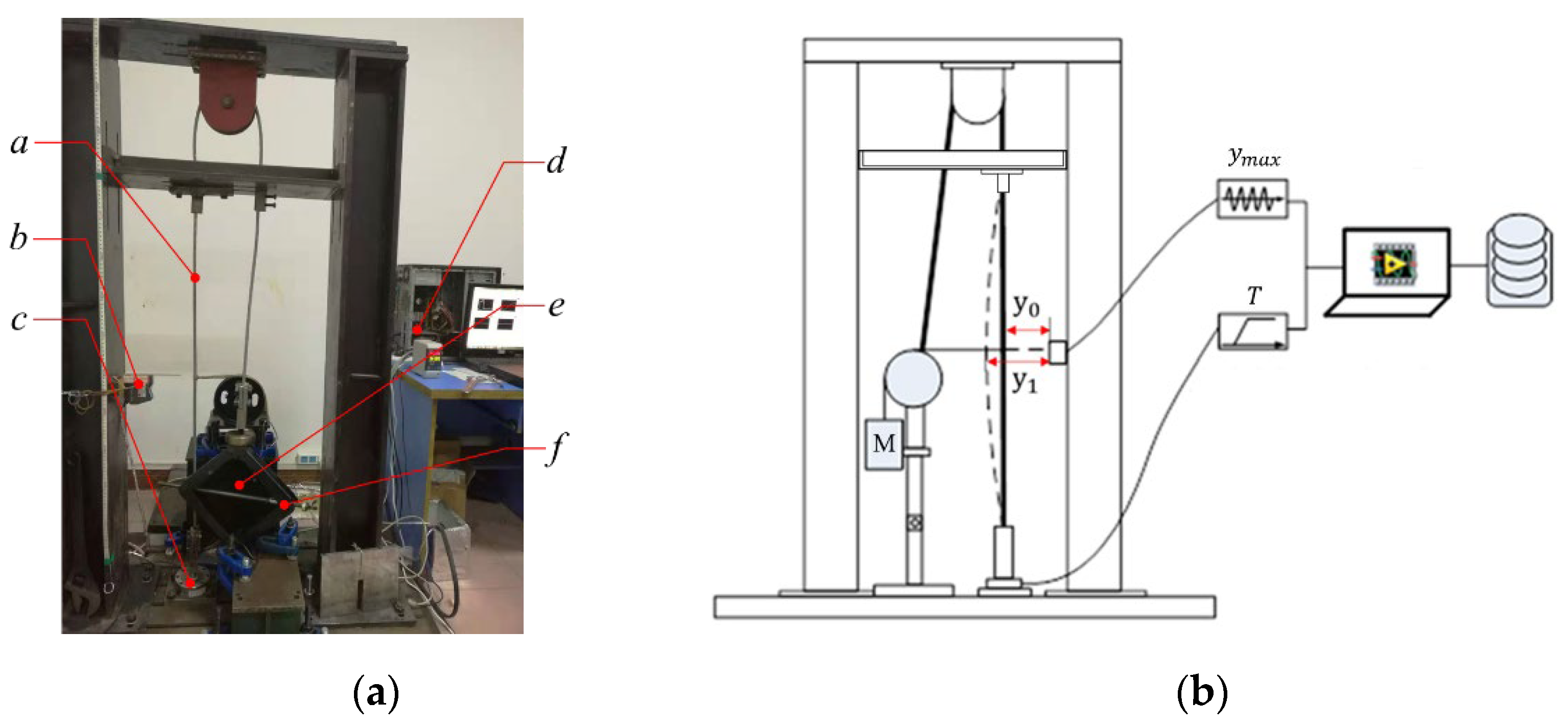
2.4. Experimental Measurement

For further validation of the beam model, a quasi-static free bending experiment was carried out and the associate measurements of maximum deflection at the mid-span of the tested strand under different combinations of axial and lateral loads were recorded to compare with the FE simulation results. A test setup was designed and manufactured to conduct the free bending test for the single-layered strand as presented in Figure 9. In Figure 9a, a represents the tested strand with a length of 0.93 m, nearly seven pitches; b is a laser displacement sensor to measure the deflection of the mid-span of the strand; c is a force transducer to measure the axial tension acting on the strand; d is a data acquisition card to record the electronic signal from the sensors; e is a mass block to apply lateral force on the strand by suspending to the strand, and f is a hand jack to adjust the tension exerted on the strand. One end of the tested strand specimen is fully constrained, and the other end can only move freely in the axial direction.

The deflection of the strand depends on the loading path due to the effect of the nonlinear interwire friction during bending. The displacement will form a hysteretic loop under the action of cyclic lateral force, which means that the similar displacement may correspond to different loadings. Therefore, only a one-way loading method is adopted here.

The description of the experimental measurement is given. Firstly, axial tensile force is applied to the tested strand at a specified value, such as 500 kg, by manually adjusting the jack. Then, the distance, denoted by $y_0$, between the laser displacement sensor and the middle point of the tested strand is recorded as a reference. After that, a mass block is suspended to the middle position of the tested strand and the corresponding measured distance is written down, denoted as $y_1$. At the same time, the real-time tension T subjected to the tested strand should be recorded. Subsequently, turn down the tension of the strand to a new value whose difference with respect to the last value is limited to a range of 25–50 kg. Simultaneously, the values of the deflection and the tension are recorded. Repeat the previous step until the tension reaches the minimum value.

The deflection, $y_{max}$, is the difference between these two recorded distance values, that is $\left|y_1-y_0\right|$, as shown in Figure 9b. The experimental data are listed in

Table 2. Experimental data.

P = 4 kg		P = 8 kg		P = 12 kg		P = 16 kg		P = 20 kg
T/kg	${\mathbf{y}}_{\mathbf{m}\mathbf{a}\mathbf{x}}$/mm	T/kg	${\mathbf{y}}_{\mathbf{m}\mathbf{a}\mathbf{x}}$/mm	T/kg	${\mathbf{y}}_{\mathbf{m}\mathbf{a}\mathbf{x}}$/mm	T/kg	${\mathbf{y}}_{\mathbf{m}\mathbf{a}\mathbf{x}}$/mm	T/kg	${\mathbf{y}}_{\mathbf{m}\mathbf{a}\mathbf{x}}$/mm
102	5.74	100	11.97	101	18.57	99.5	24.79	101	30.57
127	4.79	123	10.21	126	15.33	125	20.64	126	25.70
149	4.18	150	8.62	151	13.10	150.5	17.58	152	22.12
175	3.68	175	7.58	176	11.45	175	15.48	174	19.73
202	3.33	201	6.87	200	10.33	200	13.85	201	17.35
230.8	2.95	221	6.35	225	9.41	225.5	12.59	227	15.70
253	2.65	250	5.64	250	8.53	250.5	11.59	252	14.39
287	2.30	275.5	5.14	272	7.92	275	10.64	278	13.21
304	2.16	299	4.70	300	7.25	298	9.92	301	12.38
331	1.96	325	4.31	326	6.70	325	9.17	326.5	11.46
352	1.83	349	4.00	350	6.23	350	8.55	351	10.70
381	1.67	365	3.83	376	5.77	375	7.92	377	9.99
402.5	1.58	399	3.48	401	5.38	399	7.38	402	9.36
426	1.51	424.5	3.27	425.5	5.09	424	6.90	427	8.76
454	1.44	450	3.11	450	4.85	450.5	6.51	452	8.22
484	1.40	474.5	2.98	475	4.64	475	6.21	477	7.80
528	1.34	499	2.87	500	4.44	500	5.96	502	7.43

. The transverse loads range from 4 kg to 20 kg with an increment of 4 kg. The axial loads are limited in range from 100 kg to 530 kg.

3. Results and Discussion

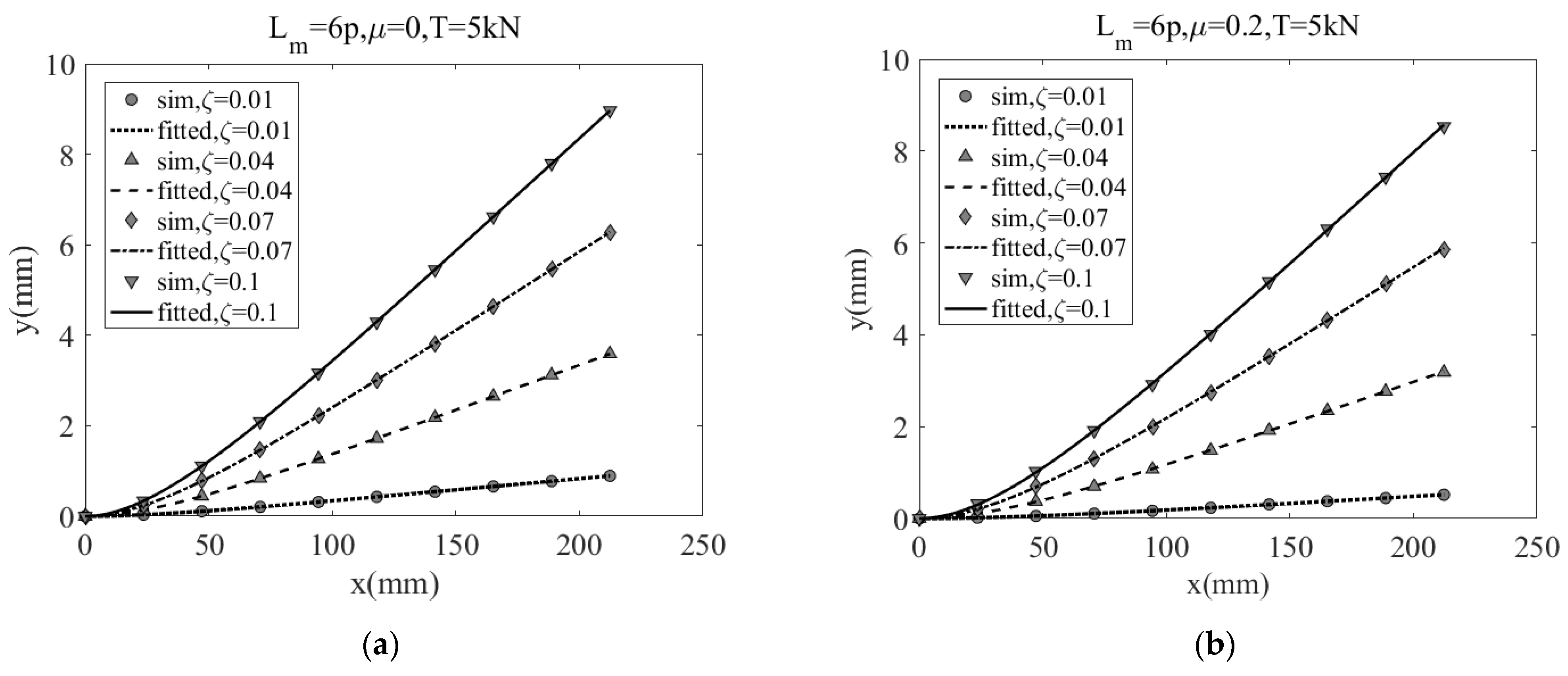
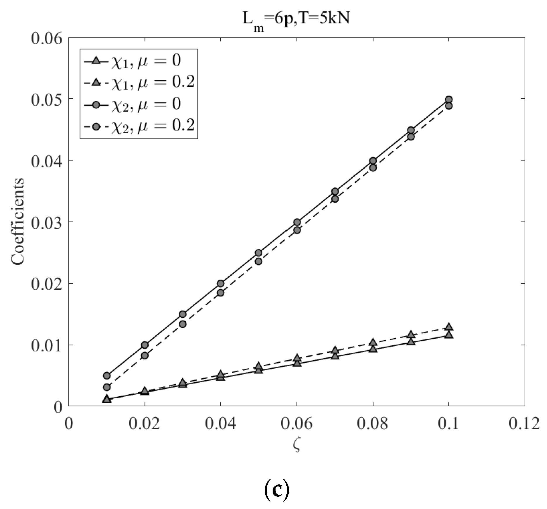
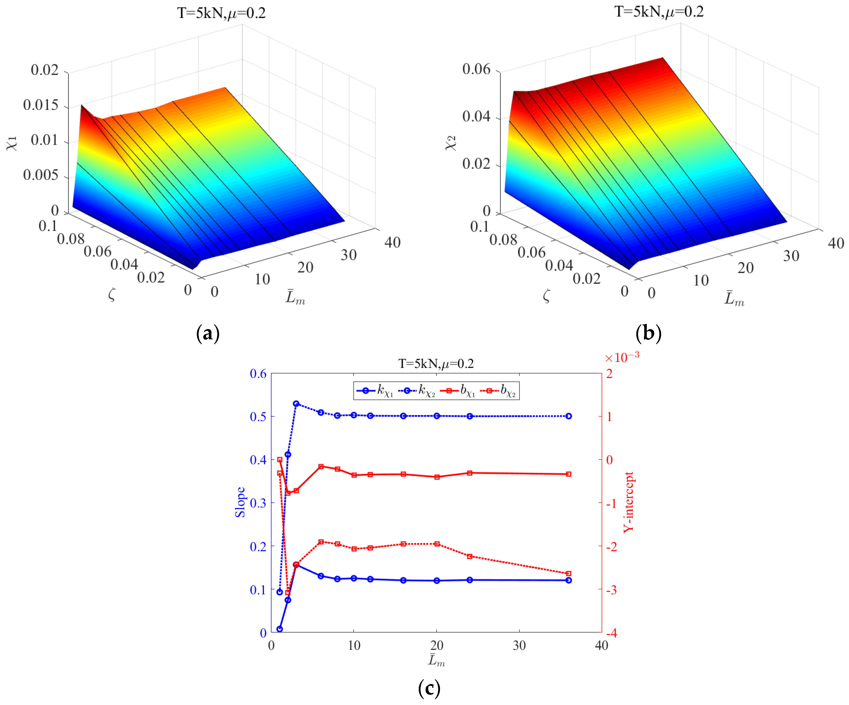
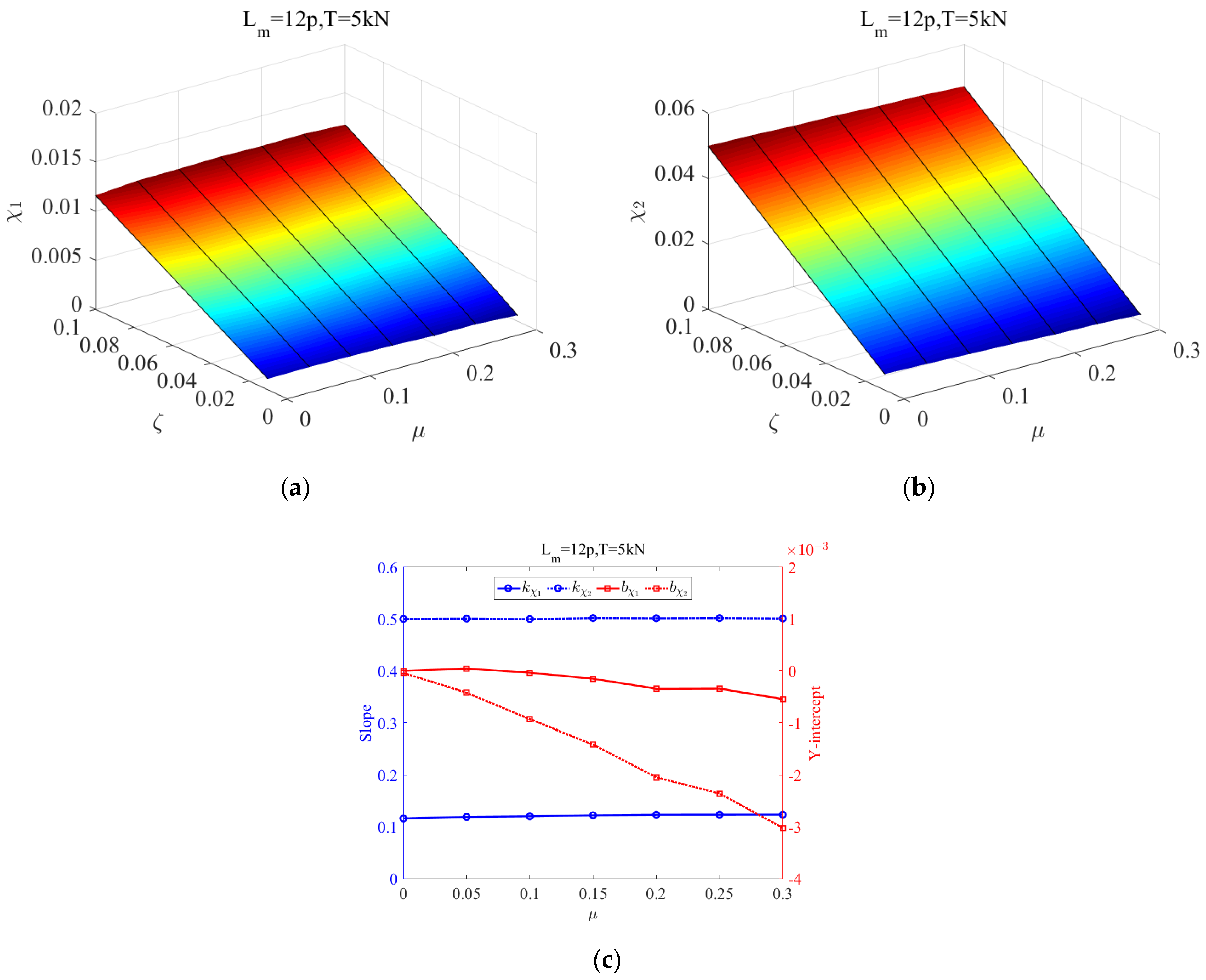
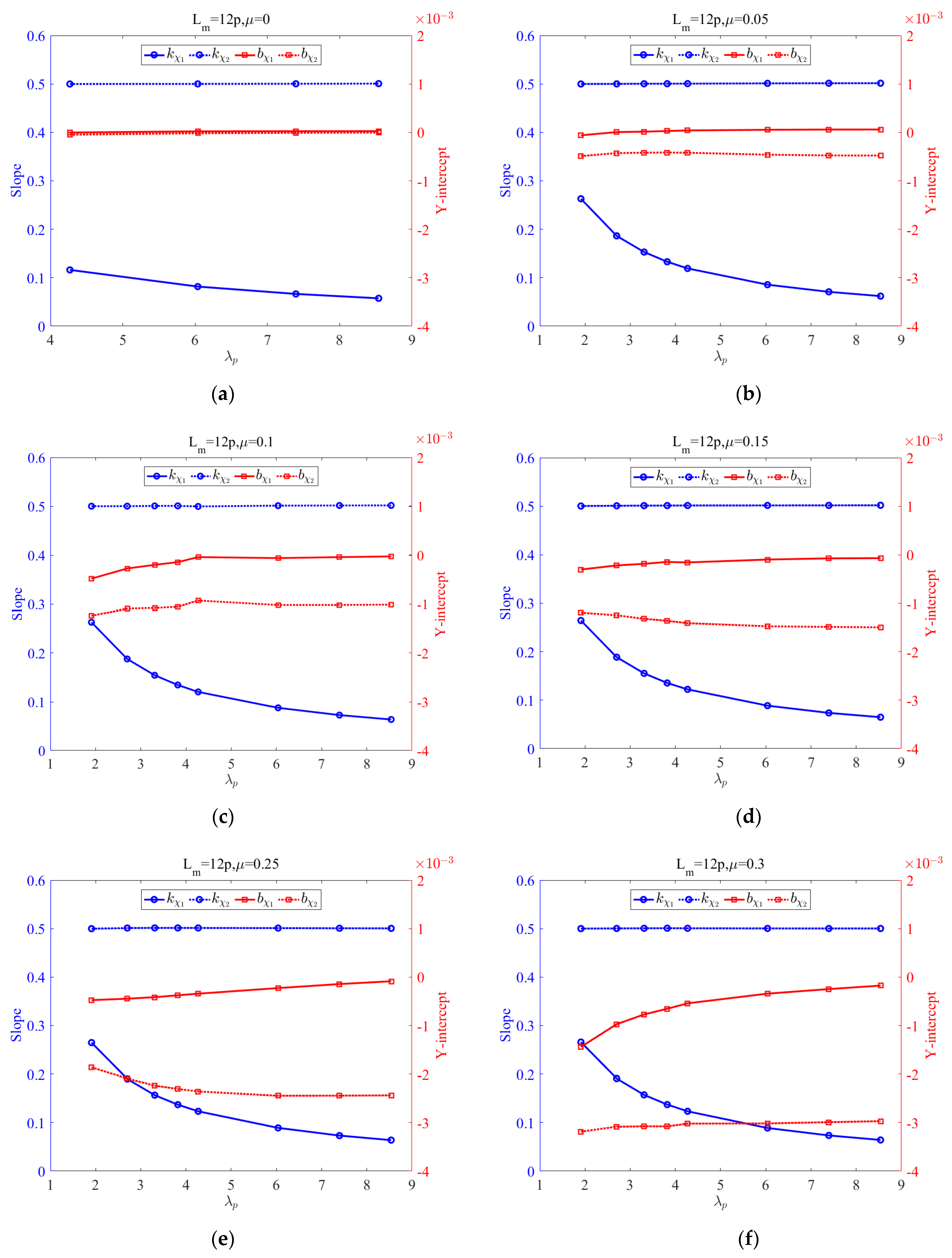
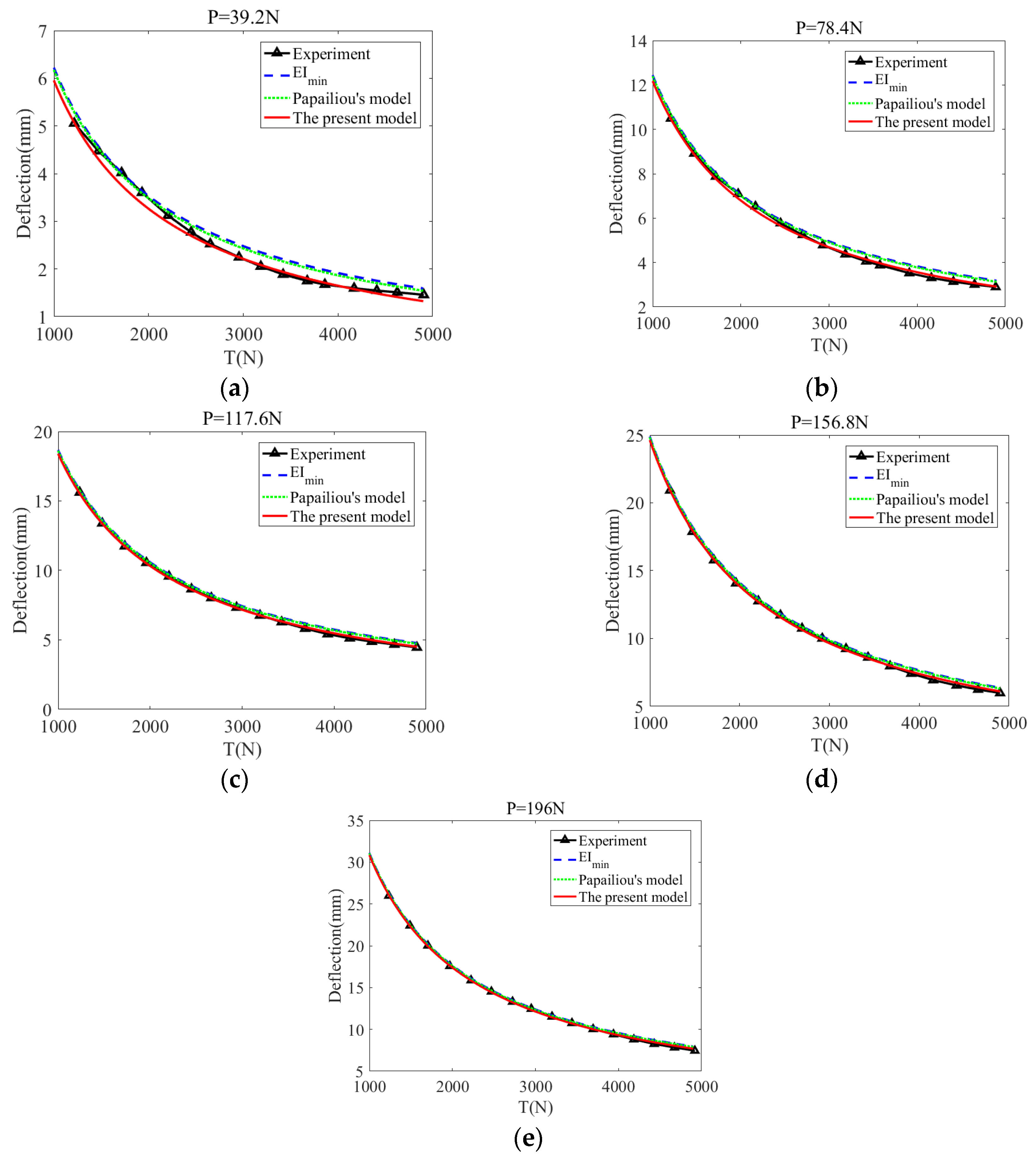
3.1. Effects of Length, Friction and Tension on the Deflection for Simple Strands

Given a loading condition that the axial tension T = 5 kN and lateral force P increasing from 0 to 500 N with an increment of 100 N, two simulations were conducted for two 6-pitch-long strands with different friction coefficients of 0 and 0.2, respectively. A comparison of simulation deflection curves to fitted curves over a quarter of the whole length for four cases in which loading factors $\zeta =0.01, 0.04, 0.07 \mathrm{and} 0.1$, respectively, see Figure 10a,b. It shows that the fitting curves agree well with the simulation results for both strands.

Figure 10c presents the fitting coefficients of the deflection curve under the different loading conditions for strands without friction and with friction coefficient μ = 0.2, respectively. Obviously, it can be seen that there is a linear relationship between the coefficients and the loading factor ζ, no matter whether the strand is smooth or not. Therefore, the coefficients of the fitting function for the deflection curve can be further expressed with respect to ζ.

$${\chi }_i=k_{{\chi }_i}\zeta +b_{{\chi }_i},i=1,2$$

(32)

where $k_{{\chi }_i}$ and $b_{{\chi }_i}$ denote the slope and intercept of the ${\chi }_i-\zeta$ lines, respectively. Similarly, the coefficients can be solved by linear fitting the ${\chi }_i-\zeta$ lines.

The effects of several factors on the bending deformation of the strand are studied. These factors are strand length, friction coefficient, axial tension and lateral force. Nominal strand length ${\overline{L}}_m$ ranges from 1 to 36, frictional coefficient changes from 0 to 0.3 with an increment of 0.05, and axial tension increases from 1 kN to 20 kN. The nominal lateral loading factor $\zeta$ varies from 0.01 to 0.1.

Table 3. Factors and levels for parametric analysis.

Factors	Levels
Nominal length ${\overline{\mathit{L}}}_{\mathit{m}}$	1, 2, 3, 6, 8, 10, 12, 16, 24, 36
Friction coefficients μ	0, 0.05, 0.1, 0.15, 0.2, 0.25, 0.3
Axial tension T (kN)	1, 2, 3, 4, 5, 10, 15, 20
Nominal lateral loading factor ζ	0.01, 0.02, 0.03, 0.04, 0.05, 0.06, 0.07, 0.08, 0.09, 0.1

lists the factors and levels for the parametric analysis on the effect of lateral deformation of spiral strands under free bending.

Figure 11a,b illustrates 3D plots of the fitting coefficients ${\chi }_1$ and ${\chi }_2$ of the general deflection curve equation for strands with different lengths at a constant axial tension of 5 kN and varying lateral loadings, respectively. These two coefficients are sensitive to strand length in cases ${\overline{L}}_m<3$, but the lines gradually tend to stabilize after the strand length exceeds six pitches. It indicates the effects of boundary condition on deflection gradually declines as the length increases. Figure 11c presents the slope and intercept defined in Equation (32) for each strand with a specified length. It is found that both the slope and intercept of the fitting coefficients of the deflection curve almost keep constant as the strand length exceeds 6 pitches.

Figure 12a,b displays 3D plots of ${\chi }_1$ and ${\chi }_2$ for strands with different friction coefficients ranging from 0 to 0.3. The nominal strand length is specified as 12 pitches, as mentioned before, this strand length has little effect on the ${\chi }_i$. The axial tension is set to 5 kN. From the figures, it can be seen that these three variables, which are ${\chi }_i$, $\zeta$ and $\mu$, show a linear relationship with each other. The slope and intercept of the fitting coefficients are further obtained from the 3D plot, see Figure 12c. The parameter $b_{{\chi }_2}$ of the coefficient array, changes most significantly with an increased friction coefficient as a slight variation as $\mu$ increases. The other two coefficients hardly vary with $\mu$.

Finally, the effect of axial tension on the coefficient array is analyzed. The 3D plot of ${\chi }_1-\zeta -{\lambda }_p$ exhibits a concave surface, but that of ${\chi }_2-\zeta -{\lambda }_p$ appears a flat plane (as shown in Figure 13a,b). Figure 13c gives a plot of the variation of the coefficient array with nominal axial tension ${\lambda }_p$. The slope of the fitting coefficient ${\chi }_1$ with respect to $\zeta$, namely $k_{{\chi }_1}$, has a distinct downward tendency with the increasing of ${\lambda }_p$.

In fact, it is possible that there exists a couple of effects of tension and friction on the slope and intercepts due to the friction inside the strand being affected by these two factors. There is, therefore, a need to observe regularities for strands with different friction coefficients at different levels of tension force except for those discussed above; the results are presented in Figure 14a–f.

For strands with different friction coefficients, the variation trend of the first two slopes with nominal tensile force remains almost unchanged, while the other two coefficients change greatly, especially for the last one. The last two coefficients keep constant and $b_{{\chi }_1}$ approaches to 0 in cases where ${\lambda }_p\ge 4$ and $\mu \le 2,$ in particular. Moreover, it can be inferred from Figure 12c that $b_{{\chi }_2}$ is proportional to $\mu$. Consequently, the generalized fitting equation given in Equation (19) can be further simplified in the following form:

$$\overline{Y}=\frac{\zeta }{2}(\frac{e^{-{\lambda }_p\overline{X}}-1}{{\lambda }_p}+\overline{X})-k_{\mu }\mu \overline{X}$$

(33)

where $k_{\mu }$ is the proportionality factor of $b_{{\chi }_2}$ with respect to $\mu$.

For the present simple strand, the proportionality factor $k_{\mu }$ = 0.01 and the friction coefficient μ = 0.115.

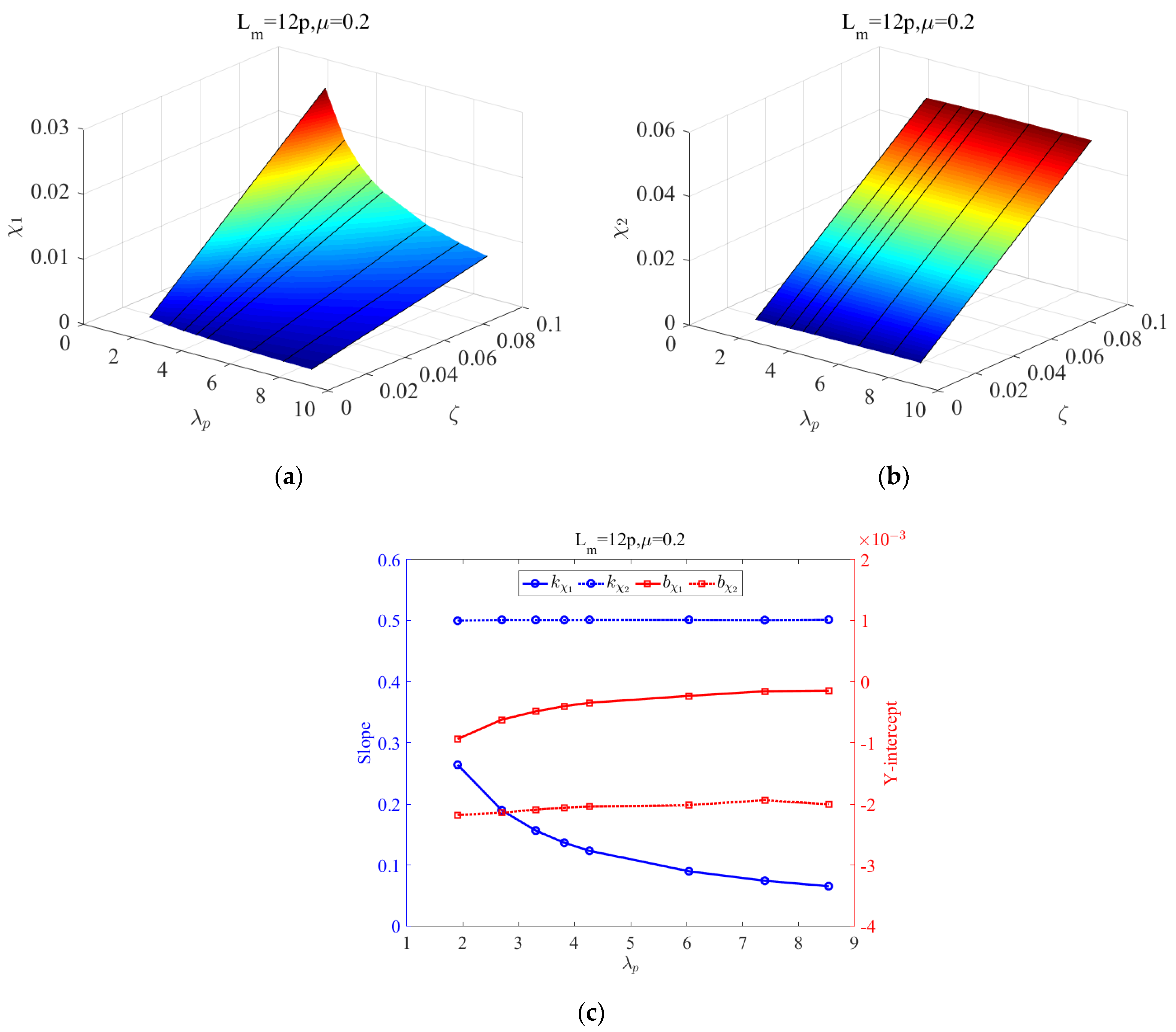
3.2. An Analytical Model from Papailiou’s Theory and Comparision Analysis

For the purpose of comparison, an analytical model is derived from Papailiou’s theory. Taking an infinitesimal segment ds on an arbitrary wire as a research object, as shown in Figure 15, the slippage criterion governing the tension distribution for each wire is expressed as follows:

$$\left|d{F}_w\right|\le \mu d{N}_w,$$

(34)

where $F_w$ is the tension of the wire and $d{N}_w$ is the normal contact force on an infinitesimal segment.

Based on the principles of force balance, there exists a relation between the tension and the normal contact force.

$$d{N}_w=F_{w}d\phi$$

(35)

According to the geometric relation, the length of the infinitesimal segment is calculated:

$$ds=\rho d\phi =\frac{R_{h}d{\theta }_w}{\sin \alpha }$$

(36)

where $\rho$ represents the radius of the curvature of the outside wire and ${\theta }_w$ represents the included angle between the neutral axis and the vector point from the centroid of the strand to the centroid of the wire w (w takes a value from 1 to 6 here) on a specified cross-section as shown in Figure 15.

Assuming that the bending deformation is small, the radius of the curvature of the current deformed wire is identical to its initial value ${\kappa }_0$. Thus,

$$\rho =\frac{1}{{\kappa }_0}=\frac{R_h}{{\sin }^2\alpha }$$

(37)

Substituting Equations (35)–(37) into Equation (34), the slippage criterion is rewritten as:

$$\left|d{F}_w\right|\le \mu F_w\sin \alpha d{\theta }_w$$

(38)

The angular position of the centroid of the wire ${\theta }_w$ locates in the range $\left[-\frac{\pi }{2},\frac{\pi }{2}\right]$. The axial tension is assumed to increase with the increasing angular position, and thus $d{F}_w>0$.

For the slip region, the solution of the differential Equation (38) is:

$$F_{w,slip}=T_0{e}^{\mu {\theta }_w\sin \alpha }$$

(39)

where $T_0$ is the tension at the angular position ${\theta }_w=0$.

$$T_0=E{A}_w{\epsilon }_c{\cos }^2\alpha$$

(40)

The axial strain ${\epsilon }_c$ of the strand and depends on the total tensile force of the strand $T$ as approximated by:

$${\epsilon }_c=\frac{T}{E{A}_c+6E{A}_w{\cos }^3\alpha }$$

(41)

Before the inside slippage happens, the tension of the individual wire satisfies:

$$F_{w,stick}=E{A}_w{\cos }^2\alpha \left({\epsilon }_c+R_h\kappa \sin {\theta }_w\right)$$

(42)

With the curvature of the strand increasing from 0 to a certain value, the contact state between adjacent wires changes from the original stick state to a slip state. Assuming the critical curvature is ${\kappa }_c$, the maximum slip tension is equal to the static tension at the critical position:

$$E{A}_w{\epsilon }_c{\cos }^2\alpha ·e^{\mu {\theta }_w\sin \alpha }=E{A}_w{\cos }^2\alpha \left({\epsilon }_c+R_h\kappa \sin {\theta }_w\right)$$

(43)

Therefore, the critical curvature can be solved as given below:

$${\kappa }_c=\frac{\left(e^{\mu {\theta }_w\sin \alpha }-1\right){\epsilon }_c}{R_h\sin {\theta }_w}.$$

(44)

The axial tension for each wire on a specified cross-section can thus be given as follows:

$$F_w\left({\theta }_w\right)=\{\begin{array}{c}min({\epsilon }_c{e}^{\mu {\theta }_w\sin \alpha },R_h\kappa \sin {\theta }_w+{\epsilon }_c)\cdot E{A}_w{\cos }^2\alpha ,{\theta }_w\ge 0\\ max({\epsilon }_c{e}^{\mu {\theta }_w\sin \alpha },R_h\kappa \sin {\theta }_w+{\epsilon }_c)\cdot E{A}_w{\cos }^2\alpha ,{\theta }_w<0\end{array}$$

(45)

For ease of presentation, the outside wires of the strand are anticlockwise numbered as presented in Figure 16, the angular position for each wire depends on an initial angular position ${\theta }_0$ as given by:

$$\mathit{\Phi }=\left[{\theta }_1,{\theta }_2,\cdots ,{\theta }_6\right]=\left[{\theta }_0,\frac{\pi }{2}-\left|{\theta }_0-\frac{\pi }{6}\right|,\frac{\pi }{3}-{\theta }_0,-{\theta }_0,\left|{\theta }_0-\frac{\pi }{6}\right|-\frac{\pi }{2},{\theta }_0-\frac{\pi }{3}\right]$$

(46)

and $0\le {\theta }_0<\frac{\pi }{3}$.

Consequently, the whole bending moment of the strand with respect to the curvature could be obtained by superposing the bending moment generated by each wire referring to the neutral axis of the strand.

$$M=\left(6E{I}_w\cos \alpha +E{I}_c\right)\kappa +{\displaystyle \sum }_{i=1}^{6}T\left({\theta }_w\right)R_h\sin {\theta }_w\cos \alpha$$

(47)

where M is the bending moment on a specified cross-section of the strand, $E{I}_w$ denotes the bending stiffness of the outside wire, $E{I}_c$ denotes the bending stiffness of the core wire.

The bending moment M can be assumed to be a function with respect to the curvature κ as given by:

$$M=f\left(\kappa \right)$$

(48)

Assuming that the continuous strand is divided into N-1 segments, an orthogonal coordinate system oxy is defined as shown in Figure 17. Note, that the origin of the coordinate is located at the point where the bending moment is equal to zero. The deflection for the deformed strand is expressed as $\mathit{y}={\left\{y_1,y_2,\cdots ,y_N\right\}}^T$ and then, the bending moment $M_i$ at $x_i$ is given by:

$$M_i=T{y}_i-0.5P{x}_i$$

(49)

Only the small deformation is considered here, the corresponding curvature ${\kappa }_i$ is, therefore, approximated by the central difference method:

$${\kappa }_i=\frac{y_{i-1}+y_{i+1}-2y_i}{h^2}$$

(50)

where $h=\frac{L_m}{N-1}$.

Since both two ends of the strand are clamped, the boundary conditions are:

$$y^{\prime }\left(x_1\right)=y^{\prime }\left(x_N\right)=0$$

(51)

An N-dimensional set of equations $\mathit{F}\left(\mathit{y}\right)$ with respect to $\mathit{y}$ is obtained,

$$F_i=\{\begin{array}{c}1.5y_1-2y_2+0.5y_3,i=1;\\ \begin{array}{c}{y}_{i-1}+y_{i+1}-2y_i-h^2{f}^{-1}\left(M_i\right),i=2~N-1;\\ 1.5y_N-2y_{N-1}+0.5y_{N-2},i=N.\end{array}\end{array}$$

(52)

The true deflection ${\mathit{y}}^{*}$ is satisfied with the following expression:

$$\mathit{F}\left({\mathit{y}}^{*}\right)=\mathbf{0}$$

(53)

Newton’s iteration method is applied to solve the above equations, the criterion is expressed as follows and the iteration termination condition is $\parallel {\mathit{y}}^{\left(\mathrm{k}+1\right)}-{\mathit{y}}^{\left(k\right)}\parallel \le 1\times {10}^{-6}$.

$$\{\begin{array}{c}{\mathit{y}}^{\left(\mathrm{k}+1\right)}={\mathit{y}}^{\left(k\right)}-{\mathit{G}}^{-1}\left({\mathit{y}}^{\left(k\right)}\right)\mathit{F}\left({\mathit{y}}^{\left(k\right)}\right)\\ {\mathit{y}}^{\left(0\right)}={\mathit{y}}_0\end{array}$$

(54)

where $\mathit{G}$ is the Jacobian Matrix and its component $G_{ij}=\frac{\partial F_i}{\partial y_j}$, ${\mathit{y}}_0$ is the deflection corresponding to the minimum bending stiffness $E{I}_{min}$, and $k$ denotes the k-th iteration.

Figure 18 compares the predicted values to analytical values associated with minimum bending stiffness and theoretical values obtained from Papailiou’s model as well as the experimental measurements. The results demonstrate that the proposed model is quite satisfactory to estimate the bending deflections for frictional simple strands subjected to multi-axial loads. Figure 19 presents the relative error between the results from the present model and the experimental measurements. It can be seen that the maximum error is less than 10%.

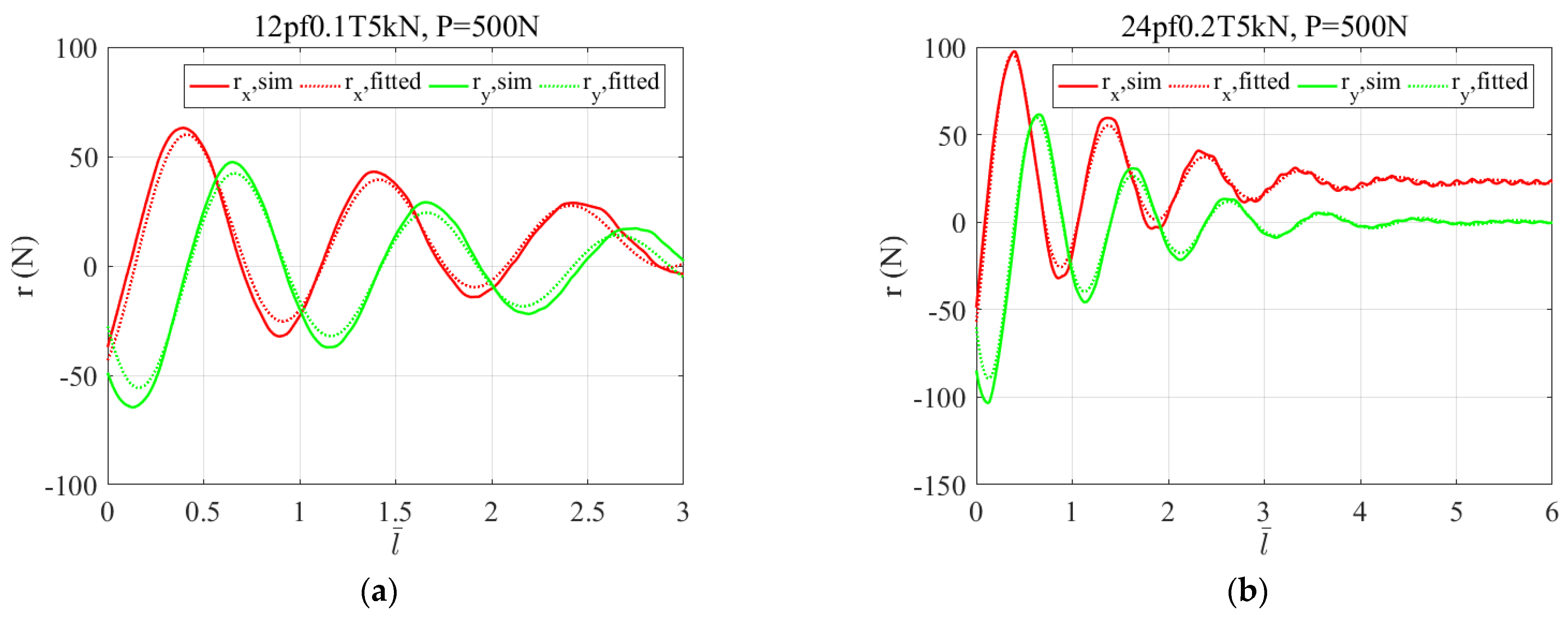
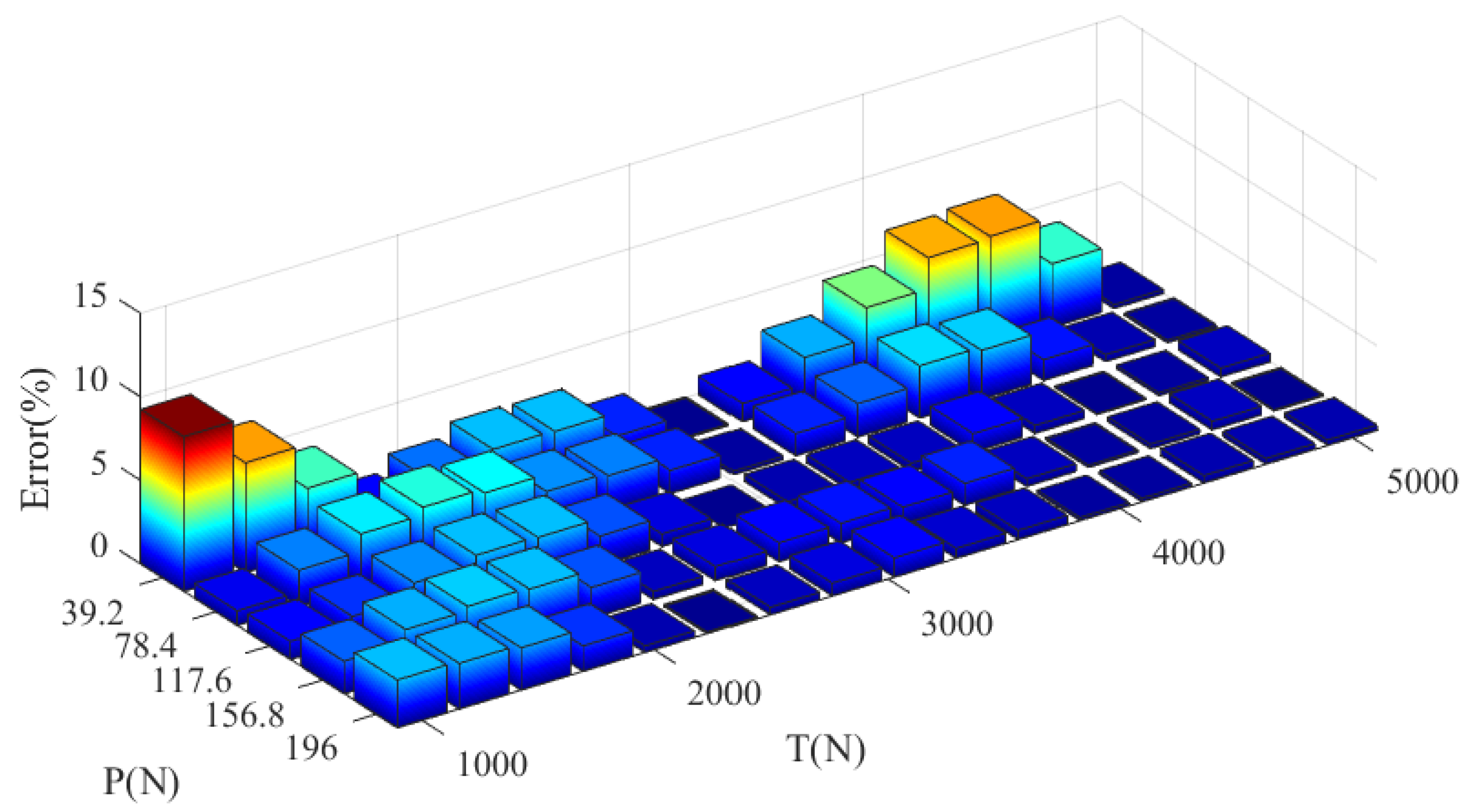
3.3. Tension Estimation for Frictional Strand under Different Loads

Table 4. $c_i$ coefficients and R-squared for 12-pitch-long strand.

${\mathit{c}}_{\mathit{i}}$	C1	C2	C3	C4
c1	29.0682	81.2622	3.9885	--
c2	3.8947	−10.5819	0.0387	--
c3	21.0599	195.6334	0.1034	--
c4	−33.1358	54.2467	0.1468	--
c5	−33.3216	−22.2503	−0.2001	--
c6	−49.1485	−1559.0403	−27.6557	--
c7	143.9697	−328.7151	−0.4003	--
c8	−625.9817	3172.6300	5.4847	--
c9	1.1374	2.9707	−0.0021	6.2839
c10	−2.3024	13.5124	−0.0043	--
c11	1884.4129	−2257.9039	42.2574	--
c12	33.0398	−180.9647	0.3377	--
c13	−341.1416	588.8275	0.2601	--
R2	0.9959	0.9909	0.9847	0.9998

presents the results of fitting coefficients and R² for C₁–C₄, respectively. It can be seen that the values of all R² are very close to 1, which indicates that the goodness of fit is excellent.

Figure 20 exhibits that the force cycles fit well with the simulation results for a 12-pitch-long strand with a friction coefficient of 0.1 and subjected to T = 5 kN and P= 500 N. It demonstrates that it is reasonable to describe the tension distribution along the outer layer wires by a surface consisting of a sequence of parallel force circles.

Figure 21a compares the predicted values of $r_x$ and $r_y$ to that of simulation results for the case where μ = 0.1 and T = 5 kN as well as ζ = 0.1. The results show that the variation regularity of projections of the summation of tension force of outer wires on the global x-axis and y-axis is well predicted. As mentioned before, the weight coefficients of the linear model are determined based on the simulation results from strands with 12-pitch in length. A test example whose length is 24 pitches is simulated to verify the correctness of the fitted model. In this example, the friction coefficient is set to 0.2 and the axial tension is 5 kN. It can be seen from Figure 21b that the fitted numerical model is also suitable for a 24-pitch-long strand. The tension of the outer layer wire along the strand axis can be further obtained by substituting the value of $r$ into Equation (25), as shown in Figure 21c,d. Obviously, the numerical results for the 24-pitch-long strand are closer to simulation results than that for the 12-pitch-long strand. It is, therefore, inferred that the present numerical model is of the ability to estimate the tension of wire for strands with a longer length.

4. Conclusions

This paper proposed a beam FE model to investigate the bending mechanism for a typical single-layered strand subjected to multi-axial loads. A penalty stiffness algorithm incorporating a Coulomb friction model is implemented into the FE model to ensure the precise estimation for interwire friction without any assumptions. It is suitable for strands with more complex geometry and longer length because the present model remarkably reduces the number of beam elements.

The influence of strand length on deflection, seldom mentioned in previous research, is discussed here. It indicated that the influence was diminished with the increase of the length and almost disappeared as the strand length exceeds six times pitch length.

Subsequently, a general deflection expression was extended from a classic Euler beam theory to predict the lateral deformation for frictional strands subjected to multi-axis loads based on the small deformation assumption. This expression fitted well with the simulation results. The resistance of the friction on the bending deformation was clearly characterized. The deflection consists of two terms, one is related to the bending stiffness of individual constituent wire and another term corresponds to the resistance of friction. Moreover, this expression was proved to be quietly accurate since it precisely predicted the sag deflections in accordance with the experimental measurements for a simple strand under free bending. The relative error of the proposed model with respect to experimental measurements is less than 10%.

Furthermore, additional axial tension induced by the interwire friction was apparently presented and the uneven force distribution caused the out-plan deformation of the spiral strand under the in-plan loading. An expression analogous to the parametric equation of Archimedes helix was proposed and utilized to estimate the additional tension for the individual wire in the outer layer of the strand. The coefficient for this expression was determined by means of RSM based on the simulation results. Compared with the FE results, this present method can well predict the tension for individual wires for frictional spiral strands under free bending. It provided an innovative insight for further analytical study to alter the assumptions on the slippage criterion.

References

1. Ni, Y.Q.; Ko, J.M.; Zheng, G. Dynamic analysis of large-diameter sagged cables taking into account flexural rigidity. J. Sound Vib. 2002, 257, 301–319. [Google Scholar] [CrossRef]
2. Levesque, F.; Goudreau, S.; Langlois, S.; Legeron, F. Experimental study of dynamic bending stiffness of ACSR overhead conductors. IEEE Trans. Power Deliv. 2015, 30, 2252–2259. [Google Scholar] [CrossRef] [Green Version]
3. Langlois, S.; Legeron, F.; Levesque, F. Time history modeling of vibrations on overhead conductors with variable bending stiffness. IEEE Trans. Power Deliv. 2014, 29, 607–614. [Google Scholar] [CrossRef]
4. Zhu, Z.H.; Meguid, S.A. Nonlinear FE-based investigation of flexural damping of slacking wire cables. Int. J. Solids Struct. 2007, 44, 5122–5132. [Google Scholar] [CrossRef] [Green Version]
5. Foti, F.; Martinelli, L.; Perotti, F. A new approach to the definition of self-damping for stranded cables. Meccanica 2016, 51, 2827–2845. [Google Scholar] [CrossRef]
6. Dastous, J.B. Nonlinear finite-element analysis of stranded conductors with variable bending stiffness using the tangent stiffness method. IEEE Trans. Power Deliv. 2005, 20, 328–338. [Google Scholar] [CrossRef]
7. McConnell, K.G.; Zemke, W.P. The measurement of flexural stiffness of multistranded electrical conductors while under tension. Exp. Mech. 1980, 20, 198–204. [Google Scholar] [CrossRef]
8. Filiatrault, A.; Christopher, S. Flexural properties of flexible conductors interconnecting electrical substation equipment. J. Struct. Eng. 2005, 131, 151–159. [Google Scholar] [CrossRef]
9. Chen, Z.; Yu, Y.; Wang, X.; Wu, X.; Liu, H. Experimental research on bending performance of structural cable. Constr. Build. Mater. 2015, 96, 279–288. [Google Scholar] [CrossRef]
10. Love, A.E.H. A Treatise on the Mathematical Theory of Elasticity; Cambridge University Press: Cambridge, UK, 2013. [Google Scholar]
11. Costello, G.A. Theory of Wire Rope, 2nd ed.; Springer: New York, NY, USA, 1997. [Google Scholar]
12. Cao, X.; Wu, W.G. The establishment of a mechanics model of multi-strand wire rope subjected to bending load with finite element simulation and experimental verification. Int. J. Mech. Sci. 2018, 142, 289–303. [Google Scholar] [CrossRef]
13. LeClair, R.A.; Costello, G.A. Axial, bending and torsional loading of a strand with friction. J. Offshore Mech. Arct. Eng. 1988, 110, 38–42. [Google Scholar] [CrossRef]
14. Chen, Y.; Meng, F.; Gong, X. Study on performance of bended spiral strand with interwire frictional contact. Int. J. Mech. Sci. 2017, 128, 499–511. [Google Scholar] [CrossRef]
15. Ramsey, H. A theory of thin rods with application to helical constituent wires in cables. Int. J. Mech. Sci. 1988, 30, 559–570. [Google Scholar] [CrossRef]
16. Raoof, M.; Hobbs, R. The bending of spiral strand and armored cables close to terminations. J. Energy Resour. Technol. 1984, 106, 349–355. [Google Scholar] [CrossRef]
17. Jolicoeur, C.; Cardou, A. Semicontinuous mathematical model for bending of multilayered wire strands. J. Eng. Mech. 1996, 122, 643–650. [Google Scholar] [CrossRef]
18. Cardou, A.; Jolicoeur, C. Mechanical models of helical strands. Appl. Mech. Rev. 1997, 50, 1–14. [Google Scholar] [CrossRef]
19. Lanteigne, J. Theoretical estimation of the response of helically armored cables to tension, torsion, and bending. J. Appl. Mech. 1985, 52, 423–432. [Google Scholar] [CrossRef]
20. Papailiou, K.O. On the bending stiffness of transmission line conductors. IEEE Trans. Power Deliv. 1997, 12, 1576–1588. [Google Scholar] [CrossRef]
21. Hobbs, R.E.; Ghavani, K. The fatigue of structural wire strands. Int. J. Fatigue 1982, 4, 69–72. [Google Scholar] [CrossRef]
22. Hong, K.J.; Kiureghian, A.D.; Sackman, J.L. Bending behavior of helically wrapped cables. J. Eng. Mech. 2005, 131, 500–511. [Google Scholar] [CrossRef]
23. Foti, F.; Martinelli, L. Mechanical modeling of metallic strands subjected to tension, torsion and bending. Int. J. Solids Struct. 2016, 91, 1–17. [Google Scholar] [CrossRef]
24. Foti, F.; Martinelli, L. An analytical approach to model the hysteretic bending behavior of spiral strands. Appl. Math. Model. 2016, 40, 6451–6467. [Google Scholar] [CrossRef]
25. Khan, S.W.; Gencturk, B.; Shahzada, K.; Ullah, A. Bending behaviour of axially preloaded multilayered spiral strands. J. Eng. Mech. 2018, 144, 04018112. [Google Scholar] [CrossRef]
26. Zheng, X.; Hu, Y.; Zhou, B.; Li, J. Modelling of the hysteretic bending behavior for helical strands under multi-axial loads. Appl. Math. Model. 2021, 97, 536–558. [Google Scholar] [CrossRef]
27. Nawrocki, A.; Labrosse, M. A finite element model for simple straight wire rope strands. Comput. Struct. 2000, 77, 345–359. [Google Scholar] [CrossRef]
28. Yu, Y.J.; Chen, Z.H.; Liu, H.B.; Wang, X.D. Finite element study of behavior and interface force conditions of seven-wire strand under axial and lateral loading. Constr. Build. Mater. 2014, 66, 10–18. [Google Scholar] [CrossRef]
29. Judge, R.; Yang, Z.; Jones, S.W.; Beattie, G. Full 3D finite element modelling of spiral strand cables. Constr. Build. Mater. 2012, 35, 452–459. [Google Scholar] [CrossRef]
30. Kmet, S.; Stanova, E.; Fedorko, G.; Fabian, M.; Brodniansky, J. Experimental investigation and finite element analysis of a four-layered spiral strand bent over a curved support. Eng. Struct. 2013, 57, 475–483. [Google Scholar] [CrossRef]
31. Xing, E.; Zhou, C. Analysis of the bending behavior of a cable structure under microgravity. Int. J. Mech. Sci. 2016, 114, 132–140. [Google Scholar] [CrossRef]
32. Zhang, D.; Martin, O.S. Finite element solutions to the bending stiffness of a single-layered helically wound cable with internal friction. J. Appl. Mech. 2016, 83, 031003. [Google Scholar] [CrossRef]
33. Jiang, W.G.; Yao, M.S.; Walton, J.M. A concise finite element model for simple straight wire rope strand. Int. J. Mech. Sci. 1999, 41, 143–161. [Google Scholar] [CrossRef]
34. Jiang, W.G.; Henshall, J.L.; Walton, J.M. A concise finite element model for three-layered straight wire rope strand. Int. J. Mech. Sci. 2000, 42, 63–86. [Google Scholar] [CrossRef]
35. Kim, S.-Y.; Lee, P.-S. Modeling of helically stranded cables using multiple beam finite elements and its application to torque balance design. Constr. Build. Mater. 2017, 151, 591–606. [Google Scholar] [CrossRef]
36. Yu, Y.; Wang, X.; Chen, Z. A simplified finite element model for structural cable bending mechanism. Int. J. Mech. Sci. 2016, 113, 196–210. [Google Scholar] [CrossRef]
37. Zhou, W.; Tian, H.Q. A novel finite element model for single-layered wire strand. J. Cent. South Univ. 2013, 20, 1767–1771. [Google Scholar] [CrossRef]
38. Lalonde, S.; Guilbault, R.; Légeron, F. Modeling multilayered wire strands, a strategy based on 3D finite element beam-to-beam contacts—Part I: Model formulation and validation. Int. J. Mech. Sci. 2016, 126, 281–296. [Google Scholar] [CrossRef]
39. Rezaiee-Pajand, M.; Rajabzadeh-Safaei, N.; Masoodi, A.R. An efficient mixed interpolated curved beam element for geometrically nonlinear analysis. Appl. Math. Model. 2019, 76, 252–273. [Google Scholar] [CrossRef]
40. Rezaiee-Pajand, M.; Mokhtari, M.; Masoodi, A.R. A novel cable element for nonlinear thermo-elastic analysis. Eng. Struct. 2018, 167, 431–444. [Google Scholar] [CrossRef]
41. Rezaiee-Pajand, M.; Rajabzadeh-Safaei, N.; Masoodi, A.R. An efficient curved beam element for thermo-mechanical nonlinear analysis of functionally graded porous beams. Structures 2020, 28, 1035–1049. [Google Scholar] [CrossRef]
42. Hughes, T.J.R.; Liu, W.K. Nonlinear fitite element analysis of shells: Part I. Three-dimensional shells. Comput. Methods Appl. Mech. Eng. 1981, 26, 331–362. [Google Scholar] [CrossRef]
Figure 1. Geometry of a typical simple strand: cross-section view (left); side view (right).
Applsci 12 04792 g001
Figure 2. (a) The schematic for the beam-to-beam contact; (b) penetration for the two contacting beam elements in a cross-section view.
Applsci 12 04792 g002
Figure 3. The schematic of the Coulomb friction model.
Applsci 12 04792 g003
Figure 4. Convergence analysis for beam model: Tc–Ns for uniaxial tension at T = 5 kN.
Applsci 12 04792 g004
Figure 5. (a) Schematic of the pure bending deformation; (b) comparison of the bending moment–curvature curves obtained from Costello’s theory and the presented beam FE model.
Applsci 12 04792 g005
Figure 6. A complete quasi-static FE simulation model for simple strand with length of L m and loaded with T and P.
Applsci 12 04792 g006
Figure 7. Schematic of free bending.
Applsci 12 04792 g007
Figure 8. (a) The internal tensile force F w i and its corresponding angular position θ w i ; (b) a force cycle (red) fits with the force group.
Applsci 12 04792 g008
Figure 9. Test setup for the free bending deformation tests: (a) experimental setup; (b) schematic diagram of the experimental principle.
Applsci 12 04792 g009
Figure 10. Comparison of simulation deflection curves and fitted curves for 6p-length strands with different friction coefficients (a) μ = 0 and (b) μ = 0.2; (c) the corresponding fitting coefficients of the simulation deflection curves.
Applsci 12 04792 g010aApplsci 12 04792 g010b
Figure 11. Three-dimensional plot of fitting coefficient of deflection curve for strands with different lengths: (a) χ 1 L ¯ m ζ and (b) χ 2 L ¯ m ζ ; (c) the slope and intercept of χ i ζ line for each strand with friction coefficients 0.2 and 5 kN in tension.
Applsci 12 04792 g011
Figure 12. Three-dimensional plot of fitting coefficient of deflection curve for strands with different friction coefficients: (a) χ 1 μ ζ and (b) χ 2 μ ζ ; (c) the slope and intercept of χ i ζ line for 12-pitch-long strand with 5 kN in tension.
Applsci 12 04792 g012
Figure 13. Three-dimensional plot of fitting coefficient of deflection curve for strands with different axial tension: (a) χ 1 ζ λ p and (b) χ 2 ζ λ p ; (c) the slope and intercept of χ i ζ line for 12-pitch-long strand with friction coefficient 0.2.
Applsci 12 04792 g013
Figure 14. [ k χ 1 , k χ 2 , b χ 1 , b χ 2 ] vary with nominal tension force λ p for 12-pitch-long strand with different friction coefficients: (a) μ = 0 ; (b) μ = 0.05 ; (c) μ = 0.1 ; (d) μ = 0.15 ; (e) μ = 0.25 ; (f) μ = 0.3 .
Applsci 12 04792 g014
Figure 15. The schematic of mechanic model for each wire in the strand.
Applsci 12 04792 g015
Figure 16. An arbitrary cross-section of the single-layered strand and the angular position for each wire cross-section: (a) the initial angular position of wire 1; (b) the definition of the angular position.
Applsci 12 04792 g016
Figure 17. Differential schematic for the left half-span of the free bending strand.
Applsci 12 04792 g017
Figure 18. Comparisons of deflection obtained from the present model, the theoretical values corresponding to the minimum bending stiffness, the theoretical study of Papailiou and experimental measurements for simple strand subjected to a variable T ranging from 1 kN to 5 kN and a lateral concentrate force: (a) P = 39.2 N (4 kg); (b) P = 78.4 N (8 kg); (c) P = 117.6 N (12 kg); (d) P = 156.8 N (16 kg); (e) P = 196N (20 kg).
Applsci 12 04792 g018
Figure 19. The relative error of deflections from present model with respect to the experimental measurements.
Applsci 12 04792 g019
Figure 20. The fitting results of the force cycle [ R i , r i , φ i ] to force group [ F w i , θ w i ] made up of tension force and associated angular position of each wire on the cross-section along the longitudinal axis for the 12-pitch-long strand in condition where μ = 0.2, T = 5 kN and P = 500 N.
Applsci 12 04792 g020
Figure 21. (a) The comparison of fitted results and simulation results of the component of force r i along the longitudinal axis for the 12-pitch strand in condition where μ = 0.1, T = 5 kN and P = 500 N and (b) for the 24-pitch-long strand in condition where μ = 0.2, T = 5 kN and P = 500 N; (c) The comparison of fitted results and simulation results of the axial tension force of each outer layer wire along the longitudinal axis for the 12-pitch-long strand in condition where μ = 0.1, T = 5 kN and P = 500 N and (d) for the 24-pitch-long strand in condition where μ = 0.2, T = 5 kN and P = 500 N.
Applsci 12 04792 g021aApplsci 12 04792 g021b