Curved Path Following Control for a Small Fixed-Wing UAV with Parameters Adaptation

Abstract

This paper presents an approach to address the curved-path following problem of a fixed-wing UAV, which can reach uniform optimal path-following performance for different initial states and control processes. First, a proper guidance law is designed following a class of horizontal smooth paths with fixed control parameters. The stability of the relative nonlinear system is guaranteed by the Lyapunov stability theory. The influence of the control parameters on path-following performance has been analyzed. Second, the rules of the time-varying control parameters are designed separately. The rules of the time-varying P-like parameter are designed by analyzing the dynamic characteristics of the nonlinear system with different initial flight states. The rules of the time-varying D-like parameter are designed based on the fuzzy logic technique. The stability of the corresponding nonautonomous nonlinear system is also proved. The simulations are carried out in the Matlab/Simulink environment with an Aerosonde UAV model. The results are presented to illustrate the effectiveness and high path-following performances of the proposed control strategies.

1. Introduction

In the past two decades, small fixed-wing UAVs have been widely applied in military and civil fields, such as anti-terrorism reconnaissance, communication relay, land surveying and mapping, forest fire prevention, power inspection, and so on [1]. One important function of the autopilot is that it can give the UAV the ability to fly over the target area according to the predefined path [2]. The methods for realizing the objective can be classified into two categories: trajectory tracking and path following. Path following is to make the UAV fly along the geometric path at any feasible speed. Trajectory tracking requires the UAV to converge and follow a time-parameterized path [3]. It requires the autopilot to produce the velocity command, which is critical for the small fixed-wing UAV [4].

Various approaches have been proposed in the literature for path following. Two main categories are linear-control-based approaches and nonlinear-control-based approaches. The linear path following control methods mainly include PID and LQR techniques. The structure of a PID-based path following controller is simple and easy to implement [5], but the selection of control parameters mostly depends on the experience of the designers [6]. the controller’s ability to resist unmodeled parts and external disturbances is poor [7]. The LQR-based method is usually applied to follow a straight-line and circular paths. The LQR-based path following approach requires a suitable linear model, which includes the dynamic characteristics of the system and the differential equation of the heading error [8]. It should be pointed out that the heading error must be small enough to meet the linearization conditions [9]. Otherwise, the linear model will not match the actual characteristics, and the controller will fail.

The nonlinear path following control methods mainly include the intelligent control techniques, nonlinear model predictive control (NMPC), and the Lyapunov-stability-theory-based methods. In the aspect of intelligent control techniques, Cancemi et al. applied the Takagi–Sugeno fuzzy technique to produce the desired heading to follow the predefined waypoints [10]. Back et al. applied the convolutional neural networks to produce the head direction control and lateral offset [11]. By combining the above two control quantities linearly, the yaw rate command was generated to guide the UAV to follow the desired path. Zhang et al. [12] used the deep reinforcement learning approach to generate the desired heading command, where a specific reward function was designed for minimizing the cross-track error of the path following problem. The simulations with the above intelligent techniques have been presented to show their effectiveness. However, the stability of the relative controllers has not been proved.

Considering the input and state constraints of the UAV, the NMPC technique is usually applied to solve the path following problems by combining the dynamics of the UAV and the path following error. In the early stage of applying NMPC, the methods have satisfactory path-following performance [13,14], but they do not consider the stability of the relative closed-loop system. Hamada et al. applied the NMPC technique to produce the lateral guidance law by using the continuation/generalized minimum residual method with an extended Kalman filter [15]. In [16], Yang et al. applied the NMPC technique to generate the heading rate command to first follow the straight-line path. By varying the control horizon depending upon the path curvature profile, an adaptive NMPC algorithm was presented to follow the continuous curvature path [17]. The conditions that can assure the closed-loop stability of the corresponding system were obtained. However, this method presents higher requirements for the calculation of the optimization problems, especially when the control horizon increases.

Other nonlinear path following controllers are mainly based on the Lyapunov stability theory. Kothari et al. applied the pure pursuit and line-of-sight (PLOS) method to realize following in a straight-line [18]. By using the virtual target point, Park et al. [19] developed a nonlinear path-following guidance law, which can follow both straight-line and circular paths. The use of heading guidance generated from vector fields is a candidate for UAVs to implement path following [2]. Nelson et al. combined the techniques of vector field and sliding mode to generate the straight-line and circular paths following control law [20]. Farì et al. presented an adaptive vector field control law which can compensate for the lack of knowledge of the wind vector and for the presence of unmodelled course angle dynamics [21]. Zhao et al. developed a curved-path following controller approach with the combination of the vector field and the input-to-state stability theorem [22]. Liang et al. designed a saturated course rate controller based on a combined vector field, which combined a conservative vector field and a solenoidal vector field [23,24]. The theory of nested saturations is an alternative approach which can be used to deal with the input constraints [3]. Zhao et al. developed a curved-path following control scheme with the control constraints by using the theory of nested saturations [3]. Beard et al. designed the guidance strategies for following the straight-lines and orbits in wind by using the nested saturations technique. The strategies have considered the roll angle and flight path constraints [25]. While designing the guidance law for path following by using the kinematic and dynamic models of the UAV, the backstepping technique can be applied to design the virtual control to meet the requirements step by step, finally designing the real control law. By using the backstepping and parameter adaptation techniques, Jung et al. have developed the roll angle command, which can follow the flyable smooth path [26]. Flores et al. have designed a path following controller by introducing a virtual particle moving along the geometric path that is represented by parameterized smooth functions. The error kinematic model in the Frenet–Serret frame, together with the roll dynamics, is used to generate the guidance law [27]. Furthermore, the wind disturbances, which are estimated by using the arbitrary-order exact robust differentiator, are considered to improve robustness [28].

The nonlinear controllers designed using the Lyapunov stability theory are very attractive, both in theory and experiment. Nevertheless, in the process of designing this kind of controller, the control parameters are generally fixed to ensure the stability of the corresponding closed-loop nonlinear system. In fact, the values of the control parameters have a very important impact on the path-following performance, which is mainly reflected in the convergence speed, overshoot, following error, and so on. If the above controller parameters change within a certain range, the corresponding stability proof process will no longer be applicable. Therefore, designing a stable path following controller based on the Lyapunov stability theory, where its corresponding control parameters can be adjusted in real time to adapt to different initial conditions and dynamics, is vital to improve the path-following performance of a UAV.

In our previous works [29], a PD-like nonlinear guidance law was presented to guide the fixed-wing UAV toward the predefined straight-line path. To achieve better path-following performance, one of the control parameters was tuned by fuzzy logic. However, the other control parameter is still fixed; therefore, it cannot give the UAV a better path-following performance. In this study, the PD-like nonlinear guidance law is extended to follow a class of horizontal paths. Both of the control parameters are designed adaptively to improve the path-following performance.

The main contributions of this study are summarized as follows: First, a Lyapunov-stability-based guidance law for following a class of horizontal paths is presented by using Barbalat’s lemma, where the ground speed of the UAV is time-varying and bounded. Second, both of the control parameters of the guidance law for following the straight-line and circular paths are designed adaptively. The rules of the time-varying P-like parameter are designed to make it adapt to this different initial flight states, whereas the rules of the time-varying D-like parameter are designed based on the fuzzy logic technique. In this case, the stability of corresponding nonautonomous nonlinear system is also guaranteed. To the best of our knowledge, this the first time that all of the control parameters of the guidance law used are time-varying and adaptive. Third, the control results were compared with the methods when the parameter was fixed, which illustrates the effectiveness and better performance of the proposed control strategies.

The remainder of this paper is organized as follows. The equations of the problem description are listed in Section 2. In Section 3, a guidance strategy for a class of horizontal path following is derived. The influence of the parameters on the dynamic characteristics of the relative nonlinear system is also analyzed. The detailed rules of the time-varying P-like parameter and the fuzzy logic controller for optimizing the D-like parameter are also presented. The simulation results obtained using an Aerosonde UAV in Matlab/Simulink are given in Section 4, and some concluding remarks are summarized in Section 5.

2. Problem Formulation

A small fixed wing UAV equipped with autopilot can realize the stable feedback control of altitude, attitude, and airspeed. In this case, these states converge with the desired response to their commanded values. In typical application fields such as mapping and searching, the airspeed and altitude remain unchanged using a zero climb rate under the control of the autopilot so that the UAV works in the safe flight envelope [25]. The following kinematic model in the horizontal plane can describes the motion of the fixed-wing UAV:

$$\{\begin{array}{l}\dot{x}=V_{a}cos\left(\psi \right)+W_x=Vcos\left(\chi \right)\\ \dot{y}=V_a\mathit{sin}\left(\psi \right)+W_y=V\mathit{sin}\left(\chi \right)\\ \dot{\chi }=u_{cmd}\end{array}$$

(1)

where $x$, $y$, and $V$ denote the inertial position and speed of the UAV in a 2D inertial frame, respectively. $W_x$ and $W_y$ represent the $x$ and $y$ components of the wind velocity $W$. $V_a$ and $\psi$ denote the airspeed and heading, respectively. $\chi \in \left(-\mathsf{\pi }, \mathsf{\pi }\right]$ is the course of the UAV. $u_{cmd}$ is the course rate command of the UAV. When the fixed-wing UAV is flying, the speed $V$ will always be positive. Thus, the following assumption is adopted.

Assumption 1.

The speed$V$and its derivative$\dot{V}$are both bounded, and$V_{p1}\ge V\ge V_{p2}>0$, where$V_{p1}$and$V_{p2}$are all positive constants.

Definition 1. (Horizontal Path).

Let ${\mathcal{P}}_r=\left\{\left(x,y\right)\right|f\left(x,y\right)=0,x,y\in R\}$ be an implicit expression of a reference path, where$f\left(x,y\right)$is a twice continuously differentiable function.

Definition 2. (Level Set).

A level set of a function$f\left(x,y\right)$is the set$\left\{\left(x,y\right)\right|f\left(x,y\right)=C\}$, where $C$is a given constant.

Following [30], the value $f\left(x,y\right)$ when the UAV is in $\left(x,y\right)$ is used as the distance value. Given that the gradient of $f\left(x,y\right)$ is not zero on the path, the value of $f\left(x,y\right)$ can represent the position of the UAV relative to the desired path. If $f\left(x,y\right)=0$, it means that the UAV is on the path.

Let $f_x$ and $f_y$ be the first-order partial derivatives of $f\left(x,y\right)$, and the gradient modules of $f\left(x,y\right)$ is $\Vert f\Vert =\sqrt{f_x^2+f_y^2}$. As shown in Figure 1, the vector $\left(f_x, f_y\right)$ represents the desired orientation along the level path. The desired orientation ${\chi }_d$ can be given as

$${\chi }_d=\{\begin{array}{c}ta{n}^{-1}\left(-\frac{f_x}{f_y}\right), if f_y\ne 0 \\ co{t}^{-1}\left(-\frac{f_y}{f_x}\right), if f_x\ne 0\end{array}$$

(2)

Figure 1. Path level set and the position of the UAV with respective to the desired path.

For some given $f\left(x,y\right)$, the value of $\Vert \nabla f\Vert$ may be zero in some points $\left(x,y\right)$. If the UAV’s initial position is at these points, the guidance to be designed below will fail, and the UAV will lose control. In the following, the safe flying area for the UAV is defined as $D_{\mathrm{s}}=\left\{\left(x,y\right)|x,y\in R,\Vert \nabla f\Vert \ge \lambda \right\}$, where $\lambda$ is a positive constant.

Assumption 2.

$f_x$, $f_y$, $f_{xx}$, $f_{xy}$, and $f_{yy}$are bounded in any bounded domain $D\subset R^2$.

The virtual distance error $e_d$ is introduced as

$$e_d=f\left(x,y\right)$$

(3)

By differentiating Equation (3) with respect to time, we obtain

$$\begin{array}{ll}{\dot{e}}_d& =\frac{d}{dt}f(x,y)=f_x\dot{x}+f_y\dot{y}\\ & =f_{x}V\cos (\chi )+f_{y}V\sin (\chi )\\ & =V\Vert \nabla f\Vert (\frac{f_x}{\Vert \nabla f\Vert }\cos (\chi )+\frac{f_y}{\Vert \nabla f\Vert }\sin (\chi ))\\ & =V\Vert \nabla f\Vert \sin (\chi -{\chi }_d)\\ & =V\Vert \nabla f\Vert \sin \left(e_{\chi }\right)\end{array}$$

(4)

Let the course angle error $e_{\chi }$ be defined as

$$e_{\chi }=\chi -{\chi }_d$$

(5)

Hence,

$${\dot{e}}_{\chi }=\dot{\chi }-\frac{d}{dt}ta{n}^{-1}\left(-\frac{f_x}{f_y}\right)=u_{cmd}-\frac{d}{dt}ta{n}^{-1}\left(-\frac{f_x}{f_y}\right)$$

(6)

The error kinematics model suitable for control purposes is summarized as

$$\{\begin{array}{c}{\dot{e}}_d=V\Vert \nabla f\Vert \mathit{sin}\left(e_{\chi }\right) \\ {\dot{e}}_{\chi }=u_{cmd}-\frac{d}{dt}ta{n}^{-1}\left(-\frac{f_x}{f_y}\right) \end{array}$$

(7)

The Equations (3) and (5) show that if the UAV is flying along the desired path $f\left(x,y\right)=0$ with the right direction, then $e_d=0$, and $e_{\chi }=0$. Thus, the purpose of this study is that, based on the error kinematics model (7), the designed feedback control law $u_{cmd}$ should make the errors $e_d$ and $e_{\chi }$ converge to zero.

3. Controller Design

In this section, first, a stable kinematic control law for the course rate command with fixed control parameters is derived based on the nonautonomous systems. Second, the analysis of the control parameters is presented. Third, the nonautonomous systems which will be used to describe the adaptive path following is presented, and the relative control law is designed based on the Lyapunov stability theory. Additionally, the method of parameters adaptation is also described. The sketch of the solution to the curved-path following controller with parameters adaptation is shown in Figure 2.

Figure 2. The sketch of the solution to the curved-path following controller with parameters adaptation.

3.1. Kinematic Controller Design with Fixed Control Parameters

Theorem 1.

Considering the kinematic error model of the UAV described in Equation (7), the following control law$u_{cmd}$,

$$u_{cmd}=-k_{1}V\Vert \nabla f\Vert f_{sat}\left(e_d\right)+\frac{d}{dt}ta{n}^{-1}\left(-\frac{f_x}{f_y}\right)-k_2{V}^2\Vert \nabla f\Vert \mathit{sin}\left(e_{\chi }\right)$$

(8)

where$k_1$and$k_2$are all positive constants, $f_{sat}\left(x\right)$is the saturation function defined as

$$f_{sat}\left(x\right)=\{\begin{array}{r}{x}_0, x>x_0\\ x,-x_0\le x\le x_0\\ -x_0, x<x_0 \end{array}$$

with$x_0$an arbitrary given positive constant, asymptotically drives$e_d$and$e_{\chi }$towards zero.

Proof of Theorem 1.

Substitute $u_{cmd}$ shown as Equation (8) into Equation (7), then

$$\{\begin{array}{ll}{\dot{e}}_d& =V\Vert \nabla f\Vert \mathit{sin}\left(e_{\chi }\right) \\ {\dot{e}}_{\chi }& =-k_{1}V\Vert \nabla f\Vert f_{sat}\left(e_d\right)-k_2{V}^2\Vert \nabla f\Vert \mathit{sin}\left(e_{\chi }\right)\\ & =-k_{1}V\Vert \nabla f\Vert f_{sat}\left(e_d\right)-k_{2}V{\dot{e}}_d \end{array}$$

(9)

Define the domain $D_1=\left\{\left(e_d,e_{\chi }\right)\right|\left|e_d\right|<e_{d1},|e_{\chi }|<\mathsf{\pi }\}$, where $e_{d1}$ is a positive constant, and let $x={[e_d,e_{\chi }]}^T$, Equation (9) can be rewritten as

$$\dot{\mathit{x}}=g\left(\mathit{x},t\right)$$

(10)

where

$$g\left(\mathit{x},t\right)=\left[\begin{array}{l} V\Vert \nabla f\Vert \mathit{sin}\left(e_{\chi }\right) \\ -k_{1}V\Vert \nabla f\Vert f_{sat}\left(e_d\right)-k_2{V}^2\Vert \nabla f\Vert \mathit{sin}\left(e_{\chi }\right)\end{array}\right]$$

(11)

It can be found that $g: D_1\to R^2$ is a locally Lipschitz map from the domain $D_1\subset R^2$ into $R^2$ with Assumptions 1 and 2 adopted. ${[0, 0]}^T$ is the only equilibrium point for (11) in $D_1$. Let $U\left(\mathit{x}\right)$ be a candidate Lyapunov function given as:

$$U\left(\mathit{x}\right)=k_1{\int }_0^{e_d}{f}_{sat}\left(y\right)dy+\left(1-cos\left(e_{\chi }\right)\right).$$

(12)

Therefore, $U\left(\mathbf{0}\right)=0$. Moreover, if $e_d\ne 0$$k_1{\int }_0^{e_d}{f}_{sat}\left(y\right)dy>0$. If $e_{\chi }\ne 0$, $\left(1-cos\left(e_{\chi }\right)\right)>0$; thus $U\left(\mathit{x}\right)>0$ in $D_1-\left\{\mathbf{0}\right\}$. The time derivative of U(x) along the trajectory of (9) is

$$\begin{array}{ll}\dot{U}(\mathit{x})& =k_1{\dot{e}}_d{f}_{\mathit{sat}}\left(e_d\right)+{\dot{e}}_{\chi }\mathit{sin}\left(e_{\chi }\right)\\ & =k_{1}V\Vert \nabla f\Vert f_{\mathit{sat}}\left(e_d\right)\mathit{sin}\left(e_{\chi }\right)\\ & +(-k_1\Vert \nabla f\Vert V{f}_{\mathit{sat}}\left(e_d\right)-k_2{V}^2\Vert \nabla f\Vert \mathit{sin}\left(e_{\chi }\right))\mathit{sin}\left(e_{\chi }\right)\\ & =-k_2{V}^2\Vert \nabla f\Vert {\mathit{sin}}^2\left(e_{\chi }\right)\end{array}$$

(13)

It can be found that $\dot{U}\left(\mathit{x}\right)$ is negative semidefinite. Since $V$, $f_x$, $f_y$, $f_{xx}$, $f_{xy}$, and $f_{yy}$are bounded and $\Vert \nabla f\Vert \ge \lambda$, one can derive that $d\Vert \nabla f\Vert /dt$ is bounded. It can be found from (12) that $U\left(\mathit{x}\right)$ is lower bounded. Since $V$, $\Vert \nabla f\Vert$, and their derivatives are all bounded, by (13) $\dot{U}\left(\mathit{x}\right)$ is negative semidefinite and uniformly continuous in time. By Barbalat’s lemma [31], $\dot{U}\left(\mathit{x}\right)\to 0$ as $t\to \infty$. Moreover, it has $sin\left(e_{\chi }\right)\to 0$, and ${\dot{e}}_d\to 0$ as in (11). Since $e_d$ is bounded, it follows that $e_d$ tends to a finite limit ${\overline{e}}_d$ as $t\to \infty$. Since $e_{\chi }\to 0$ as $t\to \infty$, and ${\dot{e}}_{\chi }$ in (11) is uniformly continuous, it derives that ${\dot{e}}_{\chi }\to 0$ as $t\to \infty$. Hence, it follows that $\underset{t\to \infty }{\lim }{f}_{sat}\left(e_d\right)\to 0,$ and ${\overline{e}}_d=0$. Therefore, the kinematic control law (8) can asymptotically drive $e_d$ and $e_{\chi }$ toward zero. □

3.2. Figures, Tables and Schemes

For a given initial state of the nonlinear system (9), The behaviors of $e_{\chi }$ and $e_d$ are affected by the two control parameters $k_1$ and $k_2$. In order to study how the parameters will affect the dynamics of the nonlinear system (9), the straight-line and circular paths are chosen for case analysis. The function of a given straight-line path can be expressed as $ax+by+c=0$, where $a,b,c\in R$ and $\sqrt{a^2+b^2}=1$. The function of a given circular path can be described as $\sqrt{{\left(x-C_x\right)}^2+{\left(y-C_y\right)}^2}-C_R=0$, where $\left(C_x,C_y\right)$ and $C_R$ represent the center and radius of the circle, respectively. With the functions of the straight-line and circular paths described above, the values of the corresponding gradient modulus are all $\Vert \nabla f\Vert =1$.

Figure 3a shows the different trajectories of the nonlinear system (9) with $\Vert \nabla f\Vert =1$, V$=25 \mathrm{m}/\mathrm{s}$, and $k_2=0.0003$, but under five different values of parameter $k_1$. The trajectories of $e_d$ and $e_{\chi }$ are shown in Figure 3b,c, respectively. The parameter $k_1$ directly affects the dynamic characteristics of the two states $e_d$ and $e_{\chi }$. With larger value of $k_1,$ the rise times of the two states $e_d$ and $e_{\chi }$ are all shorter, but the corresponding overshoots and oscillation amplitudes become larger. The smaller or larger value of the parameter $k_1$, the faster the convergence speed of the two states.

Figure 3. The dynamics of the nonlinear system (9) with $\Vert \nabla f\Vert =1$, $V=25 \mathrm{m}/\mathrm{s}$, and $k_2=0.0008$, but under five different values of $k_1$. (a) The phase plots of the system (9); (b) the trajectories of $e_d$ with respect to time; (c) the trajectories of $e_{\chi }$ with respect to time.

Figure 4a shows the different trajectories of the nonlinear system (9), with $\Vert \nabla f\Vert =1$, V$=25 \mathrm{m}/\mathrm{s}$, and $k_1=0.00025$, but under five different values of $k_2$. The trajectories of $e_d$ and $e_{\chi }$ are shown in Figure 4b,c, respectively. It can be seen that the parameter $k_2$ significantly influences the dynamics of $e_d$ and $e_{\chi }$. With a larger value of $k_2$, the overshoots of $e_d$ and $e_{\chi }$ will both be smaller. The smaller value of $k_2$ will lead to a larger oscillation amplitude and more oscillation times of $e_d$ and $e_{\chi }$. With the increase of $k_2$, the rise times of $e_d$ and $e_{\chi }$ are both longer. Equation (9) shows that the dynamics of $e_{\chi }$ is a nonlinear combination of the variable $e_d$ and its differential, which is similar to a PD controller. The term $-k_2{V}_g{\dot{e}}_d$ can predict the error trend and correct the error in advance. Thus, the parameter $k_2$ cannot blindly pursue a large value, but should take an appropriate value.

Figure 4. The dynamics of the nonlinear system (9) with ‖Δf‖ = 1, $V=25 \mathrm{m}/\mathrm{s}$, and k₁ = 0.00025, but under five different values of $k_2$. (a) The phase plots of the system (9); (b) the trajectories of $e_d$ with respect to time; (c) the trajectories of $e_{\chi }$ with respect to time.

3.3. Kinematic Controller Design with Time-Variable Control Parameters

The analysis of Section 3.2 shows that the two parameters $k_1$ and $k_2$ will both affect the guidance performance of a UAV. Reviewing the proof process of Theorem 1, as long as the parameter $k_2$ is always greater than a positive value, the stability of the relative nonlinear system (9) can be guaranteed. At the same time, we hope that for each flight path, under different initial distances and relative course angles, the parameter $k_1$ can also adapt to the different initial flight states, where the resulting overshoot is small and the convergence speed is fast, whereby the stability of the whole system can also be guaranteed.

In the following, in order to achieve better path-following performance with smaller overshoot and faster convergence speed, a modified control law is introduced as:

$$u_{cmd}\left(t\right)=-k_1\left(t\right)V\Vert \nabla f\Vert f_{sat}\left(e_d\right)+\frac{d}{dt}ta{n}^{-1}\left(-\frac{d_x}{d_y}\right)-k_2\left(t\right)V^2\Vert \nabla f\Vert \mathit{sin}\left(e_{\chi }\right)$$

(14)

where $k_{2,max}\ge k_2\left(t\right)\ge k_{2,min}$, $k_{2,max}$, $k_{2,min}$ are both positive constants with $k_{2,min}<k_{2,max}$, and

$$k_1\left(t\right)=k_{1,max}{e}^{-\left(\frac{t}{\tau }\right)}+k_{1,min}\left(1-e^{-\left(\frac{t}{\tau }\right)}\right)$$

(15)

$k_{1,max}$, $k_{1,min}$ are both positive constants with $k_{1,min}<k_{1,max}$, $\tau$ is a positive constant.

Equation (15) shows that the parameter $k_1$ is time-varying. For each given path, the parameter $k_1$ changes from the maximum value $k_{1,max}$ to the minimum value $k_{1,min}$ over time $t$. This parameter change mechanism can meet the need to use a large value of $k_1$ to make the UAV fly to the target path quickly when the vehicle is far from the target path. When the UAV is close to the target path, the value of $k_1$ becomes smaller, which will reduce the overshoot. The time constant $\tau$ plays an adjusting role in this process. When following the control of each target path, the time constant $\tau$ should be set according to the initial states of the UAV relative to the target path, i.e., the initial distance and relative course angles.

When $t\ge 0$, it follows that $1\ge e^{-\left(\frac{t}{\tau }\right)}>0$ and $1>1-e^{-\left(\frac{t}{\tau }\right)}\ge 0$. Thus,

$$k_1\left(t\right)>k_{1,min}{e}^{-\left(\frac{t}{\tau }\right)}+k_{1,min}\left(1-e^{-\left(\frac{t}{\tau }\right)}\right)=k_{1,min}$$

(16)

$$k_1\left(t\right)\le k_{1,ma\mathit{x}}{e}^{-\left(\frac{t}{\tau }\right)}+k_{1,ma\mathit{x}}\left(1-e^{-\left(\frac{t}{\tau }\right)}\right)=k_{1,ma\mathit{x}}$$

(17)

Theorem 2.

Considering the kinematic error model of the UAV described in Equation (7), the control law u_cmd(t) shown as (14) will asymptotically drive e_d and$e_{\chi }$towards zero.

Proof of Theorem 2.

Substitute $u_{cmd}\left(t\right)$ shown as (14) into Equation (7), the corresponding nonautonomous nonlinear system can be shown as:

$$\dot{\mathit{x}}=h\left(t,\mathit{x}\right)$$

(18)

where

$$h\left(t,\mathit{x}\right)=\left[\begin{array}{l} V\Vert \nabla f\Vert \mathit{sin}\left(e_{\chi }\right) \\ -k_1\left(t\right)V\Vert \nabla f\Vert f_{sat}\left(e_d\right)-k_2\left(t\right)V^2\Vert \nabla f\Vert \mathit{sin}\left(e_{\chi }\right)\end{array}\right]$$

(19)

It can be found that $g:\left[0,\infty \right)\times D_1\to R^2$ is piecewise continuous in t and locally Lipschitz in $\mathit{x}$ on $\left[0,\infty \right)\times D_1$. Moreover, $h\left(t,\mathbf{0}\right)=\mathbf{0}$, $\forall t\ge 0$. Thus, ${[0, 0]}^T$ is the only equilibrium point for the nonlinear system $h\left(t,\mathit{x}\right)$.

By choosing the candidate Lyapunov function $U_1\left(t,\mathit{x}\right)$ as

$$U_1\left(t,\mathit{x}\right)=k_1\left(t\right){\int }_0^{e_d}{f}_{sat}\left(y\right)dy+\left(1-cos\left(e_{\chi }\right)\right)$$

(20)

The derivative of $U_1\left(t,\mathit{x}\right)$ along the trajectories of (19) is given by

$$\begin{array}{ll}{\dot{U}}_1(t,\mathit{x})& =\frac{\mathit{\partial }{U}_1}{\mathit{\partial }t}+\frac{\mathit{\partial }{U}_1}{\mathit{\partial }\mathit{x}}h(t,\mathit{x})\\ & =\frac{1}{\tau }(k_{1,\mathit{min}}-k_{1,\mathit{max}})e^{-\left(\frac{t}{\tau }\right)}{\int }_0^{e_d}{f}_{sat}(y)dy\\ & +k_1(t){\dot{e}}_d{f}_{\mathit{sat}}\left(e_d\right)+{\dot{e}}_{\chi }\sin \left(e_{\chi }\right)\\ & =\frac{1}{\tau }(k_{1,\mathit{min}}-k_{1,\mathit{max}})e^{-\left(\frac{t}{\tau }\right)}{\int }_0^{e_d}{f}_{sat}(y)dy\\ & +k_1(\mathrm{t})V\Vert \nabla f\Vert f_{\mathit{sat}}\left(e_d\right)\sin \left({\mathrm{e}}_{\chi }\right)+\\ & (-k_1(t)\Vert \nabla f\Vert V{f}_{\mathit{sat}}\left(e_d\right)-k_2(t)V^2\Vert \nabla f\Vert \sin \left(e_{\chi }\right))\sin \left(e_{\chi }\right)\\ & =-\frac{1}{\tau }(k_{1,\mathit{max}}-k_{1,\mathit{min}})e^{-\left(\frac{t}{\tau }\right)}{\int }_0^{e_d}{f}_{sat}(y)dy-k_2(t)V^2\Vert \nabla f\Vert {\sin }^2\left(e_{\chi }\right)\\ & \le -\frac{1}{\tau }(k_{1,\mathit{max}}-k_{1,\mathit{min}})e^{-\left(\frac{t}{\tau }\right)}{\int }_0^{e_d}{f}_{sat}(y)dy-k_{2,\mathit{min}}{V}_{p2}^2\lambda {\sin }^2\left(e_{\chi }\right)\\ & <-k_{2,\mathit{min}}{V}_{p2}^2\lambda {\sin }^2\left(e_{\chi }\right)=-W_1(\mathit{x})\end{array}$$

(21)

Furthermore, with the results shown as Equations (16) and (17), it can be derived that

$$\begin{array}{ll}{U}_1\left(t,\mathit{x}\right)& \ge k_{1,min}{\int }_0^{e_d}{f}_{sat}\left(y\right)dy+\left(1-cos\left(e_{\chi }\right)\right)\\ & =k_{1,min}{\int }_0^{e_d}{f}_{sat}\left(y\right)dy+2{\mathit{sin}}^2\left(\frac{e_{\chi }}{2}\right)=W_2\left(\mathit{x}\right)\end{array}$$

(22)

$$\begin{array}{ll}{U}_1\left(t,\mathit{x}\right)& \le k_{1,ma\mathit{x}}{\int }_0^{e_d}{f}_{sat}\left(y\right)dy+\left(1-cos\left(e_{\chi }\right)\right)\\ & \le \frac{k_{1,ma\mathit{x}}}{2}{e}_d^2+2si{n}^2\left(\frac{e_{\chi }}{2}\right)\le \frac{k_{1,ma\mathit{x}}}{2}{e}_d^2+\frac{e_{\chi }^2}{2}=W_3\left(\mathit{x}\right)\end{array}$$

(23)

It can be found that $W_1\left(\mathit{x}\right)$ is a continuous positive semidefinite function on $D_1$, $W_2\left(\mathit{x}\right)$ and $W_3\left(\mathit{x}\right)$ are both continuous positive definite on $D_1$. It can be found from (22) and (23) that $U_1\left(t,\mathit{x}\right)$ is lower bounded. Since $V$, $\Vert \nabla f\Vert$, and their derivatives are all bounded, by (21) ${\dot{U}}_1\left(t,\mathit{x}\right)$ is negative semidefinite and uniformly continuous in time. By Barbalat’s lemma (p. 323, [31]), ${\dot{U}}_1\left(t,\mathit{x}\right)\to 0$ as $t\to \infty$. Moreover, it has $sin\left(e_{\chi }\right)\to 0$, and ${\dot{e}}_d\to 0$ as in (19). Since $e_d$ is bounded, it follows that $e_d$ tends to a finite limit ${\overline{e}}_d$ as $t\to \infty$. Since $e_{\chi }\to 0$ as $t\to \infty$, and ${\dot{e}}_{\chi }$ in (19) is uniformly continuous, it derives that ${\dot{e}}_{\chi }\to 0$ as $t\to \infty$. Hence, it follows that $\underset{t\to \infty }{\lim }{f}_{sat}\left(e_d\right)\to 0,$ and ${\overline{e}}_d=0$. Therefore, the kinematic control law (14) can asymptotically drive $e_d$ and $e_{\chi }$ toward zero. □

3.4. The Adaptive Design of $k_1\left(t\right)$ and $k_2\left(t\right)$

In this subsection, the control parameters $k_1\left(t\right)$ and $k_2\left(t\right)$ are designed adaptively to improve the path-following performance. Since a given smooth path on the plane can be approximated by a certain number of straight lines and arc segments, the following research focuses on the straight-line and circular paths.

Assumption 3.

For each straight-line or circular path to be followed, the distance between the UAV and the target path is within 300 m, and the corresponding course angle deviation is within 90 degrees. Thus, the variation ranges of the initial values of the states$e_d$and$e_{\chi }$are$\left[-300, 300\right]$and$\left[-\frac{\pi }{2}, \frac{\pi }{2}\right]$, respectively.

As shown in Equation (13), the dynamics of the parameter $k_1\left(t\right)$ is determined by the parameter $\tau$. The adaptive design of $k_1\left(t\right)$ is transformed into the optimal design of parameter $\tau$. In this study, the time constant $\tau$ is selected by analyzing the dynamic response of Equation (9) under different initial conditions. $k_{1,max}$ and $k_{1,min}$ are chosen as 0.00025 and 0.0001, respectively. The objective is to establish the relationship between the time constant $\tau$ and the initial values of the states $e_d$ and $e_{\chi }$ based on Equation (9), when $k_1=0.00025$, $k_2=0.0008$. In the following, the initial values of the states $e_d$ and $e_{\chi }$ are denoted as $e_{d0}$ and $e_{\chi 0}$for convenience.

Since the analytical solution of the nonlinear Equation (9) cannot be obtained, the numerical method is applied to study its dynamic characteristics. By discretizing the value range of $e_{d0}$ according to equal intervals of length 30, 21 values of $e_{d0}$ are obtained. Similarly, 19 values of the state $e_{\chi 0}$ are obtained by discretizing its value range according to equal intervals of length $\frac{\pi }{18}$. Thus, 399 pairs of ($e_{d0}, e_{\chi 0})$are obtained through combination. Under each initial state condition ($e_{d0}, e_{\chi 0})$, the state trajectories of the nonlinear system (9) with $k_1=0.00025$and $k_2=0.0008$, can be calculated by the fourth order Runge–Kutta algorithm.

There are four typical trajectories of $e_d$ under different initial state conditions ($e_{d0}, e_{\chi 0})$, which can be seen in Figure 5. As shown in Figure 5a,b, if $e_{d0}\ge 0$, the time length $T_1$ is defined as the length of time it takes for the state $e_d\left(t\right)$ to get the maximum value from its initial value. If $e_{d0}<0$, the time length $T_1$ is defined as the length of time it takes for the state $e_d\left(t\right)$ to get the minimum value from its initial value. Figure 5c,d shows that, if $e_{d0}\ge 0$, the time length $T_2$ is defined as the length of time it takes for the state $e_d\left(t\right)$ to get the minimum value from its initial value. If $e_{d0}<0$, the time length $T_1$ is defined as the length of time it takes for the state $e_d\left(t\right)$ to get the maximum value from its initial value.

$$T_1=\{\begin{array}{c}\mathrm{argmax}\left(e_d\left(t\right)\right) s.t. \mathrm{Equation} \left(9\right) \mathrm{and} \left(e_{d0}, e_{\chi 0}\right), \mathrm{if} e_{d0}\ge 0\\ \mathrm{argmin}\left(e_d\left(t\right)\right) s.t. \mathrm{Equation} \left(9\right) \mathrm{and} \left(e_{d0}, e_{\chi 0}\right), \mathrm{if} e_{d0}<0\end{array}$$

(24)

$$T_2=\{\begin{array}{c}\mathrm{argmin}\left(e_d\left(t\right)\right) s.t. \mathrm{Equation} \left(9\right) \mathrm{and} \left(e_{d0}, e_{\chi 0}\right), \mathrm{if} e_{d0}\ge 0\\ \mathrm{argmax}\left(e_d\left(t\right)\right) s.t. \mathrm{Equation} \left(9\right) \mathrm{and} \left(e_{d0}, e_{\chi 0}\right), \mathrm{if} e_{d0}<0\end{array}$$

(25)

Figure 5. Four typical trajectories of $e_d$. (a) $e_{d0}>0$; (b) $e_{d0}=0$ and $e_{\chi 0}\ge 0$; (c) $e_{d0}=0$ and $e_{\chi 0}<0$; (d) $e_{d0}<0$.

In this study, the empirical relationship between the time constant $\tau$ and the two parameters $T_1$ and $T_2$ are selected by analyzing the dynamic trajectory as

$$\tau =\{\begin{array}{ll}{T}_1+\frac{1}{4}(T_2-T_1),& \mathrm{if} e_{d0}>120\\ T_1+\frac{1}{4}(T_2-T_1),& \mathrm{if} 120\ge e_{d0}>80 \mathrm{and} e_{\chi 0}\ge 0\\ T_1+\frac{1}{5}(T_2-T_1),& \mathrm{if} 120\ge e_{d0}>80 \mathrm{and} e_{\chi 0}<0\\ T_1+\frac{1}{5}(T_2-T_1),& \mathrm{if} 80\ge e_{d0}>0 \mathrm{and} e_{\chi 0}>0\\ \hfill 0,\hfill & \mathrm{if} 80\ge e_{d0}>0 \mathrm{and} e_{\chi 0}\le 0\\ T_1+\frac{1}{5}(T_2-T_1),& \mathrm{if} e_{d0}=0\\ \hfill 0,\hfill & \mathrm{if} 0>e_{d0}\ge -80 \mathrm{and} e_{\chi 0}>0\\ T_1+\frac{1}{5}(T_2-T_1),& \mathrm{if} 0>e_{d0}\ge -80 \mathrm{and} e_{\chi 0}\le 0\\ T_1+\frac{1}{5}(T_2-T_1),& \mathrm{if} -80>e_{d0} \mathrm{and} e_{\chi 0}\ge 0\\ T_1+\frac{1}{4}(T_2-T_1),& \mathrm{if} -80>e_{d0} \mathrm{and} e_{\chi 0}<0.\end{array}$$

(26)

At this time, the discrete relationship between the time constant $\tau$ and 399 pairs of ($e_{d0}, e_{\chi 0})$ can be obtained, as can be seen in Figure 6. When following each desired path, the initial state of the UAV will be calculated, and then the corresponding time constant $\tau$ required to follow this path can be obtained by using the bilinear interpolation method.

Figure 6. The relationship between the time constant $\tau$ and the initial states of $e_{d0}$ and $e_{\chi 0}$.

According to the analysis shown in Section 3.2, the value of k₂ should be adjusted adaptively in a certain range near the appropriate value. Additionally, the dynamics of $e_{\chi }$ is a nonlinear combination of the variable $e_d$ and its differential, which is similar to a PD controller. The method of applying fuzzy logic to a linear PD controller is adopted to the adaptive design of parameter $k_2$. In this study, the adaptive parameter $k_2$ can be calculated around the given nominal value $k_{20}$ by a fuzzy logic controller as

$$k_2=k_{20}+\Delta k_2$$

(27)

where $\Delta k_2$ is the output of the fuzzy logic controller.

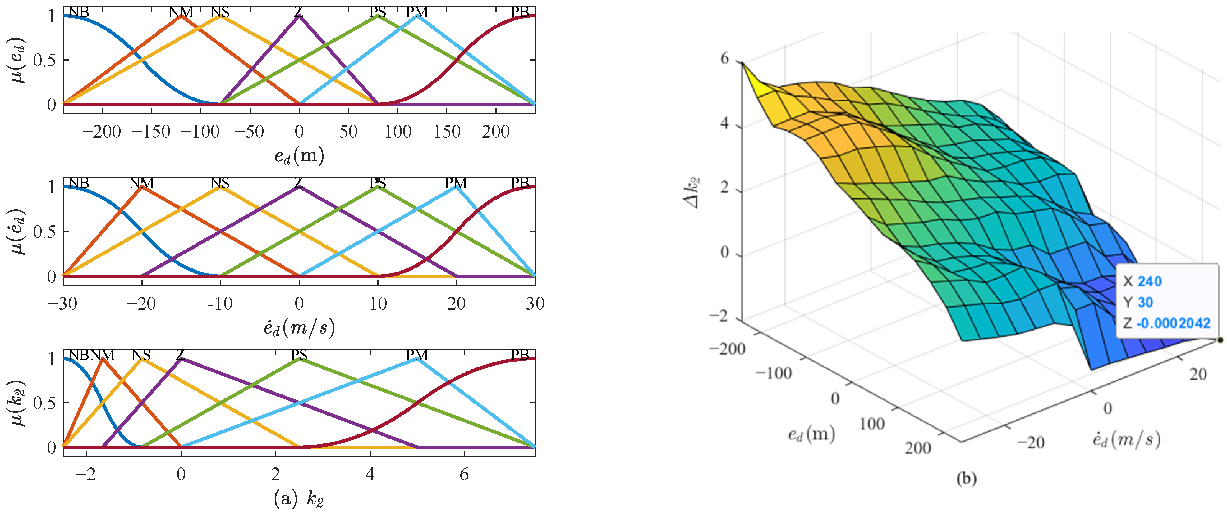
While designing the fuzzy logic controllers, the value of $\Delta k_2$ is defined by the fuzzy rules described in Table 1, based on $e_d$ and ${\dot{e}}_d$. The terms NB, NM, NS, Z, PS, PM, and PB stand for negative big, negative medium, negative small, zero, positive small, positive medium, and positive big, respectively. Figure 7a shows the triangular, Z-shaped, and S-shaped membership functions used for the fuzzification of the inputs $e_d$ and ${\dot{e}}_d$, and the output $\Delta k_2$. The universe of discourse of $e_d$, ${\dot{e}}_d$, and $\Delta k_2$ are given as [−240, 240], [−30, 30], and [−0.00025, 0.00075], respectively. Figure 7b shows the input-output surface for the fuzzy logic controller among $e_d$, ${ė}_d$, and $\Delta k_2$. The minimum value of $\Delta k_2$ is −0.0002042. In this study, the parameter $k_{20}$ is chosen as 0.0008. Then, $k_2$ is always positive with $k_2>0.000596$.

Table 1. Fuzzy rules to estimate $\Delta k_2$, based on $e_d$ and ${ė}_d$.

$\Delta {\mathit{k}}_2$		${\dot{\mathit{e}}}_{\mathit{d}}$
		NB	NM	NS	Z	PS	PM	PB
$e_d$	NB	PB	PB	PM	PM	PS	Z	Z
	NM	PB	PB	PM	PS	PS	Z	NS
	NS	PM	PM	PM	PS	Z	NS	NS
	Z	PM	PM	PS	Z	NS	NM	NM
	PS	PS	PS	Z	NS	NS	NM	NM
	PM	PS	Z	NS	NM	NM	NM	NB
	PB	Z	Z	NM	NM	NM	NB	NB

Figure 7. The properties of the fuzzy controller. (a) The membership functions used for the fuzzification of the inputs $e_d$ and ${\dot{e}}_d$, and the output $\Delta k_2$, respectively; (b) Input-output surface of the fuzzy logic controller among $e_d$, ${\dot{e}}_d$, and $\Delta k_2$.

4. Simulation

The proposed curved-path following control method with adaptive parameters is presented as Figure 8.

Figure 8. The structure of the proposed controller.

The bank-to-turn maneuver with no sideslip is applied to the small fixed-wing UAV. It follows that [25]

$$\dot{\chi }=\frac{\mathrm{g}}{V}\mathit{tan}\left(\varphi \right)$$

(28)

where $\mathrm{g}$ is the magnitude of gravity at sea level. It is assumed that the inner loop PD controller can quickly track the commanded bank angle. At the same time, the dynamics of the bank angle are much faster than those of heading and altitude. In this case, the roll angle can be approximately considered as the commanded bank angle ${\varphi }_{cmd}$. Therefore, Equation (28) becomes

$$\dot{\chi }=\frac{\mathrm{g}}{V}\mathit{tan}\left({\varphi }_{cmd}\right)$$

(29)

Considering the relationship $\dot{\chi }=u_{cmd}$ shown in Equation (1), the bank angle command ${\varphi }_{cmd}$ can be derived as

$${\varphi }_{cmd}={\mathit{tan}}^{-1}\left(\frac{V{u}_{cmd}}{\mathrm{g}}\right)$$

(30)

The simulation was studied in the Matlab/Simulink environment. The Aerosonde UAV model with a wingspan of 2.9 m was used as the test vehicle [29]. Figure 9 shows the simulation in the Matlab/Simulink environment. The parameters used in the simulation are shown in Table 2. The initial $V$ was set as 25 m/s. The sample time was set as 25 ms. A constant wind at 8 m/s from 270° W was also added to the model of the UAV, which will verify the effectiveness of the proposed method under the wind disturbance. The initial position and course of the UAV were set as $\left(0,0\right)$ and 0° N, respectively.

Figure 9. The simulation in the Matlab/Simulink environment.

Table 2. The parameters for simulation.

Parameter	Value	Parameter	Value
Initial V	25 m/s	Wind speed	8 m/s
Sample time	25 ms	Wind direction	270° West
${\mathit{x}}_0$	20 m	$k_{1,ma\mathit{x}}$	$6.0\times {10}^{-4}$
$V_{p1}$	40 m/s	$k_{1,min}$	$3.0\times {10}^{-4}$
$V_{p2}$	15 m/s	$k_{20}$	$8.0\times {10}^{-4}$

4.1. Polygon Path Following

The desired horizontal polygon path was defined with six waypoints: A (0, 0), B (2400, 1386), C (2400, 3386), D (0, 5786), E (−2400, 5786), and F (−2400, 0). The simulation duration is 900 s. Figure 10a shows the comparison of the path following with the control parameter $k_1=k_{1,max}$, $k_1=k_{1,min}$, and $k_{1, adaptive}$. For the convenience of description, the path following controller under the action of $k_1=k_{1,max}$, $k_1=k_{1,min}$, and $k_{1, adaptive}$ is abbreviated as $\mathrm{PFC}\_k_{1,max}$, $\mathrm{PFC}\_k_{1,min}$, and $\mathrm{PFC}\_k_{1,adaptive}$, respectively. To verify the effectiveness of the proposed methods, we compared the path-following performances of the methods $\mathrm{PFC}\_k_{1,max}$, $\mathrm{PFC}\_k_{1,min}$, $\mathrm{PFC}\_k_{1,adaptive}$ and vector field (VF) [20]. While executing the polygon path following, the turn-through-waypoint mode was adopted to switch course.

Figure 10. Comparison of the polygon path following with the four methods $\mathrm{PFC}\_k_{1,max}$, $\mathrm{PFC}\_k_{1,min}$, ${\mathrm{PFC}}_{-}{k}_{1,adaptive},$ and VF. (a) the position; (b) the distance $f\left(x,y\right)$; (c) the parameter $k_1$; (d) the parameter $k_2$; (e) the course rate command $u_{cmd}$; (f) the bank angle command ${\varphi }_{cmd}$.

The response to the straight-line path can be evaluated by the length of the predefined path followed (LOPPF), the convergence distance, and the error overshoot. For a given segment path, the time from the error $f\left(x,y\right)$converging to less than the aircraft’s wingspan until the UAV starts to switch to another path is called the effective time of UAV flying along the given path. The length of the predefined path followed (LOPPF) is defined as the projection length of the UAV’s flight path on the desired segment during this effective path-following time. The convergence time is defined as the time from the UAV following the desired path until $\left|f\left(x,y\right)\right|$ is less than the aircraft’s wingspan. For straight-line path following, the error overshoot is the maximum of $\left|f\left(x,y\right)\right|$, which can be seen in the areas of I, II, III, IV, V, and VI, as shown in Figure 10b.

Figure 10b shows the comparison of the $f\left(x,y\right)$ while following the predefined polygon path with the four methods $\mathrm{PFC}\_k_{1,max}$, $\mathrm{PFC}\_k_{1,min}$, $\mathrm{PFC}\_k_{1,adaptive}$, and VF. As shown in the areas I, II, III, IV, V, and VI, the error overshoots found by using the method $\mathrm{PFC}\_k_{1,max}$ are the largest. The corresponding error overshoots found by using the method $\mathrm{PFC}\_k_{1,min}$ are the second smallest. When using the method $\mathrm{PFC}\_k_{1,adaptive}$, the error overshoots are moderate and closer to those generated by the method $\mathrm{PFC}\_k_{1,min}$. The corresponding error overshoots shown in the areas I, II, III, IV, V, and VI are all listed in Table 3.

Table 3. The performance comparison of the polygon path following using the four methods.

Segment	LOPPF (m)				Convergence Time (s)				Error Overshoot (m)
	${\mathit{k}}_{1,\mathit{m}\mathit{a}\mathit{x}}$	${\mathit{k}}_{1,\mathit{m}\mathit{i}\mathit{n}}$	${\mathit{k}}_{1, \mathit{a}\mathit{d}\mathit{a}\mathit{p}\mathit{t}\mathit{i}\mathit{v}\mathit{e}}$	VF	${\mathit{k}}_{1,\mathit{m}\mathit{a}\mathit{x}}$	${\mathit{k}}_{1,\mathit{m}\mathit{i}\mathit{n}}$	${\mathit{k}}_{1, \mathit{a}\mathit{d}\mathit{a}\mathit{p}\mathit{t}\mathit{i}\mathit{v}\mathit{e}}$	VF	${\mathit{k}}_{1,\mathit{m}\mathit{a}\mathit{x}}$	${\mathit{k}}_{1,\mathit{m}\mathit{i}\mathit{n}}$	${\mathit{k}}_{1, \mathit{a}\mathit{d}\mathit{a}\mathit{p}\mathit{t}\mathit{i}\mathit{v}\mathit{e}}$	VF
AB	2457.48	2236.19	2308.61	2193.64	11.68	18.70	16.38	20.35	--	--	--	--
BC	1462.99	1537.41	1578.74	1486.87	28.13	23.53	21.85	25.83	19.15	4.46	6.46	<0.2
CD	2931.19	3057.74	3080.79	2991.44	28.40	20.28	19.00	24.03	15.39	6.02	8.48	<0.1
DE	1563.01	1685.46	1717.57	1999.72	29.13	20.93	18.93	21.60	13.04	6.12	8.01	<0.1
EF	5339.77	5364.65	5438.53	5258.51	23.58	21.78	18.63	26.80	8.38	1.44	2.29	<0.1
FA	1414.37	1195.11	1316.10	1353.38	23.18	29.40	25.73	25.18	6.12	<0.1	<0.1	<0.1
AB900s	1054.74	1431.50	1369.55	1232.40	14.80	6.90	8.33	12.18	10.82	<0.4	3.17	<0.5

As Figure 10b and Table 3 show, while turning through the waypoint F (2000, 0), the deviations of the UAV from the reference path found by using the four methods are all larger than 125 m, and the largest occur during the first lap flight. These deviations show that, with the two orthogonal components of the added wind acting on the fuselage axis and the lateral axis of the UAV, the wind from 270° W influences the turning of the UAV dramatically. Moreover, the convergence time by using the method $\mathrm{PFC}\_k_{1,adaptive}$ is 25.73 s, which is the longest during the first lap flight. However, the convergence time is moderate by comparing it with those obtained by using the methods $\mathrm{PFC}\_k_{1,max}$ and $\mathrm{PFC}\_k_{1,min}$.

Table 3 lists the performance comparison of the polygon path following using the four methods $\mathrm{PFC}\_k_{1,max}$, $\mathrm{PFC}\_k_{1,min}$, $\mathrm{PFC}\_k_{1,adaptive}$, and VF. The segment AB_900s means that the UAV only follows part of segment AB during the second flight. The LOPPFs when the UAV follows the segments BC, CD, and EF with the method $\mathrm{PFC}\_k_{1,adaptive}$ are the longest. The LOPPFs when the UAV follows the segments AB, DE, FA, and AB_900s are moderate compared with those obtained by the other three methods $\mathrm{PFC}\_k_{1,max}$, $\mathrm{PFC}\_k_{1,min}$, and VF. During the 900s’s flight, the total LOPPFs by using the methods $\mathrm{PFC}\_k_{1,max}$, $\mathrm{PFC}\_k_{1,min}$, $\mathrm{PFC}\_k_{1,adaptive}$, and VF are 16,223.55 m, 16,508.06 m, 16,809.59 m and 16,515.96 m, respectively. This indicates that the UAV can fly on the most desired polygon path by using the method $\mathrm{PFC}\_k_{1,adaptive}$.

4.2. Circular Path Following

Figure 11a shows the position comparison while following the circular path using the three methods. The desired circular path is defined as two concentric circles with circle A: $\sqrt{x^2+{\left(y-350\right)}^2}-250=0$, and circle B $\sqrt{x^2+{\left(y-350\right)}^2}-350=0$. The UAV first flew toward circle A. About 180 s later, the UAV started to switch from the position (0, 600) and flew toward circle B with a radius of $350 \mathrm{m}$.

Figure 11. Comparison of the circular path following using the four methods $\mathrm{PFC}\_k_{1,max}$, $\mathrm{PFC}\_k_{1,min}$, ${\mathrm{PFC}}_{-}{k}_{1,adaptive},$ and VF. (a) The position; (b) the distance $f\left(x,y\right)$; (c) the parameter $k_1$; (d) the parameter $k_2$; (e) the course rate command $u_{cmd}$; (f) the bank angle command ${\varphi }_{cmd}$.

The distance $f\left(x,y\right)$ presented in Figure 11b shows that, with the parameter $k_1$ adaptive, the method $\mathrm{PFC}\_k_{1,adaptive}$ inherits the advantages of the rapidity of the method $\mathrm{PFC}\_k_{1,max}$ and the small overshoot of the method $\mathrm{PFC}\_k_{1,min}$. The error overshoots of $f\left(x,y\right)$for the first circular path following using the three methods $\mathrm{PFC}\_k_{1,max}$, $\mathrm{PFC}\_k_{1,min}$, and $\mathrm{PFC}\_k_{1,adaptive}$ are 22.65 m, 11.07 m and 12.52 m, respectively. When switching to fly toward circle B, the error overshoots of $f\left(x,y\right)$using the methods $\mathrm{PFC}\_k_{1,max}$, $\mathrm{PFC}\_k_{1,min}$, and $\mathrm{PFC}\_k_{1,adaptive}$ are 14.59 m, 2.25, and 3.03 m, respectively.

The length of the predefined circular path followed (LOPCPF) is defined as the length of the actual flight path after the time that the UAV has converged to the desired circular path. Table 4 lists the LOPCPF, the convergence time, and the error overshoot for the UAV to follow the two circles A and B. It is determined that it takes only 10.60 s for the UAV to converge to circle B using the method $\mathrm{PFC}\_k_{1,adaptive}$. While using the methods $\mathrm{PFC}\_k_{1,max}$ and $\mathrm{PFC}\_k_{1,min}$, the convergence times are 20.95 s and 14.83 s, respectively. During the 300 seconds’ flight, the LOPCPF by using the three methods $\mathrm{PFC}\_k_{1,max}$, $\mathrm{PFC}\_k_{1,min}$, $\mathrm{PFC}\_k_{1,adaptive}$, and VF are 5356.88 m, 5662.37 m, 5742.11 m, and 5879.15 m, respectively. The above indicates that the method $\mathrm{PFC}\_k_{1,adaptive}$ will still cause the UAV to fly the second most accurately on the desired circular path, with moderate convergence time and error overshoot.

Table 4. The performance comparison of the circular path following using the four methods.

Circle	LOPCPF (m)				Convergence Time (s)				Error Overshoot (m)
	${\mathit{k}}_{1,\mathit{m}\mathit{a}\mathit{x}}$	${\mathit{k}}_{1,\mathit{m}\mathit{i}\mathit{n}}$	${\mathit{k}}_{1, \mathit{a}\mathit{d}\mathit{a}\mathit{p}\mathit{t}\mathit{i}\mathit{v}\mathit{e}}$	VF	${\mathit{k}}_{1,\mathit{m}\mathit{a}\mathit{x}}$	${\mathit{k}}_{1,\mathit{m}\mathit{i}\mathit{n}}$	${\mathit{k}}_{1, \mathit{a}\mathit{d}\mathit{a}\mathit{p}\mathit{t}\mathit{i}\mathit{v}\mathit{e}}$	VF	${\mathit{k}}_{1,\mathit{m}\mathit{a}\mathit{x}}$	${\mathit{k}}_{1,\mathit{m}\mathit{i}\mathit{n}}$	${\mathit{k}}_{1, \mathit{a}\mathit{d}\mathit{a}\mathit{p}\mathit{t}\mathit{i}\mathit{v}\mathit{e}}$	VF
A	3464.27	3598.88	3585.89	3725.95	28.40	22.65	22.28	14.98	22.65	11.07	12.52	<0.1
B	1892.61	2063.49	2156.22	2153.20	20.95	14.83	10.60	11.00	14.59	2.25	3.03	<1

5. Conclusions

This paper has considered the problem of horizontal curved-path following using fixed-wing UAV. The guidance strategies are derived using a kinematic model of the aircraft and using the Lyapunov stability theory. The control parameters in the guidance law are time-varying and adaptive to the initial states and dynamics of the corresponding nonlinear system. The rules of the time-varying P-like parameter are designed by using an exponential equation shown as (15), where its corresponding parameter $\tau$ is determined by using the fourth order Runge–Kutta algorithm and the bilinear interpolation method. The rules of the time-varying D-like parameter are designed based on the fuzzy logic technique. The stability of the corresponding nonautonomous nonlinear system is also guaranteed. Finally, we have demonstrated the effectiveness of the proposed strategies in a Matlab/Simulink simulation environment with an Aerosonde model. For the given square and circular paths, the method using the adaptive parameters can make the UAV fly more accurately on the target path based on the performance indexes LOPPF and LOPCPF. In the sense of path following, the proposed method provides a methodology that will be applied to realize the better path following of unmanned systems, including aerial, underwater, and ground-based robots.

In the actual flight process, the roll angle command is bounded, which should be considered in the parameter design of the controller. At the same time, if the bank angle command tracking control response of the UAV is very fast, the method described in this paper will be effective. If its response takes a certain time, the closed-loop roll dynamics must be considered in the design of controller. The closed-loop roll dynamics can be expressed as a first-order system. The follow-up research work will further design the path following controller by using the backstepping technique.

In the future, the closed-loop roll dynamics of the bank angle presented by a first-order system with the unmodeled parts will be used to generate the bank angle command in order to make the vehicle follow the predefined path more precisely. The method to estimate the disturbance described in [28] will also be considered to design a robust controller.