Abstract
The paper deals with the proposed concept of a biped robot with vertical stabilization of the robot’s base and minimization of its sideways oscillations. This robot uses 6 actuators, which gives good preconditions for energy balance compared to purely articulated bipedal robots. In addition, the used linear actuator is self-locking, so no additional energy is required for braking or to keep it in a stable position. The direct and inverse kinematics problems are solved by means of a kinematic model of the robot. Furthermore, the task is aided by a solution for locomotion on an inclined plane. Special attention is focused on the position of the robot’s center of gravity and its stability in motion. The results of the simulation confirm that the proposed concept meets all expectations. This robot can be used as a mechatronic assistant or as a carrier for handling extensions.
1. Introduction
Humanoid bipedal robots have been attracting the attention of researchers around the world for several decades. Leonardo da Vinci is considered to be the creator of the first humanoid robot, although the WABIAN-2 robot from Waseda University is considered to be the first humanoid walking robot [1,2,3].
Research in the field of bipedal robots focuses on several areas, namely research on artificial intelligence, research on human–robot interactions, and research on the implementation of bipedal locomotion and hardware development. As this is a complicated issue, many research teams are focusing on these problem areas of humanoid robotics [1,4,5,6,7].
Many scientific issues in this area need to be solved, such as issues related to the optimal kinematic and dynamic modeling of robot design, process control, balance control, navigation, path planning, actuator control, robot position sensing, energy efficiency optimization, decision making, and many other factors [8,9,10,11,12,13,14,15,16].
Bipedal robots are destined to perform many routine activities performed by humans. Humanoid two-legged interactive robots are generally designed for entertainment, communication (social activities), guidance, education, health care, mental therapy, personal assistance, house cleaning and maintenance, and other purposes [17,18,19,20].
Some studies have used the knowledge of double-legged locomotion to reduce the energy costs of the person performing the work by using exoskeletons. These exoskeletons help people to perform difficult tasks and can also help those who are unable to do so for health reasons [21,22,23,24,25].
One perspective area of application of biped locomotion involves the use of prosthetic legs or leg parts such as the ankle joint for walking, as proposed in [26,27].
Conventional biped systems are designed to be highly functional and versatile, but are often disproportionately slow, dangerous, or expensive to implement due to the bipedal locomotion approach. The performance of traditional two-legged robots is often limited by their design, having a high number of degrees of freedom (DoF) and complicated control. The large number of joints in the robots makes their modeling and motion control complicated. One possible solution is to abandon the conventional humanoid paradigm and create a non-anthropomorphic robot concept, with better mobility and a lower DoF [28,29,30].
This paper deals with the concept for a bipedal robot, diverging from the conventional articulated humanoid concept and involving an unconventional arrangement of the robot. This concept can be used for the construction of a mechatronic assistant, which would help people in normal work at home, in industry, or in patient care, where it would also allow the transport of patients.
2. Related Work—Literature Review
A previous paper [16] presented a modified passive walking model for flexible legs, involving a pair of elastic beams with small deflections instead of the usual rigid links. The main contributions of this paper lie in the modeling of the impulsive hybrid dynamics of flexible passive bipeds and the application of a numerical technique based on a finite difference formula to find the appropriate initial conditions for walking gait cycles. The authors of [9] proposed a foot swing trajectory generation method for biped walking, aiming to minimize the velocity and acceleration of leg swing for an anthropomorphic biped robot concept with many degrees of freedom. With the simplified optimization model proposed in their paper, a fast offline foot swing trajectory generation was achieved. Experiments involving the BHR6 biped robot demonstrated the effectiveness of the proposed method, where walking at a speed of 4 km/h was achieved with the optimized foot swing trajectory. Another paper [28] introduced the non-anthropomorphic Biped: Version 2 (NABi-V2), a bipedal robot that is a departure from the conventional humanoid paradigm in its morphology and actuation method; that is, NABi-V2 is a platform with a unique leg configuration that is designed around high-torque back-drivable electric actuators that provide proprioception and force control capabilities. Another study [8] proposed a new stability criterion for biped walking systems based on a linear inverted pendulum model, in which the dynamic relationship between the center of mass and the zero-moment point was covered. More precisely, based on the fact that a biped walking robot is stable if its zero-moment point is always located in the supporting region, the authors considered whether the ZMP error between its reference and real values stays inside a certain area to guarantee the stability condition.
When a humanoid biped robot walks on a sloping plane in an arbitrary direction, the right leg flexion is different to that of the left leg. In this way, the orientation of the torso is obtained to preserve the equilibrium of the humanoid robot during walking. In such cases, the specification of the required 3D motion of the pelvis and feet becomes a quite complex issue. To solve this problem, in this paper a general and simplified formulation was proposed and applied to obtain a cycloidal walking pattern for a humanoid robot. A bioloid humanoid robot is analyzed in the paper [31] is based on a cycloidal motion of a humanoid on a sloping surface. In another paper [30] the authors presented the gyrubot biped robot. It has two DoF legs and two scissored pair control moment gyroscopes. The gyrubot is an original mechanical design for a 3D bipedal robot based on augmentation with multiple control moment gyroscopes [30].
The CRANE robot is an underactuated, torque-controlled 3D bipedal robot. The robot has a torso and two legs. There is a control computer, battery, and inertial measurement unit inside the body. The robot has actuators that are placed very high, and overall the center of gravity is very high [12].
A previous paper [13] introduced a new gait switching approach for an underactuated biped walker named ERNIE. The switching condition relies on a reduced region of attraction—that of the unactuated dynamics—which is shown to be sufficient to predict falls. Fully actuated biped robots with powered ankles often rely on the zero-moment point principle to guarantee that the robot does not fall, typically prioritizing robustness over energetic efficiency. In contrast, underactuated bipeds exploit the same natural dynamics of human locomotion to offer the promise of efficiency, but have limited ability to reject large disturbances in their unactuated DoF. A previous study [14] described a control method for the stable standing and walking of a bipedal robot based on inertial measurement unit sensor feedback. The inertial measurement unit sensor was used to measure the tilt posture of the robot in uneven terrain conditions. In this paper, an indication of bipedal walking stability was determined based on the tilt posture of the robot body. The performances of the proposed methods were verified via walking experiments using a 18-DOF biped robot, El Pistolero. The authors of [15] imitated humans’ ability for slope angle perception. Using Kinect sensors to obtain the walking information of the human body under different slopes, and then using a long short-term memory neural network to jointly learn the degrees of freedom of multiple lower limb joints, the classification and recognition of different slopes was completed, then the robot’s ankle joints were compensated based on the slope inclination. On the WEBOTS simulation platform, the biped robot NAO is driven to reproduce the walking action in a slope environment according to the corresponding movement strategy and the label compensation method is obtained according to the classification. BRZ-4 is a half-size biped robot, which was set up as a test bed in [32]. It is a standard joint concept composed of a 3D-printed mechanical structure driven by Dynamixel motors. In total, it has 17 DoF joints. The authors developed a new online walking controller for biped robots, which integrates a neural network estimator and an incremental learning mechanism to improve the control performance in dynamic environments.
In the biped robotics domain, head oscillations may be extremely harmful, especially if the robot is teleoperated, since vibrations strongly reduce the operator’s spatial awareness. In particular, undesired head oscillations occur in underactuated robots, whereby springs and passive mechanisms are used to achieve human-like motion. The authors of [33] proposed an approach to reduce the vibrations of a biped robot’s head; the proposed solution does not affect the dynamic locomotion properties on which a specific control logic could have been tuned. The approach was tested on Rollo, a flexible, wheeled biped robot, whose head vibrates throughout the robot locomotion.
The authors of [34] proposed a gait pattern with torso pitch motion control during walking. Additionally, they presented a gait pattern while keeping the torso vertical to study the effects of torso pitch motion on the energy efficiency of biped robots. They defined the cyclic gait of a five-link biped robot with several gait parameters. The gait parameters were determined via optimization. A five-link planar biped robot with knees was used as the model for the analysis and the cyclic gait of a five-link biped robot was designed. The disturbance rejection performance of a biped robot when walking has long been the focus of roboticists in their attempts to improve robots. There are many traditional stabilizing control methods, such as modifying foot placements and the target zero-moment point, e.g., in model zero-moment point control. The disturbance rejection control method in the forward direction of the biped robot is an important technology, whether it comes from the inertia generated by walking or from external forces [35].
A previous study [36] presented a novel framework for a hydraulic-driven biped robot. The target biped robot was a humanoid robot named NWPUBR-1 with 12 DoF, and its dimensions were close to those of an average male. The joint axis involved a modular sensor allowing angular measurements, and the force sensor was deployed on the side of the hydraulic actuator to facilitate force and position control of the robot. To achieve real-time control of the robot’s gait in 3D space, a three-dimensional linear inverted pendulum model was built and a 3D gait model was generated by combining the zero-moment point theory.
The LARMbot humanoid robot was developed at the Laboratory of Robotics and Mechatronics of the University of Cassino. It was designed as a low-cost, user-friendly humanoid robot for service tasks, featuring parallel mechanisms both in its legs and torso to achieve high kinematic and dynamic performance. This humanoid robot was characterized by 22 active DoF [37].
Another study [38] presented a simple idea for a 4 degree of freedom (DOF) walking robot with the ability to walk on flat surfaces, rotate, and climb upstairs, which was composed of vertical moving legs with a rotary foot and a controlled mass to allow stabilization. A prototype model of a 3-DOF walking robot was presented for walking only on flat surfaces. This walking robot was actuated by servomotors. The paper covered the kinematics, a center of gravity analysis, a description of the robot, and its control system, which involved a Pololu controller. The experiments confirmed the feasibility of the proposed design.
Most of the relevant studies have dealt only with the movement and stability of robots, but do not address the vertical stabilization of the base. This work is different in that it focuses on the design of suitable robot kinematics that will be more advantageous in stabilizing the robot’s base. By following such a design, control will also be easier, as poorly designed kinematics will cause complications in locomotion control. Some studies have dealt with vertical stabilization by controlling the movement rather than the structure itself [39,40].
The rest of this paper is organized as follows. Section 3 describes the aims and motivations for this work. Then, we outline our robot concept in Section 4 and build a kinematic model for our concept in Section 5. These direct kinematic and inverse kinematic models are usable for control of the robot on inclined planes. Section 6 deals with the stability of the robot, including on an inclined plane. The walking simulation results are presented in Section 7. A discussion and directions for future work are presented in Section 8. Section 9 concludes this paper.
3. Aims and Motivation for This Work and Technical Contributions
The aim of this work is to create a biped walking robot that meets the following requirements:
- To design such a biped robot so that its method of walking does not require tilting the base to the sides;
- To ensure a constant height of the robot’s base from the ground when walking;
- If necessary, simple adjustments of the height of the robot’s base from the ground should be possible;
- The robot should have the ability to walk on an inclined plane;
- The use of low-cost actuators should be considered;
- As few actuators as possible should be used in the robot design.
It is quite complicated to meet these requirements using a biped anthropomorphic robot, so the aim of this work is to explore the possibility of applying non-anthropomorphic concepts for use in two-legged locomotion.
The aim of this work is to create a mathematical model of a robot using direct kinematics and an inverse kinematic model, which can be used for the purpose of controlling robot actuators and for simulations to verify the proposed concept. Since stability is a serious problem in double-legged locomotion, the aim is also to assess the stability of the proposed robot concept. In terms of stability, the goal of the design is to place the overall center of gravity of the robot as low as possible.
The aim of this concept is to use as few actuators as possible and to reduce the total weight of the robot, as well as the energy requirements for the operation of such a robot. The use of many actuators would mean more weight but also more energy consumption and a short range or operation.
By applying non-anthropomorphic principles, it is possible to achieve a certain degree of self-locking of the individual joints, which will also enable energy savings, which would otherwise need to be used to maintain the robot in a stable state.
Three main contributions of this work can be summarized as follows:
- (1)
- The creation of a new two-legged non-anthropomorphic robot capable of overcoming obstacles while its base is vertically stabilized. The base of this robot will provide space for sensor systems and handling equipment;
- (2)
- The robot’s base is stabilized to allow movement on an inclined plane, both for ascending and descending terrain;
- (3)
- Simulation experiments are performed on a scaled-down model using the parameters of real actuators, while the aim is to examine the potential of the proposed concept. In the future, however, it will be possible to adapt this concept to larger dimensions and implement mobile platform for people with disabilities, providing a better ability to overcome terrain obstacles in urban environments. Another possibility is the creation of a mechatronic assistant to help people in the work environment, in the care of patients, or possibly as a home personal assistant.
4. Proposed Robot Concept
The robot is designed as a biped, single-axle robot, which means that the legs of the robot are placed in parallel (Figure 1). The walking motion is designed so that the feet are overpassed, so that it is not necessary to transfer the center of gravity of the robot by tilting the robot to the sides. While walking, at least one of the feet is always in contact with the ground, so there is no so-called flight phase.
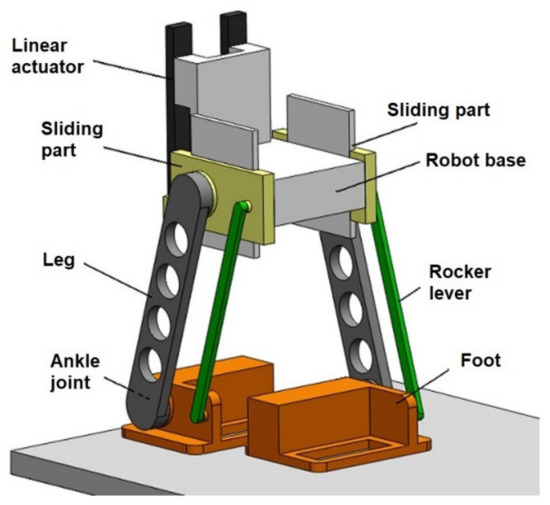
Figure 1.
Model of the designed biped robot concept.
The robot design involves a combination of a linear connection and a parallelogram, which aims to create a permanent parallel relationship between the feet and the base of the robot (Figure 1). The robot consists of four planar rotary joints and two equally long parallel rocker levers. The rotary oscillating movement of this mechanism is ensured by a rotary actuator located in the robot’s foot, meaning the resulting center of gravity of the robot is as low as possible. A linear actuator is used to drive the linear link, which adjusts the vertical position of the parallelogram (Figure 1). The advantages of this concept also include the easy adjustment of the height of the robot’s base by means of simultaneous insertions or retractions of linear drives. In order to be able to turn the robot sideways, the design is supplemented by a solution that allows one to change the direction of walking. Two other rotary actuators are used for this, which rotate the rotating pads located under the feet (Figure 2). In total, this robot concept requires only 6 actuators, which is a smaller number of actuators than in other existing biped robot concepts.
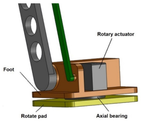
Figure 2.
The concept of a rotating foot to change the walking direction.
Human-like anthropomorphic robots have very complicated kinematics, many degrees of freedom, and many actuators. Therefore, these robots weigh a lot and require complicated control systems. It is even more complicated to maintain the robot’s base at a constant height without tilting the body to the sides.
The non-anthropomorphic bipeds used in this work have different kinematics than for humans, making it easier to achieve double-legged locomotion using fewer actuators. To achieve vertical stabilization, only one linear actuator is needed for each leg. The use of multiple actuators would significantly slow down the robot’s locomotion and increase the robot’s size. A thorough analysis of locomotion concepts preceded this robot design. Several concepts have been developed and energy requirements were investigated using SolidWorks simulations with the Power Consumption feature. The concept solved in this article was evaluated as the best in terms of consumption energy.
A linear slider–rotary joint combination is chosen here for this concept. It is also possible to use a linear slider–linear slider combination, but this would mean that the speed of the robot’s movement would be significantly reduced. Linear drives with electric motors are slower than articulated drives and the use of two linear drives would require rapid deceleration during robot locomotion. Therefore, a linear slider–rotary joint is chosen here.
The used non-anthropomorphic concept also has advantages compared with wheeled, tracked, and quadruped concepts. Wheeled and tracked undercarriages copy the terrain during locomotion and cannot stabilize the robot’s base vertically, as this would require an additional steering mechanism. The animal-inspired quadruped locomotion is achieved using articulated kinematic structures with center of gravity transfer by tilting and transferring the center of gravity to the supporting polygon formed by the legs. The complexity of the quadruped concept means it is not suitable for vertical stabilization of the robot’s base.
One of the requirements in the design is to consider the use of available inexpensive rotary and linear actuators. Thus, specific actuators are selected for this concept. Rotation angle sensing for rotary servomotors and extension sensing for linear servomotors are achieved by means of resistance sensors integrated directly into the given actuators. The quantities are determined using a command in the control program. If necessary, the actuators can be modified and wires can be connected directly to the resistance sensors in the actuators, meaning the current position signal can be given to the control unit. This position information can then be used to control the robot’s movement. The contact of the robot’s foot with the terrain is detected using touch sensors. Thanks to this information, it is possible to evaluate whether the robot is standing on one foot, on both, or whether the robot has overturned. Thanks to the proposed kinematics, this resulting concept (Figure 3) meets the specified requirements.
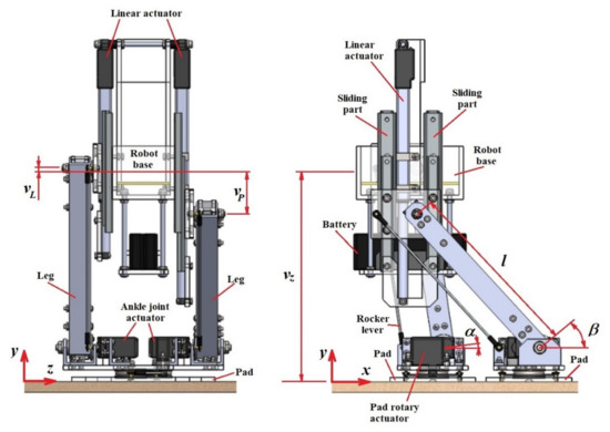
Figure 3.
The final design of a biped walking robot.
5. Robot Kinematics
To design a robot walking algorithm and to maintain its stability, it is necessary to know the exact positions of individual parts of the robot (Figure 4). For this reason, the issue of robot kinematics is solved in this chapter. The kinematics of spatial mechanisms contains two basic tasks, namely the direct kinematics and the inverse kinematics. In the kinematics of mechanisms with moving members, it is very appropriate from a practical point of view to describe their mutual position using a system of local coordinate systems, which are firmly assigned to individual links and move with them at the same time. Their position and orientation in relation to the global coordinate system can, thus, be easily determined. The individual generalized coordinates are then defined on the basis of the local coordinate systems as angles and oriented distances between the given axes of the local systems.
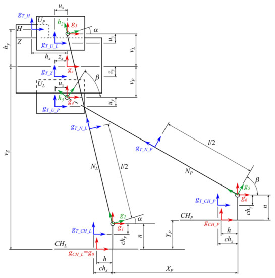
Figure 4.
Simplified model of the designed biped walking robot in the x-y plane. All symbols are described below.
The symbols and abbreviations used in the kinematic model are as follows:
CHL, CHP, NL, NP, UL, UP, Z, H—main parts of a biped robot;
chX, chY, uX, uY, zX, zY, hX, hY—constants defining the position of the centers of gravity of individual parts;
α, β, vL, vP—generalized coordinates;
n, h, l—dimensional constants;
g…, h…—local coordinate systems of the main points of the kinematic chain;
gT…—local coordinate systems of the centers of gravity of individual robot parts;
vZ, XP, YP—base height and position of the robot’s right foot position.
A necessary part of the analysis of this robot is a complete kinematic model of the mechanical system, which will provide us with all of the important kinematic quantities. The positions of individual articles are generally described by generalized coordinates (joint variables). In our kinematic model of a walking robot shown in the x-y plane, the generalized coordinates of the Hitec HS-645MG motors are determined by the angles α and β and extrusions of Firgelli L12 linear motors, denoted as vL and vP, respectively (Figure 4).
5.1. Direct Kinematic Model of a Robot
In direct kinematics, a problem is solved when generalized coordinates are known with consideration of n as the joint space dimension, and it is necessary to determine the positions and orientations of individual parts of the mechanism with m as the number of tasks in the space dimension. This problem is relatively easily solved using trigonometric relations between individual members or using local coordinate systems of members using transformation matrices to convert coordinates between them. Since a firmly anchored kinematic chain is assumed, the center of the contact surface of the left foot of the robot in the diagram is at the beginning of the reference coordinate system g0 (Figure 4) and the positions of the other parts are derived from this position. The diagram (Figure 4) also contains coefficients specifying the positions of individual centers of gravity, which are important in calculating the position of the overall center of gravity of the robot and in assessing its stability.
A special Euclidean group SE (2) is used to calculate the kinematic chain of the robot, which contains rotation and translation. An example is the element with components (x, y, ϕ) belonging to SE (2), which is represented by a homogeneous matrix:
The solution is to gradually add more members of the mechanism to the original systems:
After recalculating the positions and orientations of the coordinate systems of the main points of the kinematic chain, the next solution is oriented to the coordinate systems of the centers of gravity of the individual parts of the walking robot. For this purpose, it is necessary to know the location of the centers of gravity with respect to the corresponding main points of the chain. These distances define the values of chx, chy, ux, uy, zx, and zy, the exact dimensions of which can be easily deduced from the created robot model in SolidWorks.
5.2. Direct Kinematic Model with Inclined Plane Consideration
Among the advantages of the proposed robot concept is its ability to walk on a plane that has a certain ascent or descent in the walking direction. This ascent or descent is actually the rotation of the coordinate system g0 at its origin around the z-axis. The rotation is determined with respect to the coordinate system gG by the angle ϕ, which is shown in Figure 5.
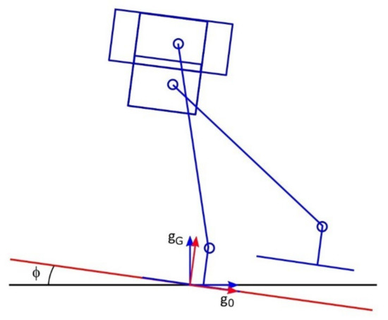
Figure 5.
Tilting the plane in the walking direction.
The following matrix expresses the relationship between coordinate systems g0 and gG:
When solving the direct kinematics problem without considering the inclination of the plane, the coordinate system g0 is the reference and the other parts of the mechanism are recalculated to this system. If we consider the inclination of the plane, it is necessary to recalculate all positions of the key points of the kinematic chain and the positions of the centers of gravity of the individual parts with respect to the new base coordinate system gG, whose y-axis is parallel to gravity. Rules based on the characteristics of operations used by Lie’s group and their actions are re-used for this task:
Subsequently, the positions of the centers of gravity of the individual parts of the robot with respect to the coordinate system are recalculated gG:
5.3. Inverse Kinematics
The inverse kinematics problem involves the basic calculation of the kinematics of mechanisms, which is essential for the purpose of positioning the individual members of the mechanism. This involves an inverse transformation of a complex position vector into a general coordinate vector , the component of which is the coordinates of the rotation or displacement of individual kinematic pairs.
The inverse transform vector method, which is suitable for kinematic chains with a small number of degrees of freedom, is used here to solve the inverse kinematics of a walking robot. It is based on trigonometric relationships between members, using vector and matrix calculations to complete them. Problem solving using this method is easy and very fast, and this method is often used for real-time positioning. The inverse kinematics task is performed for movement on a plane without considering tilt. Matrices are used as starting points for the calculation, which determine the position and orientation of the coordinate systems of the main parts of the kinematic chain and are calculated using Equations (2) to (11).
The calculation of generalized rotation angle coordinates α is derived from the position of the coordinate system gZ, g0 and the base height value vZ:
Another solution is to use the position of the coordinate system gCH_P,g0 and the mutual distance of the feet xP:
It is also possible to derive a generalized coordinate from Equation (41) as β:
The value of the generalized linear motor position coordinate vL is based on the position matrix for the coordinate system gZ,g0 and the base height from the base vZ:
The matrix gCH_P,g0 (11) and the height of the right foot above the pad yP are used to derive the vP coordinate. Subsequently, Equation (45) expressing the left motor extension vL is inserted into Equation (46):
6. Stability of the Biped Walking Robot
The degree of static stability is represented by the smallest distance of the center of the gravity projection from the boundary of the supporting base, similarly to human gait. Other factors include the weight of the body, the size of the support base itself, and the height of the center of gravity from the base.
By analogy, as the stability is divided, the walking modes of biped robots are also divided into static and dynamic:
- Static walking—the walking robot is statically stable at all times, even if the walking is interrupted at a certain stage of the step. The main disadvantage is the significantly limited walking speed, as it is necessary to eliminate the dynamic effects;
- Dynamic walking—the walking robot is dynamically stable, so the robot does not have to be statically stable at every stage of the step to maintain balance. Therefore, it is necessary to know the exact positions of individual parts of the robot’s kinematic chain, their speed, and their acceleration during this type of walking, which significantly increases the requirements for the control system. However, the advantage is smoother, more natural, and much faster movement of the robot.
Most walking robots have several support points of contact with the pad during walking to ensure permanent stability. However, with two-legged robots, only one foot is in contact with the pad during the step phase, i.e., at higher speeds, the biped robot becomes statically unstable, so if it does not walk significantly slowly it must perform a dynamic gait.
The area on which the foot surface comes into direct contact with the pad is called the area of contact. Part of this area is the area of support, which is used to form a support base. The base of support is the area defined by the outermost boundaries of the support area [41].
In the step phase of a biped robot, when only one foot is in contact with the pad, the support base is the area bounded by the boundary points of the robot’s foot. If the robot is standing on both feet, the support base is a polygon with the smallest possible circumference, which includes all boundary points of both feet.
Due to the strict requirements for the control system and the complexity of controlling the dynamic gait of a robot, the aim of this work is to solve the problem of static walking. With this type of walking, it is necessary to ensure the constant static stability of the robot during each phase of the step and to minimize possible dynamic effects by limiting the speed and acceleration of the actuators. The degree of static stability of the walking robot is essentially influenced by the distance of the vertical projection of the robot’s center of gravity from the edge of the support base. Therefore, the center of gravity is placed as close as possible to the center of the support base.
Since the feet of the proposed walking robot are overpassed, the position of the z-axis coordinate projection from the center of gravity in the supporting base of the robot is always ensured in all circumstances. For this reason, the suitable positioning of the center of gravity projection is focused on the x-axis component of the robot’s center of gravity.
The following formula is used to calculate the x-axis of the center of gravity of the system of mass points:
where: m—total mass of the system of mass points, mi—mass of individual mass points, xi—position of individual mass points.
The positions of the centers of gravity of the individual parts of the robot obtained from Equations (12) to (19) as well as the corresponding weights are calculated as follows:
From Equation (52), the term lsinβ is expressed, which is then substituted into the previous Equation (53):
This procedure provides a relationship to calculate the angle α without the need to know other generalized coordinates. It is necessary to enter the variable xT used to define the desired x-coordinate of the position of the total center of gravity of the robot and the variable xP, which expresses the mutual distance of the feet. The overall robot configuration is obtained by calculating the generalized β, vL, and vP coordinates using the inverse kinematics equations (43), (45), and (48).
6.1. Stability on an Inclined Plane
If the plane is tilted and the coordinate system g0 is rotated with respect to the coordinate system gG by an angle ϕ, it is necessary to shift the total center of gravity by a distance xN in order to maintain the static stability of the robot. Since the center of gravity projection is performed in the direction of the gravitational action vector and the y-axis of the gG coordinate system is parallel to this action, this offset ensures the correct position of the center of gravity projection in the robot support base (Figure 6).
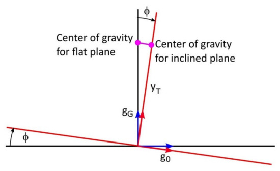
Figure 6.
Necessary shift of the center of gravity to maintain the stability of the robot.
Subsequently, we can substitute yT into the equation, which we obtain from the relation to the calculation of the y-component of the center of gravity of the system of mass points:
The positions of the centers of gravity of the individual parts of the robot are set from Equations (12) to (19):
The equation needs to be modified so that it contains only the generalized coordinate α. Equations (45) and (46) from the inverse kinematics are modified and substituted for this purpose:
The generalized vP coordinate still remains in the equation, which if we express using the angle α we obtain the following relation from the robot kinematics:
Substituting this relationship into Equation (64) would complicate the derivation of the generalized α coordinate, so it is preliminarily considered to neglect the vp coordinate.
Subsequently, the relation for calculating yT is inserted into Equation (55) and the resulting displacement xN is subtracted from the center of gravity xT by substituting it into relation (54):
The following substitutions are used to simplify the following adjustments:
The simplified relationship after the introduction of substitution has the following form:
After the introduction of further substitutions in (73) and (74), the resulting relationship is obtained in Equation (75):
In Equation (75), it is possible to use the trigonometry rules to replace the cos α term as follows:
Substituting Equation (76) into Equation (75) gives the following:
Since in the resulting relation (78) the absolute values arise after exponentiation of the members H and G, the use of this relation to calculate the generalized α-coordinate is limited:
The other generalized β, vL, and vP coordinates are determined using inverse kinematics relations (43), (45), and (48). After this recalculation, the overall stable configuration of the walking robot is obtained.
6.2. Calculation of Stable Robot Configuration
The calculation itself is performed to check the relationships derived in the chapters focused on the kinematics and stability of the robot and also to obtain the necessary data to create simulations of the robot when walking on a flat surface, inclined surface, and in overcoming obstacles.
The MATLAB software environment is used to create a program to recalculate the robot’s configuration. The calculation is performed for specific input values of the position of the second foot (xP, yP), the height from the base (vZ), the x-position of the total center of gravity of the robot (xT), and the angle of inclination of the plane (ϕ). The task involves calculating the generalized coordinates of the walking robot, namely α, β, vL, and vP. For this calculation, we use the equation to determine the angle α (78) derived in the chapter on robot stability. However, there is a term G in this equation that contains the generalized vP coordinate. Since this value before the calculation of angle α is not known and its replacement by the expression from Equation (64) is complicated, the calculation is performed twice using the M-file. In the first calculation, the vP coordinate is neglected and its value is set to zero. From the obtained value of the angle α, the other coordinates are subsequently recalculated using the inverse kinematics Equations (43), (45), and (48). However, the center of gravity of this robot configuration has a deviation of ±1 mm from the setpoint due to neglecting vP. To obtain better accuracy, the calculation of the generalized α coordinate is performed a second time and the value from the previous calculation is substituted for the vP member. This is followed by recalculating the other β, vL, and vP coordinates to obtain the overall robot configuration. The deviation of the center of gravity from the required position after recalculation is within ±0.1 mm. If the inclination of the plane is not considered in the calculation, then the term G is equal to zero and the center of gravity of the resulting configuration corresponds to the required value after the first recalculation.
Furthermore, the positions of the individual parts of the robot’s kinematic chain are calculated using the relations from direct kinematics with consideration of the inclined plane ((21) to (30)) and subsequent substitution of the generalized coordinates α, β, vL, and vP, which have been recalculated before. The actual position of the center of gravity CoG is also determined in this program, which is further recalculated to the x-value of the center of gravity with respect to the coordinate system g0.
Subsequently, the robot’s motion is plotted in a graph. For this, matrices with positions of individual parts of the robot from Equations (21) to (30) are used and the corresponding shapes are drawn around these points. The graph also shows the center of gravity of the robot, the actual x-position of the center of gravity with respect to the coordinate system g0, and the current values of the generalized coordinates. The following figures show the basic configurations of the robot in different phases of locomotion when walking on a flat surface (Figure 7), on a base with a slope of 8° (Figure 8), and on a base with a slope of −8° (Figure 9).
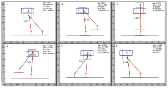
Figure 7.
Plotted configurations of the robot when walking on a flat surface. Legends: 1—the center of gravity of the robot is above the right foot; 2—the left linear actuator performs the upward stroke of the left foot; 3—the left ankle joint rotates to move the left foot forward and at the same time the right ankle joint balances the robot’s pose to the vertical position of the legs; the right linear actuator also works to keep the base at a constant height; 4—the left ankle joint transmits the left foot forward and at the same time the left linear actuator lowers the foot; the right linear actuator also lifts the base to keep it at a constant height. 5—the left foot is lowered to the ground; 6—both ankle joints rotate so that the center of gravity is transferred above the left foot and at the same time the height position of the base is compensated by the movement of both linear actuators.
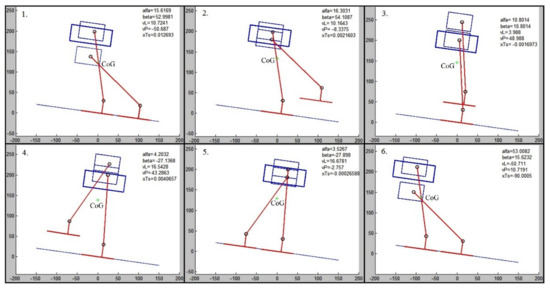
Figure 8.
Plotted robot configurations when walking on a pad with a slope of 8°. Legends: 1—the center of gravity of the robot is above the right foot; 2—the left linear actuator performs the upward stroke of the left foot; 3—the left ankle joint rotates to move the left foot forward and at the same time the right ankle joint balances the robot’s pose to the vertical position of the legs; the right linear actuator also works to keep the base at a constant height; 4—the left ankle joint transmits the left foot forward and at the same time the left linear actuator lowers the foot; the right linear actuator also lifts the base to keep it at a constant height. 5—the left foot is lowered to the ground; 6—both ankle joints rotate so that the center of gravity is transferred above the left foot and at the same time the height position of the base is compensated by the movement of both linear actuators.
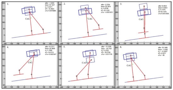
Figure 9.
Plotted configurations of the robot when walking on a pad with a slope of –8°. Legends: 1—the center of gravity of the robot is above the right foot; 2—the left linear actuator performs the upward stroke of the left foot; 3—the left ankle joint rotates to move the left foot forward and at the same time the right ankle joint balances the robot’s pose to the vertical position of the legs; the right linear actuator also works to keep the base at a constant height; 4—the left ankle joint transmits the left foot forward and at the same time the left linear actuator lowers the foot; the right linear actuator also lifts the base to keep it at a constant height. 5—the left foot is lowered to the ground; 6—both ankle joints rotate so that the center of gravity is transferred above the left foot and at the same time the height position of the base is compensated by the movement of both linear actuators.
7. Simulations of Robot Walking
For the implementation of all non-standard components, a transparent polycarbonate is chosen in order to achieve the minimum weight of the robot components at higher strength. This material is also used in the simulations. Steel is chosen for the rocker lever. In the simulations, batteries are also considered, which are located in the lowest position to lower the robot’s center of gravity.
The simulations are performed as co-simulations in SolidWorks Motion, Adams Multibody, and MATLAB environments. The non-standard components are made of polycarbonate and their weights are taken from the SolidWorks environment. Other components have factory-defined weights: Firgelli L12 the linear actuator weighs 56 g, the HS-645MG rotary actuator weighs 55 g, the HS-82MG rotary actuator weighs 19 g, and the Li-Pol 1600 mAh/11.1 V battery weighs 159 g (2 pieces are used).
The simulation is an experimental method in which the real system is replaced by a computer model. This model is subjected to experiments, from which the required information is subsequently obtained. To create advanced motion simulations of mechanisms, it is advantageous to use the SolidWorks Motion tool, which is built on Adams Multibody Dynamics Technology. This tool allows the calculation of dynamics considering inertial, reaction force, damping, and friction effects. From the recalculated results from the simulations of the created models, it is possible to easily plot the graphs of speed, acceleration, acting forces, and moments, or even the consumed power or the path of locomotion.
To create a step simulation, it is necessary to know the dependencies of the generalized coordinates α, β, vL, and vP, which represent the rotations or strokes of the servomotors. These are obtained using a program created in the MATLAB environment, which uses the equations derived in the chapter on robot stability. For proper functionality, the weights and positions of the centers of gravity of the individual parts of the walking robot are defined in the program. The input data for this program is a matrix containing the dependencies of foot positions xP and yP, the position of the robot’s center of gravity xT, the height of the robot’s base vZ, and the value of the inclination of the plane ϕ (Figure 10).
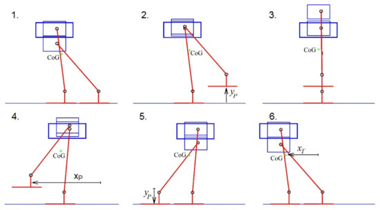
Figure 10.
Changes in the position of the foot and center of gravity of the robot during the step. Legends: 1—the center of gravity of the robot is above the right foot; 2—the left linear actuator performs the upward stroke of the left foot; 3—the left ankle joint rotates to move the left foot forward and at the same time the right ankle joint balances the robot’s pose to the vertical position of the legs; the right linear actuator also works to keep the base at a constant height; 4—the left ankle joint transmits the left foot forward and at the same time the left linear actuator lowers the foot; the right linear actuator also lifts the base to keep it at a constant height. 5—the left foot is lowered to the ground; 6—both ankle joints rotate so that the center of gravity is transferred above the left foot and at the same time the height position of the base is compensated by the movement of both linear actuators.
From the individual phases of the step according to (Figure 10), dependencies can be created and used as input data for the program to calculate the graphs of generalized coordinates, which ensure the static stability of the robot at each moment of walking (Figure 11).
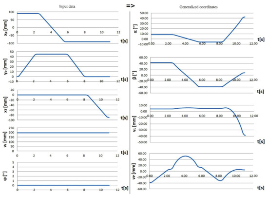
Figure 11.
Recalculation of generalized coordinates based on input data for horizontal plane walking.
First, the type of contact between the robot’s feet and the pad is defined and the direction of gravity is determined. Subsequently, the actuators are set using the motor function, where dependencies of generalized coordinates to the given motors are inserted via the data points option (Figure 12).
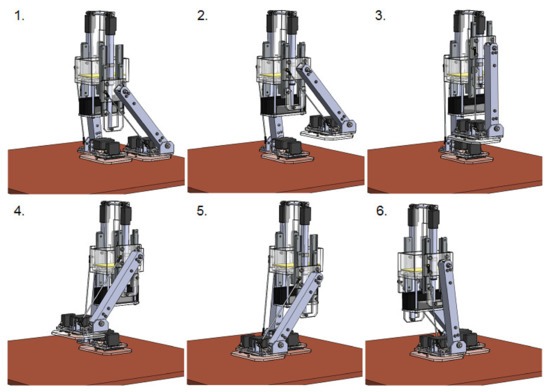
Figure 12.
Snapshot sequence from the created robot step simulation. Legends: 1—the center of gravity of the robot is above the right foot; 2—the left linear actuator performs the upward stroke of the left foot; 3—the left ankle joint rotates to move the left foot forward and at the same time the right ankle joint balances the robot’s pose to the vertical position of the legs; the right linear actuator also works to keep the base at a constant height; 4—the left ankle joint transmits the left foot forward and at the same time the left linear actuator lowers the foot; the right linear actuator also lifts the base to keep it at a constant height. 5—the left foot is lowered to the ground; 6—both ankle joints rotate so that the center of gravity is transferred above the left foot and at the same time the height position of the base is compensated by the movement of both linear actuators.
After recalculating the simulation, the following results can be displayed using the results and plots function (Figure 13):
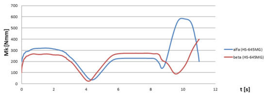
Figure 13.
Graph of rotational actuator torques.
The load moment graph for the HS-645MG rotary actuators is shown below.
The highest torque is reached within 9.95 s of 585 N·mm. From the catalog data from the manufacturer for the HS-645MG servomotors, the value of the maximum torque at the 6 V supply is obtained, which has a size of 9.6 kg·cm (i.e., 942 N·mm). By comparing these values, it can be stated that the actuator is suitable for the application.
A load graph for the Firgelli L12 linear actuators is shown in Figure 14.
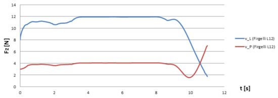
Figure 14.
Load graph of linear actuators.
It is possible to read from the graph that the greatest force acting on the linear servomotors reaches 12 N. The value of the maximum working load of the Firgelli L12 servomotor is stated in the catalogue data from the manufacturer, with a value of 24.5 N. Therefore, the use of this member in the robot design is satisfactory.
The position of the total center of gravity of the walking robot in the simulation is shown in Figure 15.
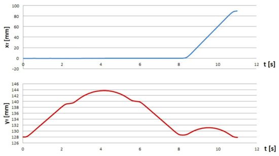
Figure 15.
Graph of the robot’s center of gravity position during the step.
The displayed graph of the xT value shows that the projection of the robot’s center of gravity during the step phase when the foot is crossed is located exactly in the middle above the foot, which is in contact with the pad. Thus, the projection is located as far as possible from the edge of the robot’s support base, meaning the highest possible degree of static stability is achieved. If the crossing phase ends, the center of gravity projection then moves over the other foot, ending the one-step cycle.
The changes in position of the robot’s base during the step are shown in Figure 16.
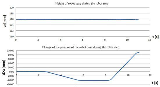
Figure 16.
Changes in position of the robot’s base during the step.
The height of the base of the robot (Figure 16) is kept constant during the step, and one of the requirements for the gait of the proposed robot is met. The second graph (Figure 16) shows that in the first stages of the step, the base of the robot performs a slight backward movement, thereby balancing the forward movement of the robot’s foot. After this movement, the base of the robot is then moved forward to the desired position, which results from the determined step length.
7.1. Robot Rotation Simulation
The rotation simulation is performed in order to verify the actuator design in changing the walking direction of the robot. The rotation of the robot by an angle of 30° within 2 s is then simulated (Figure 17 and Figure 18).
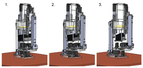
Figure 17.
Snapshot sequence from the robot rotation simulation. Legends: 1—both legs of the robot are in a vertical plane and at the same time the robot is standing on the right foot; 2—the rotary actuator rotates the rotary pad by the required angle of rotation; 3—the robot is in the target position of the angle of rotation and is ready to lower down the left foot and transfer the center of gravity of the robot to it and then raise the right foot and rotate the right rotary actuator to return the right rotary pad to its original position.
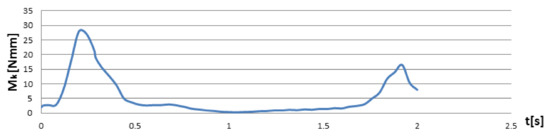
Figure 18.
Torque graph for the HS-82MG servomotor.
According to the values in the catalogue sheet, the HS-82MG rotary actuator can reach a maximum torque of 3.4 kg·cm (333.5 N·mm) at a supply voltage of 6 V. Since the largest torque value required to rotate the robot is 28.5 N·mm, the use of this servomotor is satisfactory.
7.2. Simulation of a Robot Step on an Inclined Plane
To simulate walking on an inclined plane, a coefficient of friction is selected for a rubber–dry concrete material pair with a static coefficient of friction value (0.8). Experiments are performed to determine the static coefficient of friction [42].
In a similar way that the step-by-plane simulation is created, the step-by-plane simulation is created. The calculation in the MATLAB environment is used again, with the help of which the graphs of generalized coordinates are calculated (Figure 19).
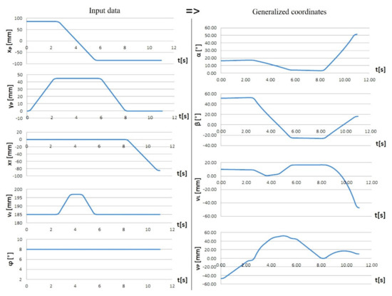
Figure 19.
Recalculation of generalized coordinates based on input data for slope 8°.
In the simulations, a slope angle of 8° is considered (Figure 19). As can be seen in the graphs, when walking on an inclined plane, there are greater demands on the range of linear servomotors, meaning this fact has to be compensated for using a slight change in the height of the base (Figure 19). From these results, an image sequence of the robot’s movement along the inclined plane is subsequently generated (Figure 20).
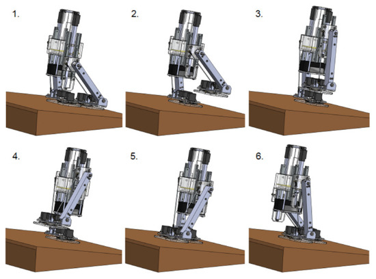
Figure 20.
Snapshots sequence from a step simulation of a pad with an 8° uphill slope. Legends: 1—the center of gravity of the robot is above the right foot; 2—the left linear actuator performs the upward stroke of the left foot; 3—the left ankle joint rotates to move the left foot forward and at the same time the right ankle joint balances the robot’s pose to the vertical position of the legs; the right linear actuator also works to keep the base at a constant height; 4—the left ankle joint transmits the left foot forward and at the same time the left linear actuator lowers the foot; the right linear actuator also lifts the base to keep it at a constant height. 5—the left foot is lowered to the ground; 6—both ankle joints rotate so that the center of gravity is transferred above the left foot and at the same time the height position of the base is compensated by the movement of both linear actuators.
8. Discussion and Plans for Further Research
In this work, a biped walking robot (Figure 21) was designed based on a concept that envisaged the use of six actuators. Two rotary and two linear servomotors were designed to allow the robot to walk and the other two rotary actuators were used to change the direction of movement. The concept was based on a parallelogram that ensured a constant parallel relationship between the base and the robot’s feet.
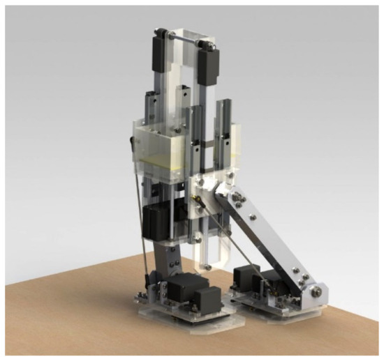
Figure 21.
Designed biped robot with a vertically stabilized base.
The direct kinematics task was solved with the help of the created kinematic model of the robot, where the main points of the chain and the centers of gravity of the individual parts were assigned local coordinate systems. A possible additional device in the robot’s base (manipulator, sensors, etc.) could also be included in the proposed kinematic chain. The direct kinematics problem was solved by considering the inclination of the plane in the direction of the robot’s gait. Subsequently, the inverse kinematics equations were derived using the vector inverse transform method. The obtained data were used as the basis for the static walking simulations on straight and inclined pads, confirming the ability of the concept to overcome a rise or fall during tilting in the direction of walking. The stable configuration of the robot during the individual phases of the step was recalculated using programs created in the MATLAB environment, which were also used to recalculate the generalized coordinates needed to create a walking simulation. In the SolidWorks Motion environment, a step on a flat surface, a step on a surface with an 8° uphill slope, and the rotation of the robot were simulated.
The results from the given simulations confirmed the fulfillment of the required criteria, such as maintaining a constant height for the robot’s base and allowing adjustments of the height and the minimum inclinations, which significantly improved the conditions when adding additional equipment to the robot’s base. The simulations also verified that the actuators used are suitable for this application.
The adaptability of the presented model will depend not only on the structural concept of the model but also on the control method used. These problems will be solved in the near future, also directly on the experimental functional prototype. The aim of this work was first to use simulations to evaluate the usability and viability of this robot concept. Control issues will largely depend on the control method used and will be addressed in a separate paper.
The energy efficiency of this principle was not solved in this work, but the simulations probably show the courses of moments and speeds of individual actuators, and on the basis of this information it is possible to assess the energy efficiency of this robot. An energy efficiency test will be determined experimentally on a functional prototype, which will be the subject of further research.
The designed robot ensures the function of the gait itself and also allows the direction of movement to be changed. Therefore, the possibilities for further development of the robot are very wide and depend mainly on its future use. The submitted proposals for further research and development are listed below:
- Implement a system for measuring the inclination of a plane consisting of an inertial measurement unit sensor containing gyroscopes and accelerometers. In this way, it will be possible to detect the inclination of the robot’s base, which will be identical to the inclination of the plane thanks to the parallelogram, and to use this detected information to automatically correct the stability of the robot on an inclined plane [43];
- Use sensor equipment to move and navigate the robot in an unknown environment. Obstacle sensors may include an anti-collision ultrasonic sensor and an optical sensor. The determination of the orientation and position in space can be achieved by recording the distance traveled by the accelerometer. Alternatively, simultaneous mapping of the environment in which the robot is moving can be achieved [44,45];
- Complete the design with two more degrees of freedom in the foot, which will allow walking on a plane inclined perpendicular to the walking direction;
- Since the designed robot has the precondition to overcome height obstacles, it would be appropriate to supplement it with a system for measuring the sizes of such obstacles and to design a walking algorithm to overcome them;
- Place an additional device on the robot’s base to perform additional functions, e.g., an object manipulator [46,47,48,49,50] or camera device. The platform has very advantageous features for this purpose, as it experiences minimal tilting during walking and maintains a constant height;
- Equip the robot with a teleoperator system for control via a remote-controlled panel also with environmentally focused systems [51,52,53,54].
- Deal with the issue of dynamic stability when walking, which will allow faster and smoother movement of the robot.
9. Conclusions
The basic problem with conventional biped robots is that when the base moves, the robot performs a rocking spatial movement to the side, meaning the placement of anti-collision and environmental mapping sensors can be quite problematic. Additionally, if the robot is equipped with a handling device, it will be hard to grip objects if the robot moves. These sideways oscillations can also cause problems when moving objects.
In this work, however, a biped robot was designed with vertical stabilization of the robot’s base and minimization of its sideways oscillations. Although the proposed concept no longer has the attributes of a humanoid robot, as a linear coupling with a linear actuator was used, thanks to this modification the stabilizing effect of the base in the vertical direction was achieved.
The main contribution of this work is the creation of a two-legged robot concept, which has a vertically stabilized base with a minimum number of actuators. In addition, this design also handles walking on inclined planes and in rugged terrain with obstacles.
This robot uses 6 actuators, which gives good preconditions for energy balance compared to purely articulated bipedal robots. In addition, the linear actuator used is self-locking, so no additional energy is required to brake or keep it in a stable position.
The actuator self-locking means that it does not need to use the brake to keep it in position when the power is off. Alternatively, it is necessary to integrate either a mechanical brake or an electric brake into the drive, especially for those actuators that do not have a self-locking phenomenon. Self-locking is influenced by the gear ratio and the used gear principle, clearances, friction, and other factors. Some actuator manufacturers also include self-locking force values in the datasheet, or it is possible to identify these values experimentally. It is, therefore, a good idea to consider this self-locking system when designing a robot. Usually, robots have to use extra energy to brake their actuators to maintain their position.
Special attention in the design was focused on the position of the robot’s center of gravity and its stability in motion, which is very often a neglected aspect in the design of this type of robot.
Since it is a robot that moves with the help of legs, there is also the possibility to move it in rugged terrain, where other types of mobile robots could have problems overcoming obstacles.
Due to the stated features of this concept, this proposal has several benefits and is suitable for use in several areas. This concept can be used for the construction of a mechatronic assistant, which would help people during normal work at home, in industry, or in patient care, where it would also allow the transport of patients. For application as a mechatronic assistant, it is still necessary to supplement it with a handling structure and other equipment. Such an assistant could help people to carry heavy things while overcoming the obstacles common to an urban environment. A big problem for physically handicapped people is also their movement by means of wheelchairs, so this concept, with its suitable size, is a potential concept for use in the construction of a two-legged vehicle for people with disabilities. This two-legged concept is unique in that compared to wheeled concepts, it is able to walk on sloping terrain, even with potential obstacles, of which there are a huge number in urban areas, meaning these people with disabilities would be able to use this innovative concept for completely independent movement. The independence of these people is important not only physically but also mentally, as in many situations they require outside help. This concept of a two-legged transport device would, thus, bring a new dimension to their lives. In this regard, we consider this work to be very important and necessary.
Author Contributions
Data curation, Ľ.M.; funding acquisition, T.K. and M.V. (Martin Varga); investigation, R.R.; methodology, M.V. (Marek Vagaš); resources, J.S.; software, R.J.; supervision, I.V.; validation, M.S.; visualization, M.S.; writing—original draft, P.M.; writing—review and editing, P.T. All authors have read and agreed to the published version of the manuscript.
Funding
This research was funded by Slovak Grant Agency VEGA 1/0201/21 and VEGA 1/0436/22.
Institutional Review Board Statement
Not applicable.
Informed Consent Statement
Not applicable.
Data Availability Statement
Not applicable.
Acknowledgments
The authors would like to thank the Slovak Grant Agency VEGA 1/0201/21 and VEGA 1/0436/22.
Conflicts of Interest
The authors declare no conflict of interest. The funders had no role in the design of the study; in the collection, analyses, or interpretation of data; in the writing of the manuscript; or in the decision to publish the results.
References
- Kahraman, C.; Deveci, M.; Boltürk, E.; Türk, S. Fuzzy controlled humanoid robots: A literature review. Robot. Auton. Syst. 2020, 134, 103643. [Google Scholar] [CrossRef]
- Brooks, R.A.; Breazeal, C.; Marjanović, M.; Scassellati, B.; Williamson, M.M. The Cog Project: Building a Humanoid Robot. In Computation for Metaphors, Analogy, and Agents. CMAA 1998; Nehaniv, C.L., Ed.; Lecture Notes in Computer Science; Springer: Berlin/Heidelberg, Germany, 1998; Volume 1562. [Google Scholar] [CrossRef]
- Wong, C.C.; Cheng, C.T.; Huang, K.H.; Yang, Y.T. Fuzzy control of humanoid robot for obstacle avoidance. Int. J. Fuzzy Syst. 2008, 10, 1–10. [Google Scholar] [CrossRef]
- Sakagami, Y.; Watanabe, R.; Aoyama, C.; Matsunaga, S.; Higaki, N.; Fujimura, K. The intelligent ASIMO: System overview and integration. In Proceedings of the IEEE/RSJ International Conference on Intelligent Robots and Systems, Lausanne, Switzerland, 30 September–4 October 2002; IEEE: Piscataway, NJ, USA, 2002; Volume 3, pp. 2478–2483. [Google Scholar] [CrossRef]
- Hirai, K.; Hirose, M.; Haikawa, Y.; Takenaka, T. The development of honda humanoid robot. In Proceedings of the 1998 IEEE International Conference on Robotics and Automation (Cat. No.98CH36146), Leuven, Belgium, 16–20 May 1998; Volume 2, pp. 1321–1326. [Google Scholar] [CrossRef]
- Nishiwaki, K.; Sugihara, T.; Kagami, S.; Kanehiro, F.; Inaba, M.; Inoue, H. Design and development of research platform for perception-action integration in humanoid robot: H6. In Proceedings of the 2000 IEEE/RSJ International Conference on Intelligent Robots and Systems (IROS 2000) (Cat. No.00CH37113), Takamatsu, Japan, 31 October–5 November 2000; Volume 3, pp. 1559–1564. [Google Scholar] [CrossRef]
- Oh, J.H.; Hanson, D.; Kim, W.S.; Han, Y.; Kim, J.Y.; Park, I.W. Design of android type humanoid robot Albert HUBO. In Proceedings of the 2006 IEEE/RSJ International Conference on Intelligent Robots and Systems, Beijing, China, 9–15 October 2006; pp. 1428–1433. [Google Scholar] [CrossRef]
- Park, H.Y.; Kim, J.H.; Yamamoto, K. A New Stability Framework for Trajectory Tracking Control of Biped Walking Robots. IEEE Trans. Ind. Inform. 2022, 1–11. [Google Scholar] [CrossRef]
- Chen, H.; Chen, X.; Yu, Z.; Dong, C.; Li, Q.; Zhang, R.; Huang, Q. A Swing-foot Trajectory Generation Method For Biped Walking. In Proceedings of the 2021 6th IEEE International Conference on Advanced Robotics and Mechatronics (ICARM), Chongqing, China, 3–5 July 2021; pp. 841–845. [Google Scholar] [CrossRef]
- Rosa, N.; Lynch, K.M. A Topological Approach to Gait Generation for Biped Robots. IEEE Trans. Robot. 2021, 38, 699–718. [Google Scholar] [CrossRef]
- Gao, Z.; Chen, X.; Yu, Z.; Zhu, M.; Zhang, R.; Fu, Z.; Li, C.; Li, Q.; Han, L.; Huang, Q. Autonomous Navigation with Human Observation for a Biped Robot. In Proceedings of the 2021 IEEE International Conference on Unmanned Systems (ICUS), Beijing, China, 22–24 October 2021; pp. 780–785. [Google Scholar] [CrossRef]
- Zhu, X.; Wang, L.; Yu, Z.; Chen, X.; Han, L. Motion Control for Underactuated Robots Adaptable to Uneven Terrain by Decomposing Body Balance and Velocity Tracking. In Proceedings of the 2021 6th IEEE International Conference on Advanced Robotics and Mechatronics (ICARM), Chongqing, China, 3–5 July 2021; pp. 729–734. [Google Scholar] [CrossRef]
- Fevre, M.; Lin, H.; Schmiedeler, J.P. Stability and Gait Switching of Underactuated Biped Walkers. In Proceedings of the 2019 IEEE/RSJ International Conference on Intelligent Robots and Systems (IROS), Macau, China, 3–8 November 2019; pp. 2279–2285. [Google Scholar] [CrossRef]
- Sobirin, M.; Hindersah, H. Stability Control for Bipedal Robot in Standing and Walking using Fuzzy Logic Controller. In Proceedings of the 2021 IEEE International Conference on Industry 4.0, Artificial Intelligence, and Communications Technology (IAICT), Bali, Indonesia, 7–8 July 2021; pp. 1–7. [Google Scholar] [CrossRef]
- Yu, J.; Li, C.; Gong, D.; Zuo, G.; Wang, Y. Walking Simulation of Biped Robot on Inclined Plane Based on Gait Recognition. In Proceedings of the 2020 IEEE International Conference on Real-time Computing and Robotics (RCAR), Hokkaido, Japan, 28–29 September 2020; pp. 256–261. [Google Scholar] [CrossRef]
- Safartoobi, M.; Dardel, M.; Daniali, H.M. Gait cycles of passive walking biped robot model with flexible legs. Mech. Mach. Theory 2021, 159, 104292. [Google Scholar] [CrossRef]
- Shibata, T.; Wada, K. Robot therapy: A new approach for mental healthcare of the elderly—A mini-review. Gerontology 2011, 57, 378–386. [Google Scholar] [CrossRef]
- Mende, M.; Scott, M.L.; Van Doorn, J.; Grewal, D.; Shanks, I. Service Robots Rising: How Humanoid Robots Influence Service Experiences and Elicit Compensatory Consumer Responses. J. Mark. Res. 2019, 56, 535–556. [Google Scholar] [CrossRef]
- Huang, S.; Tanioka, T.; Locsin, R.; Parker, M.; Masory, O. Functions of a caring robot in nursing. In Proceedings of the 2011 7th International Conference on Natural Language Processing and Knowledge Engineering, Tokushima, Japan, 27–29 November 2011; pp. 425–429. [Google Scholar] [CrossRef]
- Jyh-Hwa, T.; Kuo, L.S. The development of the restaurant service mobile robot with a laser positioning system. In Proceedings of the 2008 27th Chinese Control Conference, Kunming, China, 16–18 July 2008; pp. 662–666. [Google Scholar] [CrossRef]
- Collins, S.H.; Wiggin, M.B.; Sawicki, G.S. Reducing the energy cost of human walking using an unpowered exoskeleton. Nature 2015, 522, 212–215. [Google Scholar] [CrossRef]
- Lan, C.W.; Lin, S.S.; Ku, C.T.; Chen, B.S.; Lo, M.F.; Chien, M.C. Design and Development of a Biped Robot for a Knee Exoskeleton Analysis. In Proceedings of the 2021 International Symposium on Intelligent Signal Processing and Communication Systems (ISPACS), Hualien, Taiwan, 16–19 November 2021; pp. 1–2. [Google Scholar] [CrossRef]
- Jatsun, S.; Yatsun, A.; Savin, S.; Postolnyi, A. Approach to motion control of an exoskeleton in “verticalization-to-walking” regime utilizing pressure sensors. In Proceedings of the 2016 IEEE International Conference on Cyber Technology in Automation, Control, and Intelligent Systems (CYBER), Chengdu, China, 19–22 June 2016; pp. 452–456. [Google Scholar] [CrossRef]
- Lv, G.; Lin, J.; Gregg, R.D. Trajectory-Free Control of Lower-Limb Exoskeletons Through Underactuated Total Energy Shaping. IEEE Access 2021, 9, 95427–95443. [Google Scholar] [CrossRef]
- Jackson, S.; Ellis, L.; Lui, C.; Molloy, P.; Paterson, K.; Chandrapal, M.; Chen, X.Q. Development of an active powered biped lower limb exoskeleton. In Proceedings of the 2014 IEEE International Conference on Automation Science and Engineering (CASE), Taipei, Taiwan, 18–22 August 2014; pp. 990–995. [Google Scholar] [CrossRef]
- Grimmer, M.; Holgate, M.; Holgate, R.; Boehler, A.; Ward, J.; Hollander, K.; Sugar, T.; Seyfarth, A. A powered prosthetic ankle joint for walking and running. Biomed. Eng. Online 2016, 15, 286. [Google Scholar] [CrossRef]
- Rashid, A.; Mahmood, A. Development and LQR Control of Prosthetic Leg Prototype for Human Gait. In Proceedings of the 2019 International Conference on Electrical, Communication, and Computer Engineering (ICECCE), Swat, Pakistan, 24–25 July 2019; pp. 1–5. [Google Scholar] [CrossRef]
- Yu, J.; Hooks, J.; Zhang, X.; Sung Ahn, M.; Hong, D. A Proprioceptive, Force-Controlled, Non-Anthropomorphic Biped for Dynamic Locomotion. In Proceedings of the 2018 IEEE-RAS 18th International Conference on Humanoid Robots (Humanoids), Beijing, China, 6–9 November 2018; pp. 1–9. [Google Scholar] [CrossRef]
- Ahn, M.S.; Hong, D. Dynamic, Robust Locomotion for a Non-Anthropomorphic Biped. In Proceedings of the 2020 17th International Conference on Ubiquitous Robots (UR), Kyoto, Japan, 22–26 June 2020; pp. 185–191. [Google Scholar] [CrossRef]
- Mikhalkov, N.; Prutskiy, A.; Sechenev, S.; Kazakov, D.; Simulin, A.; Sokolov, D.; Ryadchikov, I. Gyrubot: Nonanthropomorphic stabilization for a biped. In Proceedings of the 2021 IEEE International Conference on Robotics and Automation (ICRA), Xi’an, China, 30 May–5 June 2021; pp. 4976–4982. [Google Scholar] [CrossRef]
- Fierro, J.E.; Pamanes, J.A.; Aquino, J.A.; Ollervides, E.J. Analysis of a Humanoid Robot Walking in an Arbitrary Direction on an Sloping Surface. In Proceedings of the 2021 XXIII Robotics Mexican Congress (ComRob), Tijuana, Mexico, 27–29 October 2021; pp. 56–62. [Google Scholar] [CrossRef]
- Yang, L.; Lai, G.; Chen, Y.; Guo, Z. Online Control for Biped Robot with Incremental Learning Mechanism. Appl. Sci. 2021, 11, 8599. [Google Scholar] [CrossRef]
- Lisitano, D.; Bonisoli, E.; Recchiuto, C.; Muscolo, G. Dynamic Balance of the Head in a Flexible Legged Robot for Efficient Biped Locomotion. Appl. Sci. 2021, 11, 2945. [Google Scholar] [CrossRef]
- Li, L.; Xie, Z.; Luo, X.; Li, J. Effects of Torso Pitch Motion on Energy Efficiency of Biped Robot Walking. Appl. Sci. 2021, 11, 2342. [Google Scholar] [CrossRef]
- Liu, C.; Gao, J.; Tian, D.; Zhang, X.; Liu, H.; Meng, L. A Disturbance Rejection Control Method Based on Deep Reinforcement Learning for a Biped Robot. Appl. Sci. 2021, 11, 1587. [Google Scholar] [CrossRef]
- Zhang, J.; Yuan, Z.; Dong, S.; Sadiq, M.; Zhang, F.; Li, J. Structural Design and Kinematics Simulation of Hydraulic Biped Robot. Appl. Sci. 2020, 10, 6377. [Google Scholar] [CrossRef]
- Russo, M.; Ceccarelli, M.; Cafolla, D. Kinematic Modelling and Motion Analysis of a Humanoid Torso Mechanism. Appl. Sci. 2021, 11, 2607. [Google Scholar] [CrossRef]
- Mikolajczyk, T.; Borboni, A.; Kong, X.W.; Malinowski, T.; Olaru, A. 3D Printed Biped Walking Robot. In Applied Mechanics and Materials; Trans Tech Publications Ltd.: Zurich, Switzerland, 2015; Volume 772, pp. 477–481. [Google Scholar] [CrossRef]
- Chevallereau, C.; Razavi, H.; Six, D.; Aoustin, Y.; Grizzle, J. Self-synchronization and self-stabilization of 3D bipedal walking gaits. Robot. Auton. Syst. 2018, 100, 43–60. [Google Scholar] [CrossRef]
- Formalsky, A.; Yannick, A. Biped without Feet in Single Support: Stabilization of the Vertical Posture with Internal Torques. In Mobile Robots: Towards New Applications [Internet]; Lazinica, A., Ed.; IntechOpen: London, UK, 2006; Available online: https://www.intechopen.com/chapters/47 (accessed on 3 April 2022).
- Vařeka, I. Postural stability (part 1). Terminology and biomechanical principles. Rehabil. Phys. Med. 2002, 9, 115–121. [Google Scholar]
- Kelemenová, T.; Dovica, M.; Božek, P.; Koláriková, I.; Benedik, O.; Virgala, I.; Prada, E.; Miková, L.; Kot, T.; Kelemen, M. Specific Problems in Measurement of Coefficient of Friction Using Variable Incidence Tribometer. Symmetry 2020, 12, 1235. [Google Scholar] [CrossRef]
- Pastor, M.; Kelemenová, T.; Kelemen, M.; Miková, L.; Baláž, R. Declination Angle Gage for Tilt Measurement Sensors. Procedia Eng. 2012, 48, 549–556. [Google Scholar] [CrossRef]
- Babinec, A.; Duchoň, F.; Dekan, M.; Pásztó, P.; Kelemen, M. VFH*TDT (VFH* with Time Dependent Tree): A new laser rangefinder based obstacle avoidance method designed for environment with non-static obstacles. Robot. Auton. Syst. 2014, 62, 1098–1115. [Google Scholar] [CrossRef]
- Oščádal, P.; Heczko, D.; Vysocký, A.; Mlotek, J.; Novák, P.; Virgala, I.; Sukop, M.; Bobovský, Z. Improved Pose Estimation of Aruco Tags Using a Novel 3D Placement Strategy. Sensors 2020, 20, 4825. [Google Scholar] [CrossRef] [PubMed]
- Kelemen, M.; Virgala, I.; Lipták, T.; Miková, L.; Filakovský, F.; Bulej, V. A Novel Approach for a Inverse Kinematics Solution of a Redundant Manipulator. Appl. Sci. 2018, 8, 2229. [Google Scholar] [CrossRef]
- Virgala, I.; Kelemen, M.; Varga, M.; Kuryło, P. Analyzing, Modeling and Simulation of Humanoid Robot Hand Motion. Procedia Eng. 2014, 96, 489–499. [Google Scholar] [CrossRef]
- Virgala, I.; Gmiterko, A.; Kelemen, M.; Miková, L.; Varga, M. Inverse Kinematic Model of Humanoid Robot Hand. Appl. Mech. Mater. 2014, 611, 75–82. [Google Scholar] [CrossRef]
- Miková, L.; Kelemen, M.; Virgala, I.; Michna, M. Simulation Model of Manipulator for Model Based Design. Appl. Mech. Mater. 2014, 611, 175–182. [Google Scholar] [CrossRef]
- Virgala, I.; Gmiterko, A.; Surovec, R.; Vacková, M.; Prada, E.; Kenderová, M. Manipulator End-Effector Position Control. Procedia Eng. 2012, 48, 684–692. [Google Scholar] [CrossRef][Green Version]
- Kelemen, M.; Kelemenová, T.; Virgala, I.; Miková, L.; Lipták, T. Rapid Control Prototyping of Embedded Systems Based on Microcontroller. Procedia Eng. 2014, 96, 215–220. [Google Scholar] [CrossRef]
- Piňosová, M.; Andrejiová, M.; Lumnitzer, E. Synergistic Effect of Risk Factor and Work Environmental Quality. Qual.-Access Success 2018, 19, 154–159. [Google Scholar]
- Lumnitzer, E.; Liptai, P.; Drahoš, R. Measurement and Assessment of Pulsed Magnetic Fields in the Working Environment. In Proceeding of the 8th International Scientific Symposium on Electrical Power Enginering (Elektroenergetika 2015), Stara Lesna, Slovakia, 16–18 September 2015; pp. 331–333. [Google Scholar]
- Puškár, M.; Jahnátek, A.; Kádárová, J.; Šoltésová, M.; Kovanič, Ľ.; Krivosudská, J. Environmental study focused on the suitability of vehicle certifications using the new European driving cycle (NEDC) with regard to the affair “dieselgate” and the risks of NOx emissions in urban destinations. Air Qual. Atmos. Health 2018, 12, 251–257. [Google Scholar] [CrossRef]
Publisher’s Note: MDPI stays neutral with regard to jurisdictional claims in published maps and institutional affiliations. |
© 2022 by the authors. Licensee MDPI, Basel, Switzerland. This article is an open access article distributed under the terms and conditions of the Creative Commons Attribution (CC BY) license (https://creativecommons.org/licenses/by/4.0/).