On the Applicability of Approximate Rolling and Sliding Contact Algorithms in Anisothermal Problems with Thermal Softening

Abstract

The residual stress approximation methods formulated by McDowell and Moyar, Jiang and Sehitoglu, and McDowell for rolling and sliding contact problems are reconsidered in the context of single anisothermal loading cycles and isotropic hardening. A consistent extention to incorporate thermal softening is developed and the generalized thermoelastoplastic algorithms are cast into a proper predictor–corrector formulation. Detailed explicit and implicit numerical integration strategies are presented and validated using specifically designed finite element models that conform to the underlying mechanical assumptions. Then, the applicability of the approximate algorithms to anisothermal problems with isotropic hardening and thermal softening is analyzed by assuming a rate-independent Johnson–Cook-type yield stress model and by comparing the obtained transient and residual stresses to results from full-scale finite element half-space models under varying loading and strain-hardening intensities. An in-depth, comparative discussion on the adequacy of the algorithms in conjunction with the justification of their respective mechanical simplifications follows. Sufficiently strong strain hardening is found to be a prerequisite for accurate predictions, and Jiang and Sehitoglu’s approach is deemed to be preferable for the considered type of problem. The conclusions drawn from the investigations are discussed in the context of common applications with particular emphasis on manufacturing process modeling and the corresponding guidelines are proposed for such use cases.

1. Introduction

Residual stresses often are an important factor for the fatigue life of components when dynamic thermomechanical loads have to be endured during service. Fatigue failure frequently originates at the component surface due to its roughness and exposition to extremal loads (promoted e.g., by notches or bending and torsion) as well as to other possibly adverse environmental conditions. Hence, it is important to be aware in particular of surface and near-surface residual stresses that often arise during manufacturing. Machining, as an important example, is widely applied for the surface finishing of metal components, and thus, machining-induced residual stresses have been studied intensively via analytical, numerical and experimental means [1,2,3]. Due to the advancement of computational capabilities, the finite element (FE) method has been established as the standard tool for such investigations nowadays. Nevertheless, more efficient approximate approaches are still of interest in special applications. As an extreme example, FE approaches are prohibitively expensive if real-time capability is desired e.g., for model-based manufacturing process control [4]. Given such circumstances, one might resort to simpler, semi-analytical modeling strategies. In many cases, these revolve around modeling the actual processing by considering elastoplastic half-spaces subjected to transient surface loads, which must be appropriately abstracted from the underlying physical processes.

Pioneering work on semi-analytical residual stress prediction schemes based on such modeling has been done in the context of wheel–rail systems. Among the earliest is the influential paper of Merwin and Johnson [5], who propose to incrementally and approximately solve the elastoplastic problem for a fixed set of material points along the depth while the surface loads pass by. Their key simplification is the assumption that the transient strains during this procedure may be equated to the corresponding elastic solution, which enables an uncoupled and thus efficient treatment of each considered discrete depth. To satisfy the conditions on the stresses and strains in the stationary state implied by the boundary conditions and homogeneity, they apply a subsequent elastoplastic relaxation procedure. Later, McDowell and Moyar [6] and Jiang and Sehitoglu [7] build upon the core ideas of Merwin and Johnson [5] to formulate similar algorithms with altered assumptions on the transient stresses and strains during the loading pass. McDowell [8] found their approaches to work reasonably well in different parameter ranges within isothermal rolling and sliding contact problems under kinematic hardening, and thus, he proposed to combine them via blending the respective differential equations in a heuristic way.

One of the first applications of the above approximate algorithms in the context of manufacturing is the work of Jacobus et al. [1], who employ the method of Merwin and Johnson [5] and generalize it to account for thermal strains. Using experimentally determined displacement fields to define the transient strains and a finite-difference scheme for the heat conduction problem, they predicted residual stresses induced by orthogonal and oblique cutting operations. Ulutan et al. [9] and Liang and Su [10] later published similar applications using the algorithms of Jiang and Sehitoglu [7] and McDowell [8], respectively, while applying analytic cutting force models to estimate the surface loads’ magnitudes. Since then, a multitude of methodologically rather similar studies have been carried out for various manufacturing processes such as turning [11,12], milling [13,14,15], or additive manufacturing [16,17], which differ w.r.t. the surface load modeling but all rely on the same mechanical baseline assumptions and the algorithms of Jiang and Sehitoglu [7] or McDowell [8] to attempt estimating residual stresses depth profiles.

In the scope of such applications, these approximate algorithms have been applied to problems and constitutive models well away from their original purposes in the modelling of elastoplastic rolling and sliding contact. Specifically, only a single pass of the surface loads, isotropic hardening, thermal stresses and possibly temperature-dependent constitutive parameters are usually considered as opposed to the focus on multiple loading cycles, kinematic hardening, and isothermal problems prevalent in rolling contact research. However, systematic and thorough analysis of the adequacy of the mentioned approximate algorithms on more theoretical grounds seems to be mostly limited to these latter circumstances of rolling contact; see e.g., the works of Bhargava et al. [18,19] and Xu and Jiang [20] as well as [7,8].

The present paper aims to close this knowledge gap by analyzing the applicability of the approximate algorithms [6,7,8] under conditions more relevant to manufacturing applications. Specifically, we consider single-pass thermomechanical surface loads and isotropic hardening (according to a Johnson–Cook-type yield stress model)—while investigating the quality of the predicted residual stresses using reference solutions from appropriate FE models. This enables an in-depth discussion of the approximate algorithms’ accuracy in conjunction with their underlying additional simplifications regarding certain transient stress and strain components. Furthermore, we generalize and reformulate the algorithms to account for thermal softening in a consistent way, which is necessary in case of temperature-dependent yield strength but has not been done previously. In doing so, we cast the algorithms’ treatment of elastoplastic increments into a proper predictor–corrector form and provide detailed implementation-ready numerical schemes for both explicit and implicit solutions of the corrector step. The implicit scheme is deemed particularly useful when the evaluation of the elastic input solution on very fine grids comes at a computational cost that is non-negligible to the application, e.g., when real-time predictions are needed [4]. In such cases, larger step sizes might be preferable over the additional effort introduced by an implicit integration method.

The structure of the paper is as follows: In Section 2, the thermomechanical half-space problem under consideration is stated, the residual stress approximation algorithms [6,7,8] are reformulated, and their numerical solution is detailed. Next, we describe the FE models, which we later on use to validate and benchmark our implementations of said algorithms, in Section 4, where we also discuss their properties and assumptions in the context of our numerical studies. A boarder discussion follows in Section 5, where we shift the focus toward applications and the corresponding literature. Finally, conclusions on the applicability of the considered approximate methods are drawn in Section 6.

2. Thermoelastoplastic Approximate Algorithms

The purpose of this section is two-fold. First, we reformulate the methods of McDowell and Moyar [6] and of Jiang and Sehitoglu [7]—abbreviated by “MM” and “JS”, respectively—for anisothermal problems in which isotropic strain hardening is accompanied by thermal softening. Then, algorithms and guidelines for the numerical solution of the arising differential equation systems will be provided.

The thermomechanical problem under consideration is visualized in Figure 1. It consists of a thermoelastoplastic half-space under plane-strain conditions which is loaded by a moving heat flux distribution as well as by distributed normal and tangential surface tractions. The $\xi$-$\eta$-system (we may drop the out-of-plane coordinates $\zeta$ and z indicated in Figure 1 in most of our discussion, since the assumption of plane-strain precludes any gradients in these coordinate directions), within which the distributions are stationary, moves at constant velocity v in the $\xi$-direction w.r.t. the x-y-system that is fixed to the material points of the half-space. In this setting, the material derivative of any tensor field F on the half-space reduces to its convective part within the $\xi$-$\eta$-system, i.e.,

$$\begin{array}{c}\hfill \dot{F}=\frac{\mathrm{D}F}{\mathrm{D}t}=-\frac{\partial F}{\partial \xi }v,\end{array}$$

(1)

where $\mathrm{D}(•)/\mathrm{D}t$ denotes the material derivative, so that temporal changes of state in the material x-y-system correspond to spatial changes in the $\xi$-$\eta$-system, and our whole discussion can be continued in the latter coordinate system.

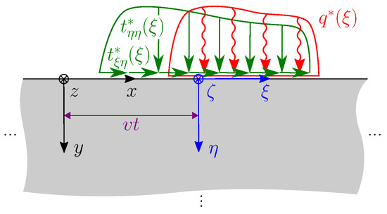
Figure 1. Half-space loaded by a distributed surface heat flux $q^{*}\left(\xi \right)$ and normal and tangential surface tractions $t_{\eta \eta }^{*}\left(\xi \right)$, $t_{\xi \eta }^{*}\left(\xi \right)$. Assuming a quasi-stationary problem, the distributions are constant in time in the $\xi$-$\eta$-$\zeta$-system that moves at constant velocity v in the $\xi$-direction w.r.t. the material coordinate system x-y-z. The coordinate axes pointing into the plane are denoted by $\zeta$ and z, respectively. The assumption of plane-strain implies zero total normal strain along these axes, i.e., ${\epsilon }_{\zeta \zeta }={\epsilon }_{zz}=0$.

Assume now that the quasi-stationary solution of the thermoelastic half-space problem is known at least on (a discretization of) a sufficiently large domain ${\Omega }^{*}$ in the $\xi$-$\eta$-plane which contains the support of the load distributions. By sufficiently large, we imply that the stresses and temperature on the complement set of ${\Omega }^{*}$ will not suffice to cause or sustain plastic flow of a passing material point, which may be estimated using the chosen yield condition (e.g., Equation (2)) under the assumption of no prior strain hardening and of decaying stresses and temperature beyond the vicinity of the loads. Then, the underlying idea of the MM and JS algorithms is to approximate the thermoelastoplastic response of a material point passing through ${\Omega }^{*}$ in a fixed depth $\eta$ by subjecting it to specific in-plane components of the stress tensor ${\sigma }_{ij}^{*}$ as well as the temperature $T^{*}$ from the thermoelastic solution while solving for the remaining stress components by means of classical von Mises plasticity and—in case of the MM algorithm—using an additional kinematic constraint. We will expand on this in detail and provide the full algorithms in Section 2.2, but before, we shall state the equations of von Mises plasticity in the specific form we require.

2.1. Rate-Independent Plasticity for Isotropic Strain Hardening and Thermal Softening

In this section, we derive the governing equations of classic rate-independent von Mises plasticity with isotropic strain hardening and thermal softening on which the generalized MM and JS algorithms will be based. We assume purely isotropic strain hardening, so that the von Mises yield function may be defined as

$$\begin{array}{cc}\hfill f({\sigma }_{ij},{\epsilon }^{\mathrm{eq}},T)& :=\frac{3}{2}{\sigma }_{ij}^{\prime }{\sigma }_{ij}^{\prime }-{\left({\sigma }_{\mathrm{Y}}({\epsilon }^{\mathrm{eq}},T)\right)}^2\hfill \end{array}$$

(2)

where index notation is adopted and superscript primes ${(•)}^{\prime }$ indicate the deviatoric part of second-order tensors throughout this work, i.e.,

$$\begin{array}{cc}\hfill {\sigma }_{ij}^{\prime }& :={\sigma }_{ij}-\frac{1}{3}{\sigma }_{kk}{\delta }_{ij}\hfill \end{array}$$

(3)

with ${\delta }_{ij}$ denoting the Kronecker symbol. Furthermore, the associative flow rule is assumed to govern the plastic strain,

$$\begin{array}{cc}\hfill {\dot{\epsilon }}_{ij}^{\mathrm{p}}& \stackrel{!}{=}\gamma \frac{\partial f}{\partial {\sigma }_{ij}}=3\gamma {\sigma }_{ij}^{\prime },\hfill \end{array}$$

(4)

with a positive consistency parameter $\gamma \in {\mathbb{R}}_{>0}$ which can be related to the equivalent plastic strain rate ${\dot{\epsilon }}^{\mathrm{eq}}$,

$$\begin{array}{cc}\hfill {\dot{\epsilon }}^{\mathrm{eq}}& :=\sqrt{\frac{2}{3}{\dot{\epsilon }}_{ij}^{\mathrm{p}\prime }{\dot{\epsilon }}_{ij}^{\mathrm{p}\prime }}\stackrel{\left(4\right)}{=}2{\sigma }_{\mathrm{Y}}({\epsilon }^{\mathrm{eq}},T)\gamma ,\hfill \end{array}$$

(5)

by using the yield condition $f=0$ in the last step. Solving Equation (5) for $\gamma$ and inserting back into Equation (4), we obtain the Prandtl–Reuß form of the flow rule,

$$\begin{array}{cc}\hfill {\dot{\epsilon }}_{ij}^{\mathrm{p}}& =⟨\frac{3{\dot{\epsilon }}^{\mathrm{eq}}}{2{\sigma }_{\mathrm{Y}}({\epsilon }^{\mathrm{eq}},T)}⟩{\sigma }_{ij}^{\prime }\hfill \end{array}$$

(6)

where we introduced the Macaulay bracket $⟨•⟩=max\{0,•\}$ to guarantee that the plastic strain rate is either zero or is oriented in the direction of the stress deviator. To formulate the problem entirely in stress space, the equivalent plastic strain rate may be eliminated using the consistency condition

$$\begin{array}{cc}\hfill 0& \stackrel{!}{=}\dot{f}\stackrel{\left(2\right)}{=}3{\dot{\sigma }}_{ij}^{\prime }{\sigma }_{ij}^{\prime }-2{\sigma }_{\mathrm{Y}}({\epsilon }^{\mathrm{eq}},T)\left(\frac{\partial {\sigma }_{\mathrm{Y}}}{\partial {\epsilon }^{\mathrm{eq}}}{\dot{\epsilon }}^{\mathrm{eq}}+\frac{\partial {\sigma }_{\mathrm{Y}}}{\partial T}\dot{T}\right).\hfill \end{array}$$

(7)

Solving Equation (7) for ${\dot{\epsilon }}^{\mathrm{eq}}$ and inserting into Equation (6) eventually yields

$$\begin{array}{c}\hfill {\dot{\epsilon }}_{ij}^{\mathrm{p}}=\frac{1}{h_{\epsilon }}⟨{\dot{\sigma }}_{kl}^{\prime }{n}_{kl}^{}-h_{\mathrm{T}}\dot{T}⟩n_{ij}\end{array}$$

(8)

where—for brevity of notation—we defined

$$\begin{array}{c}\hfill h_{\epsilon }:=\frac{2}{3}\frac{\partial {\sigma }_{\mathrm{Y}}}{\partial {\epsilon }^{\mathrm{eq}}},h_{\mathrm{T}}:=\sqrt{\frac{2}{3}}\frac{\partial {\sigma }_{\mathrm{Y}}}{\partial T}\mathrm{and}{n}_{ij}:=\sqrt{\frac{3}{2}}\frac{{\sigma }_{ij}^{\prime }}{{\sigma }_{\mathrm{Y}}({\epsilon }^{\mathrm{eq}},T)}.\end{array}$$

(9)

$h_{\epsilon }$ and $h_{\mathrm{T}}$ relate to strain hardening and thermal softening, respectively, while (for $f=0$) $n_{ij}$ represents the outward unit normal to the von Mises yield surface and hence satisfies $n_{ij}{n}_{ij}=1$. Note the second summand in Equation (8), which additionally arises due to thermal softening in comparison to the flow rule considered by McDowell [8]. Finally, by inserting Equation (8) into the definition of the equivalent plastic strain, Equation (5), we obtain

$$\begin{array}{cc}\hfill {\dot{\epsilon }}^{\mathrm{eq}}& =\sqrt{\frac{2}{3}}\frac{1}{|h_{\epsilon }|}⟨{\dot{\sigma }}_{kl}^{\prime }{n}_{kl}^{}-h_{\mathrm{T}}\dot{T}⟩.\hfill \end{array}$$

(10)

2.2. Approximate Plane-Strain Rolling and Sliding Contact Algorithms

As noted above, the core idea of the MM and JS approaches is to enforce some of the transient in-plane stresses from the thermoelastic solution onto a material point passing under the surface loads and then to solve for the other stress components using the equations of von Mises plasticity in conjunction with specific kinematic constraints. Figure 2a illustrates this procedure for a material point moving—at a fixed depth $\eta$ below the surface loads—with velocity v in the negative $\xi$-direction through the domain ${\Omega }^{*}$. During this process, plane-strain dictates ${\epsilon }_{\zeta \zeta }\equiv 0$. Additionally, the specific assumptions underlying both algorithms are the following [7,8]:

$$\begin{array}{cccccccc}\hfill \mathrm{MM}\mathrm{algorithm}:& \hfill & & \hfill & \hfill {\sigma }_{\eta \eta }\stackrel{!}{=}{\sigma }_{\eta \eta }^{*},& \hfill {\sigma }_{\xi \eta }\stackrel{!}{=}{\sigma }_{\xi \eta }^{*},& \hfill {\epsilon }_{\xi \xi }\stackrel{!}{=}0,& T\stackrel{!}{=}{T}^{*}\end{array}$$

(11)

$$\begin{array}{cccccccc}\hfill \mathrm{JS}\mathrm{algorithm}:& \hfill & \hfill {\sigma }_{\xi \xi }\stackrel{!}{=}{\sigma }_{\xi \xi }^{*},& \hfill {\sigma }_{\eta \eta }\stackrel{!}{=}{\sigma }_{\eta \eta }^{*},& \hfill {\sigma }_{\xi \eta }\stackrel{!}{=}{\sigma }_{\xi \eta }^{*},& \hfill & & T\stackrel{!}{=}{T}^{*},\end{array}$$

(12)

where we adopt the convention to indicate quantities known from the thermoelastic solution by a superscript asterisk ${(•)}^{*}$ henceforth. We postpone the discussion of these assumptions, which reportedly enable good approximations in a variety of applications [6,7,8,9,10], to Section 4 and note that the MM method requires the determination of ${\sigma }_{\xi \xi }$ and ${\sigma }_{\zeta \zeta }$ using ${\epsilon }_{\xi \xi }={\epsilon }_{\zeta \zeta }=0$ whereas only ${\sigma }_{\zeta \zeta }$ must be computed using ${\epsilon }_{\zeta \zeta }=0$ for the JS case.

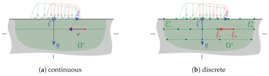
Figure 2. Illustration of the transient step of the residual stress approximation scheme as a continuous process (a) and as a corresponding discrete increment (b). The green dots in (b) represent the spatial discretization ${\Omega }_{\mathrm{d}}^{*}$ of the domain ${\Omega }^{*}$ on which temperature and thermoelastic stresses are assumed to be given as input to the thermoelastoplastic approximation scheme.

To compute the unknown stress components, let us consider a material point moving below the surface loads as shown in Figure 2a and assume an elastoplastic response, i.e., $f=0$ and ${\dot{\sigma }}_{ij}^{\prime }{n}_{ij}^{}-h_{\mathrm{T}}\dot{T}\ge 0$ with f, $n_{ij}$ and $h_{\mathrm{T}}$ defined as in Section 2.1. Then, the total strain rate is given as the sum of elastic, plastic, and thermal strains,

$$\begin{array}{cc}\hfill {\dot{\epsilon }}_{ij}& =\underset{={\dot{\epsilon }}_{ij}^{\mathrm{e}}}{\underbrace{\phantom{\frac{1}{h_{\epsilon }}}\frac{1}{E}({\dot{\sigma }}_{ij}-\nu \left({\dot{\sigma }}_{kk}{\delta }_{ij}-{\dot{\sigma }}_{ij}\right))}}+\underset{={\dot{\epsilon }}_{ij}^{\mathrm{p}}}{\underbrace{\frac{1}{h_{\epsilon }}\left({\dot{\sigma }}_{kl}^{\prime }{n}_{kl}^{}-h_{\mathrm{T}}\dot{T}\right)n_{ij}}}+\underset{={\dot{\epsilon }}_{ij}^{\mathrm{th}}}{\underbrace{\phantom{\frac{1}{h_{\epsilon }}}\alpha \dot{T}{\delta }_{ij}}},\hfill \end{array}$$

(13)

where the isotropic Hooke’s law, the flow rule Equation (8) and linear isotropic thermal expansion have been employed for the elastic, plastic and thermal strain rates, respectively. E, $\nu$, and $\alpha$ denote Young’s modulus, Poisson’s ratio and the coefficient of thermal expansion.

To treat both methods and their respective conditions, Equations (11) and (12), in a unified formalism, we now adopt the notation proposed by McDowell [8], so that the MM and JS schemes may be recovered by setting $\Psi =0$ or $\Psi =1$, respectively, in the derivations to follow. Then, the conditions ${\dot{\epsilon }}_{\xi \xi }=0$ (MM, $\Psi =0$) and ${\dot{\sigma }}_{\xi \xi }={\dot{\sigma }}_{\xi \xi }^{*}$ (JS, $\Psi =1$) can be summarized to the single equation

$$\begin{array}{ccc}\hfill {\dot{\epsilon }}_{\xi \xi }& =\hfill & \frac{1}{E}\left({\dot{\sigma }}_{\xi \xi }-\nu \left({\dot{\sigma }}_{\zeta \zeta }+{\dot{\sigma }}_{\eta \eta }^{*}\right)\right)+\frac{1}{h_{\epsilon }}\left({\dot{\sigma }}_{\xi \xi }{n}_{\xi \xi }+{\dot{\sigma }}_{\zeta \zeta }{n}_{\zeta \zeta }+{\dot{\sigma }}_{\eta \eta }^{*}{n}_{\eta \eta }+{\dot{\sigma }}_{\xi \eta }^{*}{n}_{\xi \eta }-h_{\mathrm{T}}{\dot{T}}^{*}\right)n_{\xi \xi }+\alpha {\dot{T}}^{*}\hfill \\ \hfill & \stackrel{!}{=}\hfill & \Psi (\frac{1}{E}\left({\dot{\sigma }}_{\xi \xi }^{*}-\nu \left({\dot{\sigma }}_{\zeta \zeta }+{\dot{\sigma }}_{\eta \eta }^{*}\right)\right)+\frac{1}{h_{\epsilon }}\left({\dot{\sigma }}_{\xi \xi }^{*}{n}_{\xi \xi }+{\dot{\sigma }}_{\zeta \zeta }{n}_{\zeta \zeta }+{\dot{\sigma }}_{\eta \eta }^{*}{n}_{\eta \eta }+{\dot{\sigma }}_{\xi \eta }^{*}{n}_{\xi \eta }-h_{\mathrm{T}}{\dot{T}}^{*}\right)n_{\xi \xi }+\alpha {\dot{T}}^{*}).\hfill \end{array}$$

(14)

Note that ${\dot{\sigma }}_{\xi \xi }$ is replaced by ${\dot{\sigma }}_{\xi \xi }^{*}$ in the otherwise identical sum in the second line. The plane-strain kinematic constraint yields

$$\begin{array}{c}\hfill 0\stackrel{!}{=}{\dot{\epsilon }}_{\zeta \zeta }=\frac{1}{E}\left({\dot{\sigma }}_{\zeta \zeta }-\nu \left({\dot{\sigma }}_{\xi \xi }+{\dot{\sigma }}_{\eta \eta }^{*}\right)\right)+\frac{1}{h_{\epsilon }}\left({\dot{\sigma }}_{\xi \xi }{n}_{\xi \xi }+{\dot{\sigma }}_{\zeta \zeta }{n}_{\zeta \zeta }+{\dot{\sigma }}_{\eta \eta }^{*}{n}_{\eta \eta }+{\dot{\sigma }}_{\xi \eta }^{*}{n}_{\xi \eta }-h_{\mathrm{T}}{\dot{T}}^{*}\right)n_{\zeta \zeta }+\alpha {\dot{T}}^{*}.\end{array}$$

(15)

For an elastic response, i.e., if either $f<0$ or $f=0$ and ${\dot{\sigma }}_{ij}^{\prime }{n}_{ij}^{}-h_{\mathrm{T}}\dot{T}<0$, we can obtain the corresponding equations by simply dropping all terms related to the plastic strain rate ${\dot{\epsilon }}_{ij}^{\mathrm{p}}$ from Equations (13)–(15).

Ideally, the differential equation system (14) and (15)—or its particularization for elastic behavior—should at each arbitrary but fixed depth $\eta$ be integrated w.r.t. $\xi$ from a stress-free initial state to a stress free stationary state of the elastic solution, i.e., within bounds $\xi ={\xi }_{+\infty }^{*}$ and $\xi ={\xi }_{-\infty }^{*}\le {\xi }_{+\infty }^{*}$ sufficiently far away from the surface loads so that the stress ${\sigma }_{ij}^{*}$ of the elastic solution has decayed to zero. Thus, the residual stress approximation ${\sigma }_{ij}^{\mathrm{r}}$ obtained by such an integration will by virtue of Equations (11) and (12) satisfy the conditions on the stresses that are required for homogeneity in the $\xi$-direction in a plane strain half-space problem [5],

$$\begin{array}{c}\hfill {\sigma }_{\eta \eta }^{\mathrm{r}}\stackrel{!}{=}0\mathrm{and}{\sigma }_{\xi \eta }^{\mathrm{r}}\stackrel{!}{=}0.\end{array}$$

(16)

Additionally, as noted by Merwin and Johnson [5], the residual strains have to satisfy the conditions

$$\begin{array}{c}\hfill {\epsilon }_{\xi \xi }^{\mathrm{r}}\stackrel{!}{=}0\mathrm{and}{\epsilon }_{\zeta \zeta }^{\mathrm{r}}\stackrel{!}{=}0.\end{array}$$

(17)

The condition on the residual strain ${\epsilon }_{\xi \xi }^{\mathrm{r}}$ will only be guaranteed for the MM approach but not for the method of JS; compare Equations (11) and (12). Furthermore, since the JS approach enforces ${\sigma }_{\xi \xi }={\sigma }_{\xi \xi }^{*}$, the corresponding residual stress component will generally not be approximated well but vanish after a complete pass below the loaded region. Finally, if we chose to integrate only to ${\xi }_{-}^{*}>{\xi }_{-\infty }^{*}$ where the stress ${\sigma }_{ij}^{*}$ is not yet fully decayed to zero, but already sufficiently so as to not sustain any further plastic response, there will in any case be some violation of Equation (16). For these reasons, the following additional “relaxation” procedure has been proposed (in similar form) as a subsequent step to the integration of above differential equations [7,9]:

With ${\overline{\sigma }}_{ij}$, ${\overline{\epsilon }}_{ij}$, $\overline{T}$, and ${\overline{\epsilon }}^{\mathrm{eq}}$ denoting the state after the above integration for each depth $\eta$ considered, the in-plane stresses and strains required to vanish by the conditions (16) and (17) are assumed to be relaxed to zero at constant rates

$$\begin{array}{c}\hfill {\dot{\sigma }}_{\eta \eta }\stackrel{!}{=}{\dot{\sigma }}_{\eta \eta }^{\mathrm{R}}:=-\frac{{\overline{\sigma }}_{\eta \eta }}{{\tau }^{\mathrm{R}}},{\dot{\sigma }}_{\xi \eta }\stackrel{!}{=}{\dot{\sigma }}_{\xi \eta }^{\mathrm{R}}:=-\frac{{\overline{\sigma }}_{\xi \eta }}{{\tau }^{\mathrm{R}}},{\dot{\epsilon }}_{\xi \xi }\stackrel{!}{=}{\dot{\epsilon }}_{\xi \xi }^{\mathrm{R}}:=-\frac{{\overline{\epsilon }}_{\xi \xi }}{{\tau }^{\mathrm{R}}}\mathrm{and}\dot{T}\stackrel{!}{=}{\dot{T}}^{\mathrm{R}}:=-\frac{\overline{T}}{{\tau }^{\mathrm{R}}},\end{array}$$

(18)

over an interval $[0,{\tau }^{\mathrm{R}}]$ of pseudo-time ${\tau }^{\mathrm{R}}>0$ while the stresses ${\sigma }_{\xi \xi }$ and ${\sigma }_{\zeta \zeta }$ are obtained by integration of the differential equation system

$$\begin{array}{cc}\hfill {\dot{\epsilon }}_{\xi \xi }^{\mathrm{R}}\stackrel{!}{=}& {\dot{\epsilon }}_{\xi \xi }=\frac{1}{E}\left({\dot{\sigma }}_{\xi \xi }-\nu \left({\dot{\sigma }}_{\zeta \zeta }+{\dot{\sigma }}_{\eta \eta }^{\mathrm{R}}\right)\right)+\frac{1}{h_{\epsilon }}\left({\dot{\sigma }}_{\xi \xi }{n}_{\xi \xi }+{\dot{\sigma }}_{\zeta \zeta }{n}_{\zeta \zeta }+{\dot{\sigma }}_{\eta \eta }^{\mathrm{R}}{n}_{\eta \eta }+{\dot{\sigma }}_{\xi \eta }^{\mathrm{R}}{n}_{\xi \eta }-h_{\mathrm{T}}{\dot{T}}^{\mathrm{R}}\right)n_{\xi \xi }+\alpha {\dot{T}}^{\mathrm{R}}\hfill \end{array}$$

(19)

$$\begin{array}{cc}\hfill 0\stackrel{!}{=}& {\dot{\epsilon }}_{\zeta \zeta }=\frac{1}{E}\left({\dot{\sigma }}_{\zeta \zeta }-\nu \left({\dot{\sigma }}_{\xi \xi }+{\dot{\sigma }}_{\eta \eta }^{\mathrm{R}}\right)\right)+\frac{1}{h_{\epsilon }}\left({\dot{\sigma }}_{\xi \xi }{n}_{\xi \xi }+{\dot{\sigma }}_{\zeta \zeta }{n}_{\zeta \zeta }+{\dot{\sigma }}_{\eta \eta }^{\mathrm{R}}{n}_{\eta \eta }+{\dot{\sigma }}_{\xi \eta }^{\mathrm{R}}{n}_{\xi \eta }-h_{\mathrm{T}}{\dot{T}}^{\mathrm{R}}\right)n_{\zeta \zeta }+\alpha {\dot{T}}^{\mathrm{R}}\hfill \end{array}$$

(20)

in the elastoplastic case, i.e., if $f=0$ and ${\dot{\sigma }}_{ij}^{\prime }{n}_{ij}^{}-h_{\mathrm{T}}\dot{T}\ge 0$. Again, the differential equations for the elastic case are obtained by dropping the summands originating from the plastic strain rate in Equations (19) and (20). We will discuss the integration of the differential equation systems given above in the following section.

2.3. Numerical Integration Scheme

Consider a material point moving at a fixed depth $\eta$ from a grid point ${\xi }_{+}$ of the discretization ${\Omega }_{\mathrm{d}}^{*}$ of ${\Omega }^{*}$, where the thermoelastic solution is given, to the neighboring point ${\xi }_{-}$; see Figure 2b. For this point, the material derivative defined by Equation (1) may be approximated by first order finite differences as

$$\begin{array}{c}\hfill \dot{F}=\frac{\mathrm{D}F}{\mathrm{D}t}=-v\frac{\partial F}{\partial \xi }\approx -v\frac{F^{-}-F^{+}}{{\xi }^{-}-{\xi }^{+}}=-\frac{v}{\Delta \xi }\Delta F\end{array}$$

(21)

for any tensor field F, where we introduced the shorthands ${(•)}^{-}$ and ${(•)}^{+}$ to denote evaluation at ${\xi }^{-}$ and ${\xi }^{+}$, respectively, i.e., $F^{-}=F\left({\xi }^{-}\right)$ and $F^{+}=F\left({\xi }^{+}\right)$. Note that each summand in Equations (14) and (15) contains one rate as a linear factor, so that $-v\Delta {\xi }^{-1}$ may be canceled out after discretizing each rate according to Equation (21). Therefore, the rate operators in Equations (14) and (15) reduce to difference operators $\Delta (•)={(•)}^{-}-{(•)}^{+}$ in the discretized counterparts. The same reasoning applies for the relaxation step, where we approximate all rates as

$$\begin{array}{c}\hfill \dot{F}\approx \frac{\Delta F}{\Delta \tau },\end{array}$$

(22)

assuming that the relaxation happens in M pseudo-timesteps of size $\Delta \tau ={\tau }^{\mathrm{R}}{M}^{-1}$ and denoting the increment of F during $\Delta \tau$ as $\Delta F$. Again, the simple structure of Equations (19) and (20) as well as the rate-independency of our constitutive assumptions allow to cancel the increment size, i.e., $\Delta \tau$.

This discretization amounts to applying either explicit or implicit Euler integration if the remaining quantities are all evaluated at the increment’s start or at its end, respectively. For both cases, the solution of an elastoplastic increment is summarized in Algorithms 1 and 2, respectively. We shall discuss them in the context of the complete residual stress approximation scheme, but first, an elastic predictor is required in each increment to determine if the material response actually is elastoplastic or not: Setting $\Delta {\epsilon }_{ij}^{\mathrm{p}}=0$ in the discretized counterparts of Equations (14) and (15), we obtain

$$\begin{array}{cc}\Delta {\epsilon }_{\xi \xi }\hfill & =\frac{1}{E}\left(\Delta {\sigma }_{\xi \xi }-\nu \left(\Delta {\sigma }_{\zeta \zeta }+\Delta {\sigma }_{\eta \eta }^{*}\right)\right)+\alpha \Delta T^{*}\stackrel{!}{=}\Psi \left(\frac{1}{E}\left(\Delta {\sigma }_{\xi \xi }^{*}-\nu \left(\Delta {\sigma }_{\zeta \zeta }+\Delta {\sigma }_{\eta \eta }^{*}\right)\right)+\alpha \Delta T^{*}\right)\hfill \end{array}$$

(23)

$$\begin{array}{cc}\Delta {\epsilon }_{\zeta \zeta }\hfill & =\frac{1}{E}\left(\Delta {\sigma }_{\zeta \zeta }-\nu \left(\Delta {\sigma }_{\xi \xi }+\Delta {\sigma }_{\eta \eta }^{*}\right)\right)+\alpha \Delta T^{*}\stackrel{!}{=}0.\hfill \end{array}$$

(24)

Algorithm 1: Explicit integration of stresses and equivalent plastic strain.

1.     Determine $\Delta {\sigma }_{\xi \xi }$ and $\Delta {\sigma }_{\zeta \zeta }$ by solving the linear equation system: $$\begin{array}{}\begin{array}{ccc}\left(1+\frac{E}{h_{\epsilon }^{+}}{n}_{\xi \xi }^{+}{n}_{\xi \xi }^{+}\right)\Delta {\sigma }_{\xi \xi }\hfill & \hfill +(1-\Psi )\left(-\nu +\frac{E}{h_{\epsilon }^{+}}{n}_{\xi \xi }^{+}{n}_{\zeta \zeta }^{+}\right)\Delta {\sigma }_{\zeta \zeta }=& \hfill \Psi \left(1+\frac{E}{h_{\epsilon }^{+}}{n}_{\xi \xi }^{+}{n}_{\xi \xi }^{+}\right)\Delta {\sigma }_{\xi \xi }^{*}\end{array}\\ \hfill +(\Psi -1)\left(\left(-\nu +\frac{E}{h_{\epsilon }^{+}}{n}_{\xi \xi }^{+}{n}_{\eta \eta }^{+}\right)\Delta {\sigma }_{\eta \eta }^{*}+\frac{2E}{h_{\epsilon }^{+}}{n}_{\xi \xi }^{+}{n}_{\xi \eta }^{+}\Delta {\sigma }_{\xi \eta }^{*}-\left(\frac{E{h}_{\mathrm{T}}^{+}}{h_{\epsilon }^{+}}{n}_{\xi \xi }^{+}-\alpha E\right)\Delta T^{*}\right)\end{array}$$ (25) $$\begin{array}{cc}\left(-\nu +\frac{E}{h_{\epsilon }^{+}}{n}_{\xi \xi }^{+}{n}_{\zeta \zeta }^{+}\right)\Delta {\sigma }_{\xi \xi }\hfill & \hfill +\left(1+\frac{E}{h_{\epsilon }^{+}}{n}_{\zeta \zeta }^{+}{n}_{\zeta \zeta }^{+}\right)\Delta {\sigma }_{\zeta \zeta }=\left(\nu -\frac{E}{h_{\epsilon }^{+}}{n}_{\eta \eta }^{+}{n}_{\zeta \zeta }^{+}\right)\Delta {\sigma }_{\eta \eta }^{*}\\ & -\frac{2E}{h_{\epsilon }^{+}}{n}_{\zeta \zeta }^{+}{n}_{\xi \eta }^{+}\Delta {\sigma }_{\xi \eta }^{*}+\left(\frac{E{h}_{\mathrm{T}}^{+}}{h_{\epsilon }^{+}}{n}_{\zeta \zeta }^{+}-\alpha E\right)\Delta T^{*}\hfill \end{array}$$ (26) 2.     Update the stresses ${\sigma }_{ij}^{-}={\sigma }_{ij}^{+}+\Delta {\sigma }_{ij}$ using the solution from the previous step and $\Delta {\sigma }_{\eta \eta }=\Delta {\sigma }_{\eta \eta }^{*}$ as well as $\Delta {\sigma }_{\xi \eta }=\Delta {\sigma }_{\xi \eta }^{*}$. 3.      Compute approximations of $n_{ij}^{-}$, $h_{\epsilon }^{-}$, and $h_{\mathrm{T}}^{-}$ by Equation (9) with ${\epsilon }^{\mathrm{eq}}={\epsilon }^{\mathrm{eq}+}$, $T=T^{*-}$. 4.      Update the equivalent plastic strain, using $n_{ij}^{-}$, $h_{\epsilon }^{-}$ and $h_{\mathrm{T}}^{-}$ from the previous step: $$\begin{array}{c}\hfill {\epsilon }^{\mathrm{eq}-}\stackrel{\left(10\right)}{=}{\epsilon }^{\mathrm{eq}+}+\sqrt{\frac{2}{3}}\frac{1}{|h_{\epsilon }^{-}|}\left(\Delta {\sigma }_{ij}^{\prime }{n}_{ij}^{-}-h_{\mathrm{T}}^{-}\Delta T^{*}\right)\end{array}$$ (27)

Algorithm 2: Implicit integration of stresses and equivalent plastic strain.

Compute the root $({\sigma }_{\xi \xi }^{-},{\sigma }_{\zeta \zeta }^{-},{\epsilon }^{\mathrm{eq}-})$ of the following nonlinear equation system via Newton–Raphson iteration: $$\begin{array}{cc}\hfill r_{\xi \xi :=}& \left(1+\frac{E}{h_{\epsilon }^{-}}{n}_{\xi \xi }^{-}{n}_{\xi \xi }^{-}\right)\Delta {\sigma }_{\xi \xi }+(1-\Psi )\left(-\nu +\frac{E}{h_{\epsilon }^{-}}{n}_{\xi \xi }^{-}{n}_{\zeta \zeta }^{-}\right)\Delta {\sigma }_{\zeta \zeta }-\Psi \left(1+\frac{E}{h_{\epsilon }^{-}}{n}_{\xi \xi }^{-}{n}_{\xi \xi }^{-}\right)\Delta {\sigma }_{\xi \xi }^{*}\hfill \\ & -(\Psi -1)\left(\left(-\nu +\frac{E}{h_{\epsilon }^{-}}{n}_{\xi \xi }^{-}{n}_{\eta \eta }^{-}\right)\Delta {\sigma }_{\eta \eta }^{*}+\frac{2E}{h_{\epsilon }^{-}}{n}_{\xi \xi }^{-}{n}_{\xi \eta }^{-}\Delta {\sigma }_{\xi \eta }^{*}-\left(\frac{E{h}_{\mathrm{T}}^{-}}{h_{\epsilon }^{-}}{n}_{\xi \xi }^{-}-\alpha E\right)\Delta T^{*}\right),\hfill \end{array}$$ (28) $$\begin{array}{cc}\hfill r_{\zeta \zeta :=}& \left(-\nu +\frac{E}{h_{\epsilon }^{-}}{n}_{\xi \xi }^{-}{n}_{\zeta \zeta }^{-}\right)\Delta {\sigma }_{\xi \xi }+\left(1+\frac{E}{h_{\epsilon }^{-}}{n}_{\zeta \zeta }^{-}{n}_{\zeta \zeta }^{-}\right)\Delta {\sigma }_{\zeta \zeta }-\left(\nu -\frac{E}{h_{\epsilon }^{-}}{n}_{\eta \eta }^{-}{n}_{\zeta \zeta }^{-}\right)\Delta {\sigma }_{\eta \eta }^{*}\hfill \\ & +\frac{2E}{h_{\epsilon }^{-}}{n}_{\zeta \zeta }^{-}{n}_{\xi \eta }^{-}\Delta {\sigma }_{\xi \eta }^{*}-\left(\frac{E{h}_{\mathrm{T}}^{-}}{h_{\epsilon }^{-}}{n}_{\zeta \zeta }^{-}-\alpha E\right)\Delta T^{*},\hfill \end{array}$$ (29) $$\begin{array}{cc}\hfill r_f& :=n_{ij}^{-}{n}_{ij}^{-}-1,\hfill \end{array}$$ (30) where $\Delta {\sigma }_{\xi \xi }={\sigma }_{\xi \xi }^{-}-{\sigma }_{\xi \xi }^{+}$, $\Delta {\sigma }_{\zeta \zeta }={\sigma }_{\zeta \zeta }^{-}-{\sigma }_{\zeta \zeta }^{+}$ and $n_{ij}^{-}$, $h_{\epsilon }^{-}$ and $h_{\mathrm{T}}^{-}$ are evaluated using the current Newton iteration’s approximation of the root.

Then, the predictor stress increment $\Delta {\sigma }_{ij}^{\mathrm{pr}}$ is obtained by solving this linear equation system, which we will more generically denote by using the operator P defined as

$$\begin{array}{c}\hfill P(\Delta {\sigma }_{ij}^{*},\Delta T,\Psi )=\Delta {\sigma }_{ij}^{\mathrm{pr}}\end{array}$$

(31)

wherein the stress components are related by

$$\begin{array}{cccc}\hfill \Delta {\sigma }_{\xi \xi }^{\mathrm{pr}}& =-\frac{(\Psi -1)\nu (\nu +1)\Delta {\sigma }_{\eta \eta }^{*}-\Psi \Delta {\sigma }_{\xi \xi }^{*}-(\Psi -1)(1+\nu )\alpha E\Delta T^{*}}{(\Psi -1){\nu }^2+1},\hfill & \hfill \Delta {\sigma }_{\eta \eta }^{\mathrm{pr}}& =\Delta {\sigma }_{\eta \eta }^{*},\hfill \end{array}$$

(32)

$$\begin{array}{cccc}\hfill \Delta {\sigma }_{\zeta \zeta }^{\mathrm{pr}}& =-\frac{\nu \left((\Psi -1)\nu -1\right)\Delta {\sigma }_{\eta \eta }^{*}-\Psi \nu \Delta {\sigma }_{\xi \xi }^{*}+\left(1-\nu (\Psi -1)\right)\alpha E\Delta T^{*}}{(\Psi -1){\nu }^2+1},\hfill & \hfill \Delta {\sigma }_{\xi \eta }^{\mathrm{pr}}& =\Delta {\sigma }_{\xi \eta }^{*}.\hfill \end{array}$$

(33)

Note that we may reuse this operator P to generically denote the solution of Equations (23) and (24) for arbitrary given increments—or even absolute values—of the stress and the temperature.

For the relaxation step, a predictor may analogously be derived by setting $\Delta {\epsilon }_{ij}^{\mathrm{p}}=0$ in the discretized versions of Equations (19) and (20), in which the rates prescribed by Equation (18) reduce to the increments

$$\begin{array}{c}\hfill \Delta {\sigma }_{\eta \eta }^{\mathrm{R}}=-{\overline{\sigma }}_{\eta \eta }{M}^{-1},\Delta {\sigma }_{\xi \eta }^{\mathrm{R}}=-{\overline{\sigma }}_{\xi \eta }{M}^{-1},\Delta {\epsilon }_{\xi \xi }^{\mathrm{R}}=-{\overline{\epsilon }}_{\xi \xi }{M}^{-1}\mathrm{and}\Delta T^{\mathrm{R}}=-\overline{T}{M}^{-1}.\end{array}$$

(34)

Again, the predictor stress increment $\Delta {\sigma }_{ij}^{\mathrm{pr}\mathrm{R}}$ is obtained by solving the resulting linear equation system,

$$\begin{array}{cc}\Delta {\sigma }_{\xi \xi }^{\mathrm{pr}\mathrm{R}}=\frac{1}{1-\nu }\left(\nu \Delta {\sigma }_{\eta \eta }^{\mathrm{R}}+\frac{E\Delta {\epsilon }_{\xi \xi }^{\mathrm{R}}}{\nu +1}-\alpha E\Delta T^{\mathrm{R}}\right),\hfill & \Delta {\sigma }_{\eta \eta }^{\mathrm{pr}\mathrm{R}}=\Delta {\sigma }_{\eta \eta }^{\mathrm{R}},\hfill \end{array}$$

(35)

$$\begin{array}{cc}\Delta {\sigma }_{\zeta \zeta }^{\mathrm{pr}\mathrm{R}}=\Delta {\sigma }_{\xi \xi }^{\mathrm{pr}\mathrm{R}}-\frac{E}{1+\nu }\Delta {\epsilon }_{\xi \xi }^{\mathrm{R}},\hfill & \Delta {\sigma }_{\xi \eta }^{\mathrm{pr}\mathrm{R}}=\Delta {\sigma }_{\xi \eta }^{\mathrm{R}}.\hfill \end{array}$$

(36)

Note that this predictor is constant throughout the relaxation.

The complete residual stress approximation scheme can now be assembled based on the previous definitions and derivations of this chapter; see Figure 3 for the corresponding flow chart, which shall be discussed in the following:

• First, we note that this computational routine needs to be repeated for each individual depth $\eta$ under consideration. However, since there is no direct coupling between the depths, but only indirect coupling through the elastic solution, this may be done in parallel. Generally, since stress and temperature in the elastic solution decay with distance from the loaded strip, a load imbalance should be expected when parallelizing the evaluation of different depths.
• Initial conditions for the stress and equivalent plastic strain are set at the upmost ${\xi }_{+}^{*}$ seen in Figure 2b. For efficiency, ${\xi }_{+}^{*}$ shall be set as close as possible to the surface loads while asserting that no plasticity occurs for $\xi >{\xi }_{+}^{*}$. Thus, ${\epsilon }^{\mathrm{eq}+}=0$ and given that there is no path dependency in the elastic regime, the stress can be initialized by applying the P operator Equation (31), as seen in Figure 3, which effectively yields an equivalent initial state as we would eventually obtain when starting the integration much further away just to ensure ${\sigma }_{ij}^{+}\approx 0$ initially.
• With the loop construct in the left of Figure 3, we then proceed through the loaded region in (not necessarily constant) increments of $\Delta \xi$, see Figure 2b, thus reconstructing the transient loading history a material point would be subjected to in the elastic moving surface load problem. In doing so, the elastoplastic material response is approximated within the assumptions Equations (11) or (12) by a predictor–corrector approach. Elastoplastic increments are solved using either explicit or implicit integration, as detailed in Algorithms 1 and 2, respectively.
• While the strains generally do not have to be computed explicitly during this first part of the scheme, which is entirely formulated in terms of stresses, all strain components can easily be updated at the end of each increment based on the discretized version of Equation (13). However, doing so is only strictly necessary for ${\epsilon }_{\xi \xi }$, since the only strain component required in the overall scheme is ${\overline{\epsilon }}_{\xi \xi }$, for which Equation (17) has to be checked prior to potentially invoking the relaxation step.
• Similarly as discussed for the initial condition, it is desirable for efficiency reasons to choose the value of ${\xi }_{-}^{*}$, where the integration is stopped, not too far away from the surface loads. Since the elastic solution does satisfy the Merwin–Johnson conditions Equations (16) and (17) for $\xi \to -\infty$, which the relaxation eventually enforces, path independency in the elastic regime allows not only a coarsening of the integration step length beyond the plastic zone but also using the relaxation procedure earlier, i.e., starting at larger ${\xi }_{-}^{*}$, to attain the conforming steady state instead of continuing integration toward some ${\xi }_{-}^{*}$ excessively far away from the loads. However, this reasoning is only admissible if elastic behavior is guaranteed beyond $\xi <{\xi }_{-}^{*}$ and likewise during relaxation from ${\xi }_{-}^{*}$ onward.
• As indicated above, the Merwin–Johnson conditions are checked for ${\overline{\sigma }}_{\eta \eta }$, ${\overline{\sigma }}_{\xi \eta }$ and ${\overline{\epsilon }}_{\xi \xi }$ that result at ${\xi }_{-}^{*}$ from the first step of the scheme. If the check fails, the conditions are enforced by reducing the involved stress and strain components to zero in M increments. Since plasticity may occur during relaxation, M should be sufficiently large to track the associated loading path dependency.
• A very similar predictor–corrector scheme as before is employed during relaxation. However, due to the different set of prescribed stress and strain components, the equations for an elastoplastic relaxation increment differ slightly from the corresponding equations in the previous step of the scheme. Therefore, we collected them in Algorithm 3. Note that we limit the discussion to the case of explicit integration here, since M may conveniently be increased for accuracy, while decreasing $\Delta \xi$ during the first step would come at the possibly large additional cost of further evaluations of the elastic input solution.

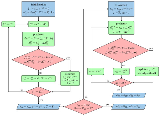
Figure 3. Flow chart for the residual stress approximation.

We conclude the presentation with the remark that the temperature, which is known beforehand, may always be inserted with its value at the increment’s end—even in the explicit integration procedures of Algorithms 1 and 3—which we did in the studies presented in the remainder of the work.

Algorithm 3: Integration of stresses and equivalent plastic strain during relaxation.

1.    Determine $\Delta {\sigma }_{\xi \xi }$ and $\Delta {\sigma }_{\zeta \zeta }$ by solving the linear equation system $$\begin{array}{}\begin{array}{ccc}\left(1+\frac{E}{h_{\epsilon }}{n}_{\xi \xi }{n}_{\xi \xi }\right)\Delta {\sigma }_{\xi \xi }\hfill & \hfill +\left(-\nu +\frac{E}{h_{\epsilon }}{n}_{\xi \xi }{n}_{\zeta \zeta }\right)\Delta {\sigma }_{\zeta \zeta }=& \hfill \left(\nu -\frac{E}{h_{\epsilon }}{n}_{\xi \xi }{n}_{\eta \eta }\right)\Delta {\sigma }_{\eta \eta }^{\mathrm{R}}\end{array}\\ -\frac{2E}{h_{\epsilon }}{n}_{\xi \xi }{n}_{\xi \eta }\Delta {\sigma }_{\xi \eta }^{\mathrm{R}}+\left(\frac{E{h}_{\mathrm{T}}}{h_{\epsilon }}{n}_{\xi \xi }-\alpha E\right)\Delta T^{\mathrm{R}}+E\Delta {\epsilon }_{\xi \xi }^{\mathrm{R}},\end{array}$$ (37) $$\begin{array}{cc}\left(-\nu +\frac{E}{h_{\epsilon }}{n}_{\xi \xi }{n}_{\zeta \zeta }\right)\Delta {\sigma }_{\xi \xi }\hfill & \hfill +\left(1+\frac{E}{h_{\epsilon }}{n}_{\zeta \zeta }{n}_{\zeta \zeta }\right)\Delta {\sigma }_{\zeta \zeta }=\left(\nu -\frac{E}{h_{\epsilon }}{n}_{\eta \eta }{n}_{\zeta \zeta }\right)\Delta {\sigma }_{\eta \eta }^{\mathrm{R}}\\ & \hfill -\frac{2E}{h_{\epsilon }}{n}_{\zeta \zeta }{n}_{\xi \eta }\Delta {\sigma }_{\xi \eta }^{\mathrm{R}}+\left(\frac{E{h}_{\mathrm{T}}}{h_{\epsilon }}{n}_{\zeta \zeta }-\alpha E\right)\Delta T^{\mathrm{R}},\end{array}$$ (38)    where the stress and equivalent plastic strain assume their values at the relaxation increment’s beginning. 2.     Update the stresses ${\sigma }_{ij}={\sigma }_{ij}+\Delta {\sigma }_{ij}$ using the solution from the previous step and $\Delta {\sigma }_{\eta \eta }=\Delta {\sigma }_{\eta \eta }^{\mathrm{R}}$ as well as $\Delta {\sigma }_{\xi \eta }=\Delta {\sigma }_{\xi \eta }^{\mathrm{R}}$. 3.     Update $n_{ij}$, $h_{\epsilon }$ and $h_{\mathrm{T}}$ by Equation (9) using the updated stress. 4.     Update the equivalent plastic strain using $\Delta {\sigma }_{ij}$, $n_{ij}$, $h_{\epsilon }$ and $h_{\mathrm{T}}$ from the previous two steps, $$\begin{array}{c}\hfill {\epsilon }^{\mathrm{eq}}\stackrel{\left(10\right)}{=}{\epsilon }^{\mathrm{eq}}+\sqrt{\frac{2}{3}}\frac{1}{|h_{\epsilon }|}\left(\Delta {\sigma }_{ij}^{\prime }{n}_{ij}-h_{\mathrm{T}}\Delta T^{\mathrm{R}}\right).\end{array}$$ (39)

3. Finite Element Modeling

This section is devoted to the presentation of the FE models that we established in order to assess the correctness of our implementation of the numerical scheme derived in Section 2 as well as the accuracy of the obtained approximations for half-space problems, as shown in Figure 1. The FE analyses were carried out using Abaqus/Standard (v6.20).

Figure 4 shows a sketch of the “global” FE model used both to obtain the elastic input ${\sigma }_{ij}^{*}$ in a thermoelastic analysis as well as to compute reference solutions for transient and residual stresses in a thermoelastoplastic analysis for comparison with the approximations obtained by the MM and JS methods. We enforced homogeneous displacement boundary conditions w.r.t. the normal direction on the left, right and bottom boundaries. In order to attain half-space conditions for our domain of interest despite these boundary conditions, we assured that the boundaries are sufficiently far away to match the results of simulations in which a boundary layer of CINPE4 infinite plane-strain elements was used. This was not done per default, since the use of infinite elements prevents parallel execution in Abaqus/Standard, leading to significantly higher runtimes while providing no additional accuracy once sufficient distance of the boundaries is established. To apply the moving surface loads and heat flux, the given distributions $t_{\eta \eta }^{*}\left(\xi \right)$, $t_{\xi \eta }^{*}\left(\xi \right)$, and $q^{*}\left(\xi \right)$ seen in Figure 1 were related to the material x–y-system by a Galilean transformation to obtain mechanically equivalent (pseudo)-time-dependent nodal forces $F_{\eta \eta }^{*}\left(t\right)$, $F_{\xi \eta }^{*}\left(t\right)$, and a surface heat flux $Q^{*}\left(t\right)$, which are then prescribed onto the surface of the thermoelastoplastic domain in Figure 4. We implemented this using the Abaqus/Standard user subroutines UTRACLOAD and DFLUX. As indicated, we used this FE model for the following three purposes, adapting the particular dimensions and mesh refinement controls to the requirements of each analysis:

• The elastic solution ${\sigma }_{ij}^{*}$, $T^{*}$, is computed using a transient thermomechanical analysis where thermoelastic material behavior is assumed throughout. The loads are moved over a sufficiently large distance of the model’s surface so that we approximately obtain quasi-stationary fields around the loaded region in a co-moving coordinate system. Then, the analysis is stopped without relieving the mechanical loads or allowing temperature equalization such that we can directly extract the transient loading a material point would be subjected to when passing the loaded region under the preclusion of plasticity.
• To obtain the transient elastoplastic reference solution for material points passing under the surface loads, the above analysis is repeated with thermoelastoplastic material behavior.
• To compute the residual stresses, another thermoelastoplastic analysis is conducted, where the loads are relieved and the temperature is equalized in an additional transient simulation step.

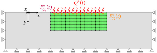
Figure 4. Sketch of the FE model for the half-space problem of Figure 1. The domain of interest, where thermoelastoplastic material behavior is applied, is shown in green and is discretized with a structured mesh of plane-strain elements. The surrounding gray area serves as thermoelastic embedding and is discretized by an unstructured mesh of plane-strain elements (omitted in the sketch) that progressively coarsens toward the outer boundaries that confine the half-space.

These FE simulations provide us with reference solutions to assess the quality of results obtained by the methods of Section 2. However, they are not suitable to validate our implementation of the approximate algorithms, since deviations arising from the “depth-uncoupled” nature of the MM and JS methods as well as from the assumptions Equations (11) and (12) cannot be distinguished from other potential discrepancies.

For this purpose, the two simple FE models shown in Figure 5 were established. They each consist of a single plane-strain finite element with boundary conditions, nodal forces, surface tractions and temperature prescribed specifically so as to impose the kinematic constraints and the elastic stress components defined by Equations (11) and (12). By appropriate definition of the temporal evolution of these loads, we can simulate the thermoelastoplastic behavior of a single material point for arbitrary loading histories under the exact mechanical assumptions of MM and JS using the constitutive models included in Abaqus. This is easily implemented using the UEXTERNALDB and UAMP subroutines to load and apply the desired time series. In particular, by prescribing the solution from the elastic analysis of the “global” model seen in Figure 4, validation data for the MM and JS methods can be computed for general half-space problems, as sketched in Figure 1. An analogous model can be build for the relaxation step of the approximate algorithms, where the strain in the $\xi$-direction is enforced by an appropriate displacement boundary condition.

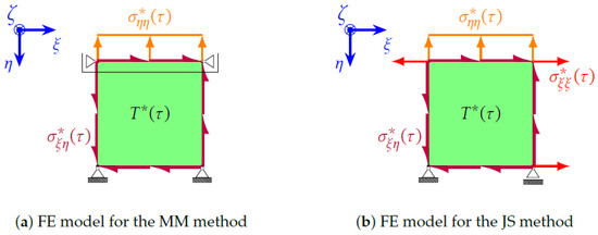
Figure 5. FE models used to validate our implementation of the approximation schemes’ transient step. $\tau$ denotes the (pseudo-)time during the transient analysis. The bar connecting the bearings at the top two nodes in subfigure (a) represents a multi-point constraint that enforces equal displacement in the $\xi$-direction. ${\sigma }_{\eta \eta }^{*}\left(\tau \right)$ and ${\sigma }_{\xi \eta }^{*}\left(\tau \right)$ are prescribed by surface traction definitions in Abaqus while three nodal forces are defined to enforce ${\sigma }_{\xi \xi }^{*}\left(\tau \right)$ for the JS case.

4. Numerical Study and Validation of the Algorithms’ Implementations

This section covers our numerical studies using the approximate algorithms and discusses them in comparison to reference results computed by the FEM. Specifically, we start by validating the implementations using the models shown in Figure 5 and then move on to elaborate on the accuracy of the approximate methods based on the reference solutions from the FE model seen in Figure 4.

To specify the strain-hardening and thermal-softening behavior for our investigations, we assume the following rate-independent Johnson–Cook type law for the yield strength ${\sigma }_{\mathrm{Y}}$:

$$\begin{array}{c}\hfill {\sigma }_{\mathrm{Y}}({\epsilon }^{\mathrm{eq}},T)=\left({\sigma }_{\mathrm{Y}}^0+h{\left({\epsilon }^{\mathrm{eq}}\right)}^n\right)\left(1-{\left(\Theta \left(T\right)\right)}^m\right).\end{array}$$

(40)

Herein, ${\sigma }_{\mathrm{Y}}^0$ is the initial yield strength below or at the transition temperature $T_{\mathrm{t}}$, at which thermal softening is assumed to begin, and prior to strain hardening. The constants h and n determine the slope and nonlinearity of the strain-hardening curve for a given temperature. Thermal softening is accounted for by the second factor in Equation (40) and parameterized by the constant exponent m as well as a function $\Theta \left(T\right)$ defined by

$$\begin{array}{c}\hfill \Theta \left(T\right)=\left\{\begin{array}{cc}0\hfill & \mathrm{for}T<T_{\mathrm{t}}\hfill \\ \frac{T-T_{\mathrm{t}}}{T_{\mathrm{m}}-T_{\mathrm{t}}}\hfill & \mathrm{for}{T}_{\mathrm{t}}\le T\le T_{\mathrm{m}}\hfill \\ 1\hfill & \mathrm{else},\hfill \end{array}\right.\end{array}$$

(41)

where $T_{\mathrm{m}}$ denotes the melting temperature at which the yield strength vanishes. The complete set of constitutive parameters is collected in Table 1. Note that in addition to the parameters introduced before, we included the parameters needed to solve the linear heat conduction problem during the thermoelastic analysis for the input solution ${\sigma }_{ij}^{*}$, $T^{*}$, at the bottom of the table.

Table 1. Baseline constitutive parameters for our numerical investigations if not specified otherwise.

Symbol	Value	Unit	Description
E	113.8	$\mathrm{G}\mathrm{Pa}$	Young’s modulus
$\nu$	0.342		Poisson’s ratio
$\alpha$	9.0 × 10−6	K−1	coefficient of thermal expansion
${\sigma }_{\mathrm{Y}}^0$	920	$\mathrm{M}\mathrm{Pa}$	initial yield stress
h	185	$\mathrm{M}\mathrm{Pa}$	hardening slope
n	0.3		strain-hardening exponent
$T_{\mathrm{t}}$	20	${}^{\circ }\mathrm{C}$	transition temperature
$T_{\mathrm{m}}$	1650	${}^{\circ }\mathrm{C}$	melting temperature
m	1		thermal-softening exponent
$\rho$	4420	kg m−3	density
$\lambda$	6.7	W m−1 K−1	thermal conductivity
$c_{\mathrm{p}}$	526.3	J kg−1 K−1	specific heat capacity
$T_{\infty }$	20	${}^{\circ }\mathrm{C}$	ambient temperature

4.1. Validation of the Approximate Algorithms’ Implementation

For the scope of this section, we consider synthetically defined time evolutions for the prescribed loads on the FE models seen in Figure 5. This simplifies the discussion and the increment size selection for the integration in the approximate algorithms, but more importantly, it allows us to easily assert that the thermoelastic input solution indeed complies with the additional kinematic constraint ${\epsilon }_{\xi \xi }=0$ underlying the MM method. Therefore, it is guaranteed that the validation is done under circumstances where the MM and JS approaches constitute no approximation but exact methods from a mechanical viewpoint; i.e., any deviations from the FE results must be of numerical or implementational origin.

To expand on this point, note that the plane-strain constraint ${\epsilon }_{\zeta \zeta }=0$ by virtue of the thermoelastic extension of Hooke’s law dictates

$$\begin{array}{c}\hfill {\sigma }_{\zeta \zeta }^{*}=\nu \left({\sigma }_{\xi \xi }^{*}+{\sigma }_{\eta \eta }^{*}\right)-\alpha E{T}^{*}\end{array}$$

(42)

and additionally enforcing ${\epsilon }_{\xi \xi }=0$ then leaves us with only one of the two in-plane normal stresses as independent component, i.e., the relation

$$\begin{array}{c}\hfill {\sigma }_{\xi \xi }^{*}=\frac{\nu (1-\nu ){\sigma }_{\eta \eta }^{*}-\alpha E(\nu +1)T^{*}}{1-{\nu }^2}\end{array}$$

(43)

must be taken into account when defining an elastic input solution for the MM algorithm. The FE analysis of the model in Figure 5a will of course result in a compliant $\xi \xi$-component of the stress tensor by itself, but for the approximate algorithm, we must completely define ${\sigma }_{ij}^{*}\left(\tau \right)$ ourselves beforehand.

Since the constitutive behavior is rate-independent, we consider a step of unit pseudo-time $\tau \in [0,1]$ over which we ramp up the temperature $T^{*}\left(\tau \right)$ linearly from 0 to 700 °C. This leads to a maximum reduction of the yield stress of around 40% due to thermal softening as per the second factor in Equation (40). Then, we consider a complete loading–unloading cycle for each individual load sketched in Figure 5 in a separate analysis by prescribing a hat function for the load’s temporal evolution: For both the JS and the MM algorithm, this comprises two analyses in each of which either ${\sigma }_{\eta \eta }^{*}\left(\tau \right)$ or ${\sigma }_{\xi \eta }^{*}\left(\tau \right)$ is prescribed by a hat function. An additional analysis in which ${\sigma }_{\xi \xi }^{*}\left(\tau \right)$ assumes a hat-shaped loading–unloading cycle is carried out for the JS method.

Figure 6 and Figure 7 show the stresses obtained by these analyses, where we used explicit integration (Algorithm 1) with a timestep of $\Delta \tau =$ 1 × 10⁻³. We omit displaying the stresses we correspondingly obtained by implicit integration (Algorithm 2), as they are virtually identical to the results of Algorithm 1 shown here. Note the hat-shaped cycles of the prescribed stress components and that we adjusted the corresponding peak values so that the magnitudes of equivalent plastic strain after the loading cycle were similar. Furthermore, by comparing Figure 6a,b, the expected equal behavior w.r.t. the $\xi$- and $\eta$-directions under the assumptions of JS is confirmed. Finally, by comparing the dashed and dotted lines in Figure 6 and Figure 7, we verify that the stress components computed by the approximate algorithms (i.e., ${\sigma }_{\zeta \zeta }$, and for the MM algorithm additionally ${\sigma }_{\xi \xi }$) agree with the results from the FE calculations throughout.

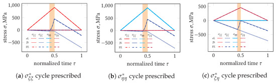
Figure 6. Transient stresses computed by FE analysis vs. the JS method and the prescribed elastic input (labeled “el.” and drawn using dotted lines). The highlighted subinterval of $\tau$ represents the domain where plasticity occurred.

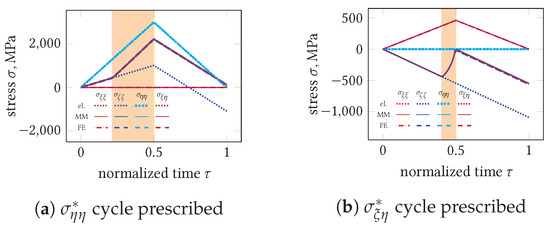
Figure 7. Transient stresses computed by the FE analysis vs. the MM method and the prescribed elastic input (“el.”, dotted lines). Plasticity occurred within the highlighted subinterval of $\tau$.

The total and equivalent plastic strain for the ${\sigma }_{\xi \xi }$ loading cycle of Figure 6a are shown in Figure 8 for the explicit and implicit implementations of the JS algorithm. The observations discussed for this case hold similarly for the other load cycles studied. Comparing to the FE results, it is apparent that a somewhat better agreement in terms of strains is obtained by the implicit integration although it was computed using a four times coarser time discretization $\Delta \tau =$ 4 × 10⁻³. As indicated in Section 2.2, this does not influence the stresses, since the Algorithms 1 and 2 are formulated exclusively in terms of the stresses. The obvious reason for the slightly worse strain approximation of the explicit Algorithm 1 is that the equivalent plastic strain is computed only after the elastoplastic stress correction which involves quantities related to the yield surface at the beginning of the increment. For the same reason, slight violations of the admissibility of the stresses may appear within the explicit scheme. On the other hand, the implicit Algorithm 2 enforces admissibility by updating ${\epsilon }^{\mathrm{eq}}$ during the iteration, resulting in better strain approximations at the general expense of higher computational effort and stronger requirements on the smoothness of the yield surface for convergence.

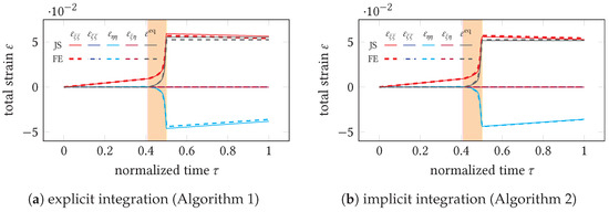
Figure 8. Total and equivalent plastic strain obtained by the FE analysis vs. the results from either the explicit or implicit JS implementation for the loading cycle seen in Figure 6a.

Finally, Figure 9 shows the FE and approximate results for the stresses and strains during the loading-unloading cycle seen in Figure 6a and additionally the subsequent relaxation procedure, in which the Merwin-Johnson conditions and temperature equilibration are enforced incrementally in $M=2500$ steps. The JS case with prescribed ${\sigma }_{\xi \xi }^{*}\left(\tau \right)$ for $\tau \in [0,1]$ was chosen for display here, since it naturally features a large normal strain in $\xi$-direction prior to relaxation and thus constitutes a case where plasticity is predestined to occur in the relaxation step. Indeed, as can be seen from Figure 9, significant plastic flow occurs during relaxation while good agreement of the stresses with the FE results is verified. Since explicit integration is employed for the relaxation (Algorithm 3), the considerations of the previous paragraph on the accuracy of strains apply equally to the moderate deviations observed here.

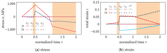
Figure 9. Stress, strain, and equivalent plastic strain evolution according to the FE analysis and the JS algorithm during both the loading cycles seen in Figure 6a and the subsequent relaxation step. Algorithms 2 and 3 were used.

In conclusion, we have provided FE-based validation for each implementational branch of the solution scheme seen in Figure 3 at this point and shall turn our attention to actual half-space problems in the next section.

4.2. Analysis of the Approximation Quality for Half-Space Problems

To study the approximate algorithms in the context of the half-space problem shown in Figure 1, we choose the particular distributions

$$\begin{array}{c}\hfill t_{\eta \eta }^{*}\left(\xi \right)=\left\{\begin{array}{cc}\frac{2p_0^{*}}{\pi b^2}\sqrt{b^2-{\xi }^2}\hfill & \mathrm{for}-b\le \xi \le b\hfill \\ 0\hfill & \mathrm{else}\hfill \end{array}\right.\mathrm{and}{t}_{\xi \eta }^{*}\left(\xi \right)=-\mu t_{\xi \xi }^{*}\left(\xi \right)\end{array}$$

(44)

for the surface loads and for the heat flux distribution, we set

$$\begin{array}{c}\hfill q^{*}\left(\xi \right)=\left\{\begin{array}{cc}{q}_0^{*}\hfill & \mathrm{for}-b\le \xi \le b\hfill \\ 0\hfill & \mathrm{else}.\hfill \end{array}\right.\end{array}$$

(45)

Herein, b denotes the half-width of the loaded area w.r.t. the $\xi$-$\eta$-system and $p_0^{*}$, $q_0^{*}$ and $\mu$ are positive constants. The elliptical pressure distribution in Equation (44) stems from Hertzian contact theory and is very commonly postulated in rolling and sliding contact research. Assuming proportional tangential tractions is known to be somewhat simplistic for sliding contact problems due to the occurrence of both stick and slip regions, but this assumption is widespread nonetheless [7,8]. The authors are aware of existing analytic expressions for the elastic stress solution corresponding to these particular surface tractions [21] as well as the integral given by Carslaw and Jaeger [22] for the temperature field associated with Equation (45). However, it seems that no integral-free, closed-form solution exists for the thermoelastic problem. Therefore, the elastic input solution ${\sigma }_{ij}^{*}$ will be computed by the FEM as described in Section 3, although faster approximate methods [4] or even heuristic approaches [1] are favorable in applications.

The load parameters are chosen as $b=1 \mathrm{m}\mathrm{m}$, $q_0^{*}=1250 \mathrm{k}\mathrm{W}{\mathrm{m}}^{-2}$ and $\mu =0.2$. Furthermore, two levels of intensity are considered for the mechanical loading, $p_0^{*}=1.6 \mathrm{k}\mathrm{N}$ and $p_0^{*}=3.2 \mathrm{k}\mathrm{N}$, so that we may study the algorithms over a wide range of very small to moderately large plastic strains. To extend the range of hardening behavior considered in the investigation, we assume $h\in \left\{2.5,5,10\right\}\mathrm{G}\mathrm{Pa}$ with ${\sigma }_{\mathrm{Y}}^0=920 \mathrm{M}\mathrm{Pa}$ and $n=0.5$. Figure 10 displays the flow curves within the relevant domains of temperature and equivalent plastic strain. Note that the slope of the yield stress w.r.t. the equivalent plastic strain is initially vertical according to Equation (40) if $n<1$ and therefore, $h_{\epsilon }=\infty$ for ${\epsilon }^{\mathrm{eq}}=0$, which is regularized to a large finite value when the explicit Algorithm 1 is employed. Otherwise, $h_{\epsilon }^{+}=\infty$ in the first elastoplastic increment implies $\Delta {\epsilon }_{ij}^{\mathrm{p}}=0$ and ${\epsilon }^{\mathrm{eq}-}={\epsilon }^{\mathrm{eq}+}=0$, so that by induction, it is easily seen that plastic flow would be suppressed within the explicit scheme for this particular choice of hardening behavior. By contrast, the implicit Algorithm 2 requires no special treatment for unbounded $h_{\epsilon }$.

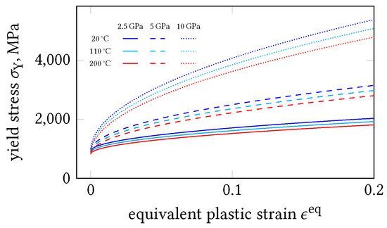
Figure 10. Yield stress as a function of equivalent plastic strain for $h\in \left\{2.5,5,10\right\}\mathrm{G}\mathrm{Pa}$ and three different temperatures.

In the following, a top–down approach will be taken to guide the presentation and discussion of the numerical results, i.e., we consider the residual stresses right away. These are usually the quantities of interest in applications and accordingly the only ones presented in most of the corresponding literature.

4.2.1. MM Method

The residual stresses predicted by the MM method are shown in Figure 11. Comparing the predictions with the corresponding reference solutions computed by the “global” FE model (shown in Figure 4), it is immediately obvious that the approximations are at best of qualitative nature for the cases studied here. In particular, the MM implementation fails to accurately predict the location of the compressive residual stress peak as well as the change to tensile stresses in the immediate subsurface. Looking only at the predicted compressive zone below $\eta =0.1 \mathrm{m}\mathrm{m}$, it is apparent that the compressive peak magnitudes are approximated best in case of $h=10 \mathrm{G}\mathrm{Pa}$ for both studied load amplitudes $p_0^{*}$. Furthermore, with $h=2.5 \mathrm{G}\mathrm{Pa}$, the peak approximation is much worse for the milder loading $p_0^{*}=1.6 \mathrm{k}\mathrm{N}$ than for $p_0^{*}=3.2 \mathrm{k}\mathrm{N}$. This indicates a dependency of the prediction’s accuracy on a combination of loading intensity and hardening behavior. Within the studied parameter space, it seems that larger mechanical loading and strain hardening are advantageous, which—regarding the influence of the loading intensity—agrees with the assessment of McDowell [8] that the MM scheme is unrealistic in case of predominately elastic loading cycles.

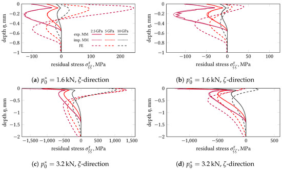
Figure 11. Residual stresses computed by the MM method vs. the results computed by the FEM for various values of the plastic-hardening parameter h and the two considered load levels $p_0^{*}$.

We investigated the sharp reversal of the residual stress approximations near the surface by using once more the “local” FE model of Figure 5a to confirm our implementation’s prediction with a mechanically equivalent FE analysis on a subset of the depths and parameter combinations seen in Figure 11 and found no disagreement. Thus, it seems to us that the poor performance of the MM method in the cases we studied is linked to its inherent mechanical assumptions, as shown in Equation (11). Indeed, enforcing ${\epsilon }_{\xi \xi }={\epsilon }_{\zeta \zeta }=0$ in conjunction with the isotropic constitutive behavior implies equal mechanical response in the $\xi$- and $\zeta$-directions. Accordingly, the predicted residual stress components ${\sigma }_{\xi \xi }^{\mathrm{r}}$ and ${\sigma }_{\zeta \zeta }^{\mathrm{r}}$ are equal, which by itself disagrees in particular in the subsurface tensile region with the FE results; see Figure 11. This deficiency of the MM method was already noted by Jiang and Sehitoglu [7], who study isothermal problems and linear kinematic hardening, and—in accordance with our results—also observed too shallow plastic zones predicted by the MM approach.

A straightforward way to elaborate on the justification of the algorithm’s underlying assumptions is to consider the “true” transient stress and strain components of a material point that passes the loaded region as computed by an elastoplastic FE analysis of the half-space (Figure 4) and to compare them to the respective values prescribed in the models of MM and JS. In particular, we may thus directly examine and compare the validity of the assumptions ${\epsilon }_{\xi \xi }=0$ (MM) and ${\sigma }_{\xi \xi }={\sigma }_{\xi \xi }^{*}$ (JS). Figure 12 displays how the in-plane components of ${\sigma }_{ij}$ obtained by a transient elastoplastic FE analysis deviate from the respective components of the elastic input solution ${\sigma }_{ij}^{*}$ for two of the studied combinations of $p_0^{*}$ and h, which correspond to a “worst-case” scenario (magenta curves in Figure 11a,b, as well as a “best-case” scenario (black curves in Figure 11c,d). Additionally, the elastoplastic FE solution for ${\epsilon }_{\xi \xi }$ is shown. The pseudo-time $\tau$ is used once more to parametrize the temporal course of a point passing the loads. Note that the $\tau$-axis is inverted so that the plotted fields correspond to the problem arrangement defined in Figure 1; i.e., a material point moves from the right to the left in Figure 12. To relate the deviations to the magnitudes of the respective stress components, we normalized them to the peak value of the elastic input solution’s corresponding component that occurs along the considered depth $\eta$; e.g., the absolute difference ${\sigma }_{\xi \eta }^{*}-{\sigma }_{\xi \eta }$ at some fixed point $(\xi ,\eta )\in {\Omega }^{*}$ is normalized by

$$\begin{array}{c}\hfill e_{\eta }({\sigma }_{\xi \eta }^{*},{\sigma }_{\xi \eta }):=\frac{{\sigma }_{\xi \eta }^{*}-{\sigma }_{\xi \eta }}{max\left\{|{\sigma }_{\xi \eta }^{*}(\tilde{\xi },\eta )||\tilde{\xi }\in [{\xi }_{-}^{*},{\xi }_{+}^{*}]\right\}}.\end{array}$$

(46)

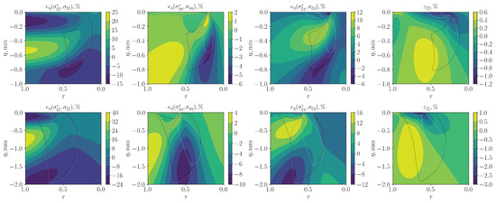
Figure 12. Deviations of the actual stress and strain components involved in the assumptions in Equations (11) and (12) as computed by a transient elastoplastic FE analysis of the half-space model (Figure 4) from their respective target values assumed in the approximate algorithms (top row of plots: $h=2.5 \mathrm{G}\mathrm{Pa}$ and $p_0^{*}=1.6 \mathrm{k}\mathrm{N}$, bottom row: $h=10 \mathrm{G}\mathrm{Pa}$ and $p_0^{*}=3.2 \mathrm{k}\mathrm{N}$). The dashed black and the solid cyan and magenta lines are drawn as rough indicators of the areas where plastic flow occurred as per the FE analysis and the (implicitly integrated) MM and JS algorithms, respectively.

Note that a relative error in the conventional sense cannot be used here, since the stresses may vanish. If the assumptions of MM were to hold rigorously, we should see $e_{\eta }({\sigma }_{\eta \eta }^{*},{\sigma }_{\eta \eta })=e_{\eta }({\sigma }_{\xi \eta }^{*},{\sigma }_{\xi \eta })={\epsilon }_{\xi \xi }\equiv$ 0%. However, the largest violation of the constraint on ${\epsilon }_{\xi \xi }$ is naturally found near the surface where the loads act and the stresses ${\sigma }_{ij}^{*}$ are concentrated. Indeed, we can directly infer from Figure 12 that up to 3% of compressive total strain in the $\xi$-direction are effectively constricted in the near-surface zone by applying the MM scheme, which is accommodated by considerably increased extents of plastic flow compared to the reference FE solution. This coincides with the incorrect prediction of compressive residual stresses building up toward the surface seen in Figure 11. Indeed, we found the severity of the spurious near-surface predictions of the MM method to decrease with smaller violation of the constraint on ${\epsilon }_{\xi \xi }$ throughout all studied cases. Moreover, the depths $\eta$ for which the residual stress predictions are more accurate, i.e., $\eta \approx -0.4 \mathrm{m}\mathrm{m}$ and $\eta \approx -0.5 \mathrm{m}\mathrm{m}$ for the two considered scenarios, respectively, correspond to relatively small violations of this kinematic constraint according to Figure 12.

Obviously, ${\epsilon }_{\xi \xi }=0$ is bound to be a worse assumption for anisothermal problems due to the additional occurrence of hydrostatic thermal strains. Hence, it seems reasonable to expect that their smaller contribution to the overall loading for $p_0^{*}=3.2 \mathrm{k}\mathrm{N}$ promotes the somewhat better predictions in that case, even though it is not trivial to confirm this just by comparing the violation of ${\epsilon }_{\xi \xi }=0$, since increasing the mechanical load simultaneously implies operating with different strain magnitudes and thus, deviations from ${\epsilon }_{\xi \xi }=0$ are harder to interpret when comparing different loading levels.

An important insight provided by Figure 12 is that the deviations from the elastic solution observed for ${\sigma }_{\eta \eta }$ and ${\sigma }_{\xi \eta }$ are substantially smaller than for ${\sigma }_{\xi \xi }$, which corroborates the choice made in both schemes to enforce the elastic solution for the former two stress components. Moreover, the realization that the assumptions on ${\sigma }_{\xi \xi }$ (JS) and ${\epsilon }_{\xi \xi }$ (MM) appear to be considerably more critical as per Figure 12 and the above discussion indicates that both approaches might be justifiable in more specialized loading regimes then the one we study.

Finally, it should be noted that the MM algorithm becomes unstable for weak strain hardening; e.g., for $p_0^{*}=1.6 \mathrm{k}\mathrm{N}$ and $h<2.5 \mathrm{G}\mathrm{Pa}$, we observed increasingly oscillatory distributions of the residual stresses along $\eta$ using explicit integration and accordingly a lack of convergence using implicit integration even though the FE analyses based on the half-space model still yield smooth residual stresses and reasonable maximum equivalent plastic strains. However, since relinquishing kinematic compatibility w.r.t. the $\eta$-direction prevents stress redistribution along the depth, such an unstable plastic response is not entirely unexpected with regard to severe strain localization.

4.2.2. JS Method

The residual stress predictions of the JS method are shown in Figure 13. Much better qualitative agreement with the reference FE solutions is observed compared to the previously discussed MM approach. Both the sign and the peak locations of the residual stress components are mostly well approximated with exception of the lateral component near the surface in Figure 13d for $h<10 \mathrm{G}\mathrm{Pa}$. Moreover, the predicted depth of the zone of non-zero residual stresses agrees reasonably well with the FE results. On the other hand, the peak magnitudes are overestimated in most of the studied cases. As with the MM method, the best agreement is observed for $h=10 \mathrm{G}\mathrm{Pa}$ for both load intensities, which confirms the remark of McDowell [8] that the JS method is expected to perform best for stronger strain hardening, i.e., for larger h. In fact, our results indicate better predictions for larger $h{p_0^{*}}^{-1}$ and demonstrate that excellent residual stress predictions are possible using the JS scheme, as seen for $h=10 \mathrm{G}\mathrm{Pa}$ and $p_0^{*}=1.6 \mathrm{k}\mathrm{N}$ in Figure 13a,b.

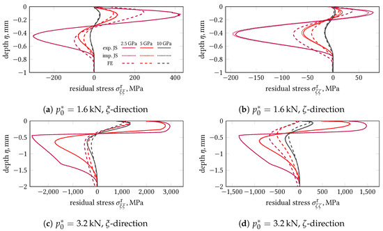
Figure 13. Residual stresses computed by the JS method vs. the results computed by FE analysis for various values of the plastic-hardening parameter h and both considered load levels $p_0^{*}$.

We checked the JS assumption ${\sigma }_{\xi \xi }={\sigma }_{\xi \xi }^{*}$ for all combinations of h and $p_0^{*}$ in the same fashion as we did for the two cases shown in Figure 12, i.e., by comparing the transient stresses occurring during elastoplastic vs. elastic FE analyses of the load passage. The violation of this assumption was found to considerably decrease for fixed $p_0^{*}$ when h is increased, which is unsurprising, since larger h values imply smaller plastic stress relaxation and accordingly stress responses closer to elastic behavior. Furthermore, the quality of the residual stress predictions appears to be linked to the degree of fulfillment of the JS stress constraint, analogously as pointed out above for the MM approach. For example, in case of $p_0^{*}=3.2 \mathrm{k}\mathrm{N}$, deviations $e_{\eta }({\sigma }_{\xi \xi }^{*},{\sigma }_{\xi \xi })$ of more than +75% and +45% were found for $h=2.5 \mathrm{G}\mathrm{Pa}$ and $h=5 \mathrm{G}\mathrm{Pa}$ during plastic flow, respectively, in the depth range where the large overestimation of the compressive residual stresses is seen in Figure 13c,d. At the same time, the constraint violation $e_{\eta }({\sigma }_{\xi \xi }^{*},{\sigma }_{\xi \xi })$ is smaller—and mostly a lot so—than 24% for $h=10 \mathrm{G}\mathrm{Pa}$ within the plastic part of the load passing, as seen in the bottom row of Figure 12. Similarly, the overestimations of the tensile stresses near the surface apparently coincide with significantly larger violations of the shear component assumption ${\sigma }_{\xi \eta }={\sigma }_{\xi \eta }^{*}$ during plastic flow for weaker strain hardening, $h<10 \mathrm{G}\mathrm{Pa}$. Finally, by comparing the diagrams in Figure 12 by row, it is apparent that the assumptions of JS are somewhat better fulfilled for $h=2.5 \mathrm{G}\mathrm{Pa}$ and $p_0^{*}=1.6 \mathrm{k}\mathrm{N}$ than for the other considered parameter set, even though the residual stress approximation is better for the latter. This indicates that higher violations of the JS assumptions may be tolerable with stronger hardening.

To further detail the discussion, we shall examine how the inaccuracies that arise during the load passing step as a consequence of the discussed constraint violations eventually propagate to the residual stress prediction in the course of the relaxation step. To this end, the residual stresses for the cases $h\in \{5,10\}\mathrm{G}\mathrm{Pa}$ and $p_0^{*}=3.2 \mathrm{k}\mathrm{N}$ are once more shown in Figure 14 alongside the corresponding components of the stress ${\overline{\sigma }}_{ij}$ at the end of the loading pass, prior to the relaxation procedure of the JS algorithm. We chose these combinations of h and $p_0^{*}$ since plastic flow during relaxation still occurs for the $h=5 \mathrm{G}\mathrm{Pa}$ case, while the relaxation is entirely elastic for $h=10 \mathrm{G}\mathrm{Pa}$ (which it is also for all the other studied combinations except $p_0^{*}=3.2 \mathrm{k}\mathrm{N}$ with $h=2.5 \mathrm{G}\mathrm{Pa}$). Comparing the dashed lines in Figure 14a,b,d,e, the impact of the JS assumptions’ violations that we pointed out above indeed manifests in the intermediate results ${\overline{\sigma }}_{ij}$, i.e., ${\overline{\sigma }}_{\xi \xi }$ and ${\overline{\sigma }}_{\zeta \zeta }$ deviate from the corresponding FE reference solutions particularly for values of $\eta$ where large violations of the underlying JS assumption on ${\sigma }_{\xi \xi }$ were observed during the loading pass. Furthermore, considering all studied cases, the inaccuracy of ${\overline{\sigma }}_{ij}$ w.r.t. to the FE results was found to become smaller for larger h, as expected according to better fulfillment of Equation (12). However, these inaccuracies seem somewhat less sensitive w.r.t. h as the strong dependency of the residual stress prediction’s accuracy on h suggests for the two parameter combinations considered in Figure 14. On the other hand, looking at Figure 14c,f, the discrepancy of the accuracy of the predicted residual stresses for $h=5 \mathrm{G}\mathrm{Pa}$ and $h=10 \mathrm{G}\mathrm{Pa}$ may be related to the larger straining during relaxation for $h=5 \mathrm{G}\mathrm{Pa}$ due to the much bigger ${\overline{\epsilon }}_{\xi \xi }$ which is forced to zero and correspondingly drives the transient loading during relaxation; see Equations (34) and (37). This assessment seems to be supported by the remark McDowell [8] gave in passing that large magnitudes of relaxation may be the cause of the JS algorithm’s instability for weak hardening. However, since the strains are computed from the stress updates in Algorithms 1 and 2, deviations of ${\overline{\epsilon }}_{\xi \xi }$ from the FE reference strain ultimately relate back to inaccurate stresses obtained during the loading pass and thus to the appropriateness of the assumptions Equation (12).

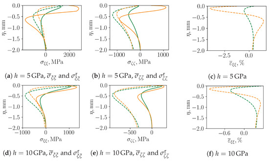
Figure 14. Left and middle column: Depth profiles of the residual stresses ${\sigma }_{\xi \xi }^{\mathrm{r}}$, ${\sigma }_{\zeta \zeta }^{\mathrm{r}}$ (solid lines) and the corresponding stress components ${\overline{\sigma }}_{\xi \xi }$, ${\overline{\sigma }}_{\zeta \zeta }$ at the end of the loading pass (dashed lines). Right column: Normal strain ${\overline{\epsilon }}_{\xi \xi }$ at the end of the loading pass. The two cases $h=5 \mathrm{G}\mathrm{Pa}$ and $h=10 \mathrm{G}\mathrm{Pa}$ for $p_0^{*}=3.2 \mathrm{k}\mathrm{N}$ are considered, and the orange and green colors correspond to results from the (implicitly integrated) JS algorithm and the FE analyses, respectively.

Finally, we made similar observations on the stability of the JS algorithm for very small h as above for the MM method, e.g., the stresses after the loading pass become increasingly oscillatory for $p_0^{*}=1.6 \mathrm{k}\mathrm{N}$ and $h<0.25 \mathrm{G}\mathrm{Pa}$, and no solution could be found within reasonable tolerances in the implicit Algorithm 2, respectively. This agrees with McDowell’s investigations of repeated isothermal sliding contact under kinematic hardening behavior [8].

5. Discussion

The properties of the MM and JS approximate algorithms have already been addressed in detail in the previous section alongside the associated numerical studies and results. In this section, we discuss our findings in a broader sense and with respect to applications that have been proposed, in particular for manufacturing processes.

Our investigations indicate that the MM algorithm does not perform well for isotropic hardening and anisothermal problems of the kind we studied. Hence, the JS algorithm appears to be preferable. Indeed, this assessment seems consistent with the choice of a number of authors [9,11,13,23] to employ the JS method for manufacturing applications in which elevated temperatures occur, while we had difficulties finding literature that relies on the method of MM for similar problems. However, other authors [10,14,15,16,17] have used the hybrid scheme proposed by McDowell [8], with some even employing a similar Johnson–Cook-type hardening law [10]. This hybrid scheme essentially blends between the MM and JS methods using a scalar blending factor $0\le \Psi \le 1$ to formally “unify” both based on purely heuristic considerations. Since we adopted this idea of McDowell to consolidate our notation, the solution schemes we proposed cover the hybrid algorithm as well. While McDowell [8] provided convincing evidence for the suitability of this purely heuristic approach within the application he studied and carefully adjusted the functional dependency of the blending factor on the hardening slope based on auxiliary FE calculations, it is not obvious that his conclusions and the proposed blending function carry over from the isothermal loading, the linear kinematic hardening, and the parameter space he considered for anisothermal problems with nonlinear isotropic hardening. In fact, judging from the poor predictions we obtained with the MM assumptions for all considered hardening slopes, there seems to be little incentive to choose the hybrid scheme over the plain JS method if sufficiently strong strain hardening behavior may be assumed. On the other hand, the blending function $\Psi \left(h_{\epsilon }\right)$ proposed by McDowell [8] specifically shifts from the JS assumptions for $h_{ϵ}\to \infty$ to the MM assumptions for $h_{\epsilon }\to 0$ in a gradual way. Thus, one might assume that the large overestimation of the residual stresses that we saw for the JS method in case of weak strain hardening could be shadowed by blending over to the MM assumptions for smaller $h_{\epsilon }$, at least for sufficient loading (where MM performed better) and not too small $h_{\epsilon }$ (for which the MM algorithm is unstable). To check this, we reevaluated the half-space problem using the hybrid algorithm with the blending function proposed by McDowell [8] for all loading and hardening parameter combinations we considered in this work. While the JS algorithm’s overestimation of the tensile residual stress peaks can indeed be somewhat alleviated in the two cases of weaker strain hardening we considered, this comes at the cost of underestimating the tensile peaks for stronger strain hardening, where the JS method works very well, which might be more critical in applications. Furthermore, the residual stresses in the compressive zone generally were largely underestimated, and the large near-surface errors we discussed for the MM method appeared in the hybrid scheme, too. In conclusion, we found no systematic improvement of the predictions using the hybrid algorithm over the JS algorithm but—on the contrary—much worse approximations in the parameter range in which the JS scheme was demonstrated to work well. It should be noted though that the blending might be modified to bias the JS method and thus improve this situation. However, this is only practical if correct reference residual stress solutions computed under equivalent mechanical assumptions are at hand.

We demonstrated that a certain minimum amount of strain hardening, depending also on the loading, is necessary to obtain good approximations. This seems to restrict the usefulness of the discussed algorithms for materials with weak hardening. As an example, the strain-hardening behavior of Ti-6Al-4V Grade 5 is adequately modeled by the Johnson–Cook-type law considered in this work for $h\approx 185 \mathrm{G}\mathrm{Pa}$ and $n\approx 0.3$. This is well below the level of strain hardening for which we found the residual stress approximations to be accurate in loading regimes within which the FE analyses yield reasonable residual stress distributions. However, there are few reports [13,14,15] of successful applications of the hybrid and JS algorithms for cutting operations with this workpiece material. It is difficult to draw a conclusion on this circumstance for two reasons: Firstly, the cited reports lack sufficient specifications of the assumed hardening law (and the blending function in case the hybrid scheme is used), which apparently is not uncommon in applied literature, unfortunately. Secondly, the loading they prescribe to the half-space’s surface cannot be reconstructed easily, since it results from extensive cutting force models that usually require in-process measurement data as input. However, parameters for the Johnson–Cook law are provided in the recent study of Mirkoohi et al. [17], corresponding to $h\approx 650 \mathrm{G}\mathrm{Pa}$ and $n=0.45$ within our notation, and indeed, highly oscillatory residual stress approximations are reported even though the thermomechanical properties, the temperature, and the elastic input stresses evidently change smoothly along the depth. It should be noted that Mirkoohi et al. [17] use a slightly modified version of McDowell’s hybrid algorithm; however, their formulation lacks a consistent treatment of thermal softening as proposed in this paper (which is also the case in other earlier studies, e.g., [10,11]). Thus, they effectively set $h_{\mathrm{T}}=0$ within our notation, in opposition to the Johnson–Cook model they consider, which at least for our parameter set noticeably impacts the agreement of the stress response with control results obtained by the mechanically equivalent FE analyses described in Section 4.1.

As mentioned above, the approximate algorithms were extended to incorporate thermal softening in this work. We demonstrated that many of the observations of Jiang and Sehitoglu [7] and McDowell [8] regarding the accuracy of the algorithms w.r.t. the hardening carry over to anisothermal problems and isotropic hardening. However, it should be noted that thermal softening poses an additional challenge for the approximate algorithms, since it weakens the stabilization of plastic flow through strain hardening in case of simultaneous local heating. Thus, it might be that larger strain hardening is required to obtain accurate results as when assuming a temperature-independent yield stress, especially since the general approach of treating individual depths in an uncoupled, non-compatible way also prevents stress redistribution.

Finally, we considered both an implicit and an explicit scheme for the integration in the loading pass step. In our investigation of the half-space problem, we asserted sufficiently small step sizes to obtain comparable stresses with both integration schemes. However, as discussed in Section 4.1, much larger step sizes may be used with the implicit algorithm without compromising on accuracy, as is expected from an implicit integration method in a path-dependent problem. This proves useful in performance critical scenarios, as considered e.g., by Wölfle et al. [4], in which the additional effort of a Newton iteration might thereby be balanced against the need to compute the thermoelastic input solution on a much finer discretization, which certainly comes at a cost, especially if double convolution integrals are evaluated numerically over the whole domain for each grid point as is commonly done [9,11,13,14,15,16,17,23].

6. Conclusions

In this work, the approximate elastoplastic rolling/sliding contact algorithms of Jiang and Sehitoglu [7] (JS), McDowell and Moyar [6] (MM), and McDowell [8] (hybrid) have been reformulated and extended to allow for nonlinear isotropic strain hardening with thermal softening. We investigated the accuracy of their predictions in thermoelastoplastic plane-strain half-space problems using appropriate FE analyses to obtain reference solutions. The following main conclusions can be drawn:

• The algorithms are rather sensitive to the hardening slope and require some minimum amount of strain hardening (how much is dependent on the intensity of the prescribed loading) to robustly produce reasonable predictions.
• Due to the strong dependency on the hardening slope, a careful and exact characterization of the strain-hardening behavior is indispensable in order to avoid the possible pitfall of “adjusting” the algorithms to experimental residual stress results by crude constitutive assumptions.
• The MM algorithm does not suit anisothermal problems as studied in this paper due to its inadequate assumption of zero total strain in the moving direction of the surface loads. Specifically, this kinematic constraint inappropriately predetermines the predicted residual stress components to be equal and furthermore introduces increased plastic flow to accommodate the thermal expansion, thus leading to poor approximations especially in the hot surface-near zone.
• In accordance with these limitations of the MM method, we found no obvious incentive to prefer the hybrid algorithm (which effectively reduces to the MM approach for small hardening slopes) over the JS algorithm for the considered type of problem within our investigation. While the hybrid algorithm can be somewhat readjusted to a particular loading and hardening behavior by carefully “tuning” the blending function, doing so requires the knowledge of the correct residual stress distributions beforehand and thus may be impractical when considering a large parameter space as e.g., in prediction or optimization applications.
• The JS method was demonstrated to provide excellent residual stress approximations in anisothermal problems with thermal softening if sufficiently strong strain hardening is present.
• The general approach of uncoupling the problem w.r.t. the depth coordinate $\eta$, thereby relinquishing kinematic compatibility, and instead relying on the prescribed stress components from the elastic solution to ensure continuity along the depth, appears to be a weak point in all algorithms. Indeed, for larger loads and for smaller hardening slopes, the transient elastoplastic stresses within the loading pass increasingly deviate from the elastic solution, leading to the breakdown of the algorithms with this underlying simplification.

As indicated by the last bullet point, the load regime and the hardening characteristics limit the algorithms’ applicability. Given the sensitivity of the approximation quality on these two factors, it seems imperative to verify the residual stress predictions as a matter of principle with more accurate and mechanically equivalent computational methods (e.g., FE analyses) at least on a subset of the parameter space of interest. We consider this an important additional verification beyond comparing predicted and experimentally obtained residual stresses, since it provides insight into the modeling error introduced by the approximate method itself in separation from e.g., measurement errors in experimental residual stress analyses or uncertainties in the specification of the surface loads.

Beyond the parameter range where the approximate algorithms work, refined strategies and algorithms are required. An obvious choice is to properly solve the initial boundary value problem using a transient elastoplastic FE analysis as we did in our study. Indeed, this seems preferable to us in most applications in the light of current computational capabilities. However, recent interest in real-time residual stress predictions, e.g., for process control, constitute a clear target application where computational efficiency demands approximate methods as the ones we studied. Therefore, further research on improved approximate methods is still worthwhile.

References

- Jacobus, K.; DeVor, R.E.; Kapoor, S.G. Machining-Induced Residual Stress: Experimentation and Modeling. J. Manuf. Sci. Eng. 1999, 122, 20–31. [Google Scholar] [CrossRef]
- Ulutan, D.; Özel, T. Machining induced surface integrity in titanium and nickel alloys: A review. Int. J. Mach. Tools Manuf. 2011, 51, 250–280. [Google Scholar] [CrossRef]
- Wimmer, M.; Woelfle, C.H.; Krempaszky, C.; Zaeh, M.F. The influences of process parameters on the thermo-mechanical workpiece load and the sub-surface residual stresses during peripheral milling of Ti-6Al-4V. Procedia CIRP 2021, 102, 471–476. [Google Scholar] [CrossRef]
- Wölfle, C.H.; Wimmer, M.; Hameed, M.Z.S.; Krempaszky, C.; Zäh, M.; Werner, E. Towards real-time prediction of residual stresses induced by peripheral milling of Ti–6Al–4V. Contin. Mech. Thermodyn. 2020, 33, 1023–1039. [Google Scholar] [CrossRef]
- Merwin, J.; Johnson, K. An Analysis of Plastic Deformation in Rolling Contact. Proc. Inst. Mech. Eng. Appl. Mech. Group 1963, 177, 676–690. [Google Scholar]
- McDowell, D.; Moyar, G. Effects of non-linear kinematic hardening on plastic deformation and residual stresses in rolling line contact. Wear 1991, 144, 19–37. [Google Scholar] [CrossRef]
- Jiang, Y.; Sehitoglu, H. An Analytical Approach to Elastic-Plastic Stress Analysis of Rolling Contact. ASME J. Tribol. 1994, 116, 577–587. [Google Scholar] [CrossRef]
- McDowell, D. An approximate algorithm for elastic-plastic two-dimensional rolling/sliding contact. Wear 1997, 211, 237–246. [Google Scholar] [CrossRef]
- Ulutan, D.; Alaca, B.E.; Lazoglu, I. Analytical modelling of residual stresses in machining. J. Mater. Process. Technol. 2007, 183, 77–87. [Google Scholar] [CrossRef]
- Liang, S.; Su, J.C. Residual Stress Modeling in Orthogonal Machining. CIRP Ann. 2007, 56, 65–68. [Google Scholar] [CrossRef]
- Zhang, C.; Wang, L.; Meng, W.; Zu, X.; Zhang, Z. A novel analytical modeling for prediction of residual stress induced by thermal-mechanical load during orthogonal machining. Int. J. Adv. Manuf. Technol. 2020, 109, 475–489. [Google Scholar] [CrossRef]
- Weng, J.; Liu, Y.; Zhuang, K.; Xu, D.; M’Saoubi, R.; Hrechuk, A.; Zhou, J. An analytical method for continuously predicting mechanics and residual stress in fillet surface turning. J. Manuf. Process. 2021, 68, 1860–1879. [Google Scholar] [CrossRef]
- Huang, X.; Zhang, X.; Ding, H. An analytical model of residual stress for flank milling of Ti-6Al-4V. Procedia CIRP 2015, 31, 287–292. [Google Scholar] [CrossRef] [Green Version]
- Su, J.C.; Young, K.A.; Ma, K.; Srivatsa, S.; Morehouse, J.B.; Liang, S.Y. Modeling of residual stresses in milling. Int. J. Adv. Manuf. Technol. 2013, 65, 717–733. [Google Scholar] [CrossRef]
- Yue, C.; Hao, X.; Ji, X.; Liu, X.; Liang, S.Y.; Wang, L.; Yan, F. Analytical Prediction of Residual Stress in the Machined Surface during Milling. Metals 2020, 10, 498. [Google Scholar] [CrossRef] [Green Version]
- Fergani, O.; Berto, F.; Welo, T.; Liang, S.Y. Analytical modelling of residual stress in additive manufacturing. Fatigue Fract. Eng. Mater. Struct. 2016, 40, 971–978. [Google Scholar] [CrossRef]
- Mirkoohi, E.; Li, D.; Garmestani, H.; Liang, S.Y. Analytical Modeling of Residual Stress in Laser Powder Bed Fusion Considering Volume Conservation in Plastic Deformation. Modelling 2020, 1, 242–259. [Google Scholar] [CrossRef]
- Bhargava, V.; Hahn, G.T.; Rubin, C.A. An Elastic-Plastic Finite Element Model of Rolling Contact, Part 1: Analysis of Single Contacts. J. Appl. Mech. 1985, 52, 67–74. [Google Scholar] [CrossRef]
- Bhargava, V.; Hahn, G.T.; Rubin, C.A. An Elastic-Plastic Finite Element Model of Rolling Contact, Part 2: Analysis of Repeated Contacts. J. Appl. Mech. 1985, 52, 75–82. [Google Scholar] [CrossRef]
- Xu, B.; Jiang, Y. Elastic-Plastic Finite Element Analysis of Partial Slip Rolling Contact. J. Tribol. 2001, 124, 20–26. [Google Scholar] [CrossRef]
- M’Ewen, E. XLI. Stresses in elastic cylinders in contact along a generatrix (including the effect of tangential friction). Lond. Edinb. Dublin Philos. Mag. J. Sci. 1949, 40, 454–459. [Google Scholar] [CrossRef]
- Carslaw, H.S.; Jaeger, J.C. Conduction of Heat in Solids, 2nd ed.; Clarendon Press: Oxford, UK, 1959. [Google Scholar]
- Zhou, R.; Yang, W. Analytical modeling of residual stress in helical end milling of nickel-aluminum bronze. Int. J. Adv. Manuf. Technol. 2017, 89, 987–996. [Google Scholar] [CrossRef]
Publisher’s Note: MDPI stays neutral with regard to jurisdictional claims in published maps and institutional affiliations. |
© 2022 by the authors. Licensee MDPI, Basel, Switzerland. This article is an open access article distributed under the terms and conditions of the Creative Commons Attribution (CC BY) license (https://creativecommons.org/licenses/by/4.0/).