Equivalent Electronic Circuit of a System of Oscillators Connected with Periodically Variable Stiffness

Abstract

In this paper, we have shown an electronic circuit equivalence of a mechanical system consisting of two oscillators coupled with each other. The mechanical design has the effects of the magnetic spring force resistance force, and the spring constant of the system is periodically varying. We have shown that the system’s state variables, such as the displacements and the velocities, under the effects of different forces, lead to some nonlinear behaviors, like a transition from the fixed point attractors to the chaotic attractors through the periodic and quasi-periodic oscillations. We have verified those numerically obtained phenomena using the analog electronic circuit of this mechanical system.

1. Introduction

There are a large number of physical and feigned systems, especially in the machine industry, where we can see the effects of magnetic and electrical fields [1,2,3,4]. The dynamics of those systems with the impact of the magnetic and electric fields show some interesting behavior. Therefore, the researchers’ study in this area is of great interest. Moreover, when the two systems are coupled together, and there is an influence of these fields, we can observe some peculiar dynamical behaviors that may not happen when the systems are uncoupled [5,6,7,8].

When the state variables shift a tiny amount from the equilibrium state, the existence of all the forces is very similar and can be described individually. But if the displacements of the state variables are beyond the small value from the unperturbed states, the inclusion of forces, specifically the character of nonlinearity and cooperative effects, are evident. That’s why, the mechanical oscillating systems [9,10,11] having springs, dash-pot, or impact [12,13,14], and magnetic interactions [6] show some fascinating phenomena. The neodymium magnetic systems have a wide range of applications in the field of mechanical engineerings, such as in vibration energy harvester [15,16], special textile machines [17], magnetic impact damper [16], etc.

Sometimes, mechanical systems are tough to implement under continuous parameter variations. But, the electronic circuits are straightforward to work out as a natural system when there are variations of parameters. In electronic circuits, the components are readily available, and we can get a wide range of parameters values, like the value of resistances, capacitors, inductors, etc. [18]. So, in the last few decades, people have been developing electronic equivalence of the mechanical systems to ease the experimental observations of the dynamics of the equivalent mechanical systems.

An electric analog of friction in mechanical systems has been shown by H.H. Skilling [19]. Berthet et al. [20] showed the electronic analog of the parametric instabilities in mechanical systems. Jezierski showed different dynamics of the electronic analog of a mechanical system used for the robotic dynamics [21]. Apart from that, a lot of works have been done regarding various aspects of the equivalence of electrical and mechanical systems [22,23,24,25]. Xu et al. [26] have shown that the dry-friction force can be implemented by using two antiparallel diodes in the circuit. Seth and Banerjee have shown the equivalent circuit of one degree of freedom mechanical impacting system and have obtained the shape of the chaos at grazing for different stiffness values of the mechanical impacting system [18].

Although many works have already been shown regarding the equivalence of the electrical and mechanical systems, the mechanical systems under different forces and coupling schemes are not yet conducted in a more general way in an electronic circuit. For example, although the two antiparallel diodes can be used to implement dry-friction in the electronic circuit, the diodes have limitations, like the limitations of the maximum voltage and maximum current. So, we can not use this system widely in any experiments. In this work, we have shown how, in another way, using op-amps and the multipliers, this dry-friction term and different forces can be implemented.

So, in this paper, we have shown the electronic circuit equivalence of a coupled mechanical system having different forces, like magnetic, resistive, etc., and verified the numerical predictions using the equivalent electronic circuit.

Thus, the paper is organized as follows. The following section contains the description of the schematic mechanical system. In Section 3, we have formulated the mathematical model of the system. The numerical results from the non-dimensional equations of the mechanical system have been shown in Section 4. In Section 5, an equivalent circuit of the coupled mechanical oscillator has been constructed. Section 6 shows the experimental results that validate the numerical predictions, and the last section is the conclusions.

2. System Description

In this paper, we have considered a two-degree-of-freedom mechanical system consisting of two mechanical oscillators having mass, spring, and damper, coupled with each other [4]. The displacements and the velocities of the two masses are considered as the system’s state variables. The four state variables make the system four dimensional. The schematic representation of the system is shown in the Figure 1.

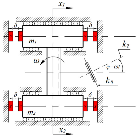
Figure 1. The Schematic representation of a system composed of two oscillators connected with periodically variable stiffness. (Color online).

The mechanical system consists of two masses $m_1$ and $m_2$, connected with a rectangular shaft. When an external excitation is applied, the shaft rotates with an angular frequency $\omega$ in the counterclockwise direction. As the shaft is rectangular in size and is rotating, the spring constants of the coupled system also vary periodically. While applying the external excitation in the system, the two masses $m_1$ and $m_2$ move back and forth on the hard surfaces. This movement is done by the real rolling bearings attached with the masses [27]. The resistance force $F_{\mathrm{Ri}}\left(\dot{x_i}\right)$ of the system is composed of two functions, one is viscous damping $C_i\dot{x_i}$ and another one is the force due to the dry friction. $x_1$ and $x_2$ are the displacements of the two masses $m_1$ and $m_2$ from the equilibrium positions. The inclusion of the four pairs of magnets with the identical polarities in the system creates the repulsive magnetic force $F_{\mathrm{Si}}\left(x_i\right)$, where $i=1,2$, acting on the two masses. Each pair of magnets have been placed at a fixed distance $\delta$. In our work, we keep varying the angular frequency $\omega$ of the system, keeping the remaining parameters fixed and observing the state variables’ dynamics under varying $\omega$ parameter conditions.

3. Mathematical Model

3.1. Dimensional Equations of the System

If we take all the components of the considered system to be ideal, the system can be described by a set of second order coupled ODEs, given by:

$$m_1{\ddot{x}}_1+F_{\mathrm{R}1}\left({\dot{x}}_1\right)+F_{\mathrm{S}1}\left(x_1\right)+K_{\mathrm{C}}\left(t\right)(x_1-x_2)=0$$

(1)

and,

$$m_2{\ddot{x}}_2+F_{\mathrm{R}2}\left({\dot{x}}_2\right)+F_{\mathrm{S}2}\left(x_2\right)+K_{\mathrm{C}}\left(t\right)(x_2-x_1)=0$$

(2)

where,

1

$F_{\mathrm{Ri}}\left({\dot{x}}_i\right)=C_i{\dot{x}}_i+\frac{T_i{\dot{x}}_i}{{\left({\dot{x}}_i^2+{ϵ}^2\right)}^{\frac{1}{2}}}$; $i=1,2$. $F_{\mathrm{Ri}}\left({\dot{x}}_i\right)$ is the resistance force of the bearings and the term $\frac{1}{{\left({\dot{x}}_i^2+{ϵ}^2\right)}^{\frac{1}{2}}}$ is the smooth approximation of the function sign(${\dot{x}}_i$).

2

$F_{\mathrm{Si}}\left(x_i\right)$ is the force due to the magnetic spring.

$F_{\mathrm{Si}}\left(x_i\right)=F_M(\delta -x_i)-F_M(\delta +x_i)$ = $F_{\mathrm{MO}}\left[\frac{1}{{\{1+d_1(\delta -x_i)\}}^4}-\frac{1}{{\{1+d_1(\delta +x_i)\}}^4}\right]$; $i=1,2$. The idea of the above formula is considered by the two assumptions: (i) the repulsive force between two magnets is defined by the simplest expression of the inverse square law, where the dipole expression has been considered. (ii) when $x_i$ = $\delta$, the first term of the $F_{\mathrm{Si}}\left({\dot{x}}_i\right)$ expression becomes the unity, when $x_i$ = $-\delta$, the second term becomes unity, and the expression $F_{\mathrm{Si}}\left({\dot{x}}_i\right)$ becomes negative value.

3

The stiffness coupling of the considered system, $K_{\mathrm{C}}\left(t\right)$ = $\left(\frac{K_1+K_2}{2}\right)+\left(\frac{K_1-K_2}{2}\right)cos\left(2{\omega }_{\mathrm{e}}t\right)$. It varies periodically having the linear frequency, $f=2·\frac{{\omega }_{\mathrm{e}}}{2\pi }$, where ${\omega }_{\mathrm{e}}$ is the angular frequency of oscillation.

The Equations (1) and (2) are the expressions in the dimensional form. Those equations will be useful to explain the system’s dynamics experimentally. For the numerical works, we have transformed those equations into non-dimensional forms. The development of the equations is given below.

3.2. Non-Dimensional Equations of the System

In order to transform the Equations (1) and (2) from the dimensional to the non-dimensional, we have introduced non-dimensional time as $\tau =2\pi f_{\mathrm{n}}t$. So, in the case of non-dimensional equations, the derivative has been done with respect to $\tau$, where $f_{\mathrm{n}}$ is the natural linear frequency of oscillation of the considered system, $f_{\mathrm{n}}=\frac{{\omega }_{\mathrm{n}}}{2\pi }$, and ${\omega }_{\mathrm{n}}=\sqrt{\frac{K_1}{m_1}}$.

Now, we introduce the expression of the non-dimensional frequency as, ${\omega }_{\mathrm{nd}}=\frac{{\omega }_{\mathrm{e}}}{{\omega }_{\mathrm{n}}}$. The non-dimensional state-variables as $y_{\mathrm{i}}=\frac{x_{\mathrm{i}}}{\delta }$; $i=1,2$.

${\dot{x}}_{\mathrm{i}}=\frac{d{x}_{\mathrm{i}}}{dt}$ = $\frac{d{x}_{\mathrm{i}}}{d\tau }·\frac{d\tau }{dt}$ = ${\omega }_{\mathrm{n}}\delta {\dot{y}}_{\mathrm{i}}$; similarly, ${\ddot{x}}_i$ = ${\omega }_{\mathrm{n}}^2\delta {\ddot{y}}_{\mathrm{i}}$.

So, from Equation (1),

$$\begin{array}{cc}\hfill & m_1{\omega }_{\mathrm{n}}^2\delta {\ddot{y}}_1+C_1{\omega }_{\mathrm{n}}\delta {\dot{y}}_1+\frac{T_1{\omega }_{\mathrm{n}}\delta {\dot{y}}_1}{{\omega }_{\mathrm{n}}\delta {\left\{{\dot{y}}_1^2+{\left(\frac{ϵ}{{\omega }_{\mathrm{n}}\delta }\right)}^2\right\}}^{\frac{1}{2}}}+F_{\mathrm{MO}}\left[\frac{1}{{\{1+d_1(\delta -\delta y_1)\}}^4}-\frac{1}{{\{1+d_1(\delta +\delta y_1)\}}^4}\right]\hfill \\ & +K_1\delta \left\{\left(\frac{1+\frac{K_2}{K_1}}{2}\right)+\left(\frac{1-\frac{K_2}{K_1}}{2}\right)\right\}cos\left(2{\omega }_{\mathrm{nd}}\tau \right)·(y_1-y_2)=0\hfill \end{array}$$

(3)

Dividing both sides by $m_1{\omega }_{\mathrm{n}}^2\delta$, we obtain

$$\begin{array}{cc}\hfill & {\ddot{y}}_1+\frac{C_1}{m_1{\omega }_{\mathrm{n}}}{\dot{y}}_1+\frac{\frac{T_1}{m_1{\omega }_{\mathrm{n}}^2\delta }{\dot{y}}_1}{{\omega }_{\mathrm{n}}\delta {\left({\dot{y}}_1^2+a_1^2\right)}^{\frac{1}{2}}}+\frac{F_{\mathrm{MO}}}{m_1{\omega }_{\mathrm{n}}^2\delta }\left[\frac{1}{{\{1+d_1\delta (1-y_1)\}}^4}-\frac{1}{{\{1+d_1\delta (1+y_1)\}}^4}\right]\hfill \\ & +\left(\frac{K_1\delta }{m_1{\omega }_{\mathrm{n}}^2\delta }\right)·\left(\frac{1+\beta }{2}\right)\left\{1+\left(\frac{1-\beta }{1+\beta }\right)\right\}cos\left(2{\omega }_{\mathrm{nd}}\tau \right)·(y_1-y_2)=0\hfill \end{array}$$

From the above equation, we can write,

$$\begin{array}{cc}\hfill & {\ddot{y}}_1+2{\zeta }_1{\dot{y}}_1+\frac{t_1{\dot{y}}_1}{{\omega }_{\mathrm{n}}\delta {\left({\dot{y}}_1^2+a_1^2\right)}^{\frac{1}{2}}}+b_1\left[\frac{1}{{\{1+D_1({\delta }_1-y_1)\}}^4}-\frac{1}{{\{1+D_1({\delta }_1+y_1)\}}^4}\right]\hfill \\ & +\delta \left(\frac{1+\beta }{2}\right)\left\{1+\left(\frac{1-\beta }{1+\beta }\right)\right\}cos\left(2{\omega }_{\mathrm{nd}}\tau \right)·(y_1-y_2)=0\hfill \end{array}$$

(4)

where, ${\zeta }_1=\frac{C_1}{2m_1{\omega }_{\mathrm{n}}}$, $t_1=\frac{T_1}{m_1{\omega }_{\mathrm{n}}^2\delta }$, $a_1=\frac{ϵ}{{\omega }_{\mathrm{n}}\delta }$, $b_1=\frac{F_{\mathrm{MO}}}{K_1\delta }$, $D_1=d_1\delta$, $\beta =\frac{K_2}{K_1}$, and ${\delta }_1=1$.

The Equation (4) is the non-dimensional form of the Equation (1).

Similarly, from the Equation (2), we get the non-dimensional form as

$$\begin{array}{cc}\hfill & {\ddot{y}}_2+2{\zeta }_2{\dot{y}}_2+\frac{t_2{\dot{y}}_2}{{\omega }_{\mathrm{n}}\delta {\left({\dot{y}}_2^2+a_1^2\right)}^{\frac{1}{2}}}+b_2\left[\frac{1}{{\{1+D_1({\delta }_1-y_2)\}}^4}-\frac{1}{{\{1+D_1({\delta }_1+y_2)\}}^4}\right]\hfill \\ & +\mu \left(\frac{1+\beta }{2}\right)\left\{1+\left(\frac{1-\beta }{1+\beta }\right)\right\}cos\left(2{\omega }_{\mathrm{nd}}\tau \right)·(y_2-y_1)=0\hfill \end{array}$$

(5)

where, ${\zeta }_2=\frac{C_2}{2m_2{\omega }_{\mathrm{n}}}$, $t_2=\frac{T_2}{m_2{\omega }_{\mathrm{n}}^2\delta }$, $\mu =\frac{m_1}{m_2}$, and $b_2=b_1\mu$.

4. Numerical Results

4.1. Behavior of the Dry-Friction and Resistance Force Terms

Figure 2 shows the evolution of the non-dimensional dry-friction terms (as written in the Equations (4) and (5)) with the variations of the non-dimensional velocities of the two masses $m_1$ and $m_2$ respectively. From the Figure 2a, it can be said that when the non-dimensional velocity (${\dot{y}}_1$) has the negative values, the dry-friction value reaches to a negative constant value, i.e., $-0.2413$. This is the value of the negative $t_1$. When the non-dimensional velocity has the positive values, the non-dimensional dry-friction term reaches the $0.2413$ value, equal to the value of $t_1$. Those values are well agreed with the definition of a dry-friction in mechanical systems. In the case of the Figure 2b, the same agreement holds for the evolution of the non-dimensional dry-friction term with the non-dimensional velocity (${\dot{y}}_2$) of the mass $m_2$. The dry-friction term reaches a constant value of $-0.288$ and $0.288$ when the non-dimensional velocity, ${\dot{y}}_2$, has the negative and positive values, respectively.

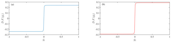
Figure 2. Evolution of the Dry-Friction terms with varying the (a) state-variable ${\dot{y}}_1$ of the first oscillator and (b) state-variable ${\dot{y}}_2$ of the second oscillator, respectively. In each figure, the x-axis is the non-dimensional velocities (i.e., state-variables ${\dot{y}}_1$ and ${\dot{y}}_2$) and the y-axis is the non-dimensional dry-friction terms. The parameter values are: $a_1=5.8548\times {10}^{-3}$, (a) ${\zeta }_1=0.0868$, (b) ${\zeta }_2=0.1036$. (Color online).

Figure 3 depicts the evolution of the resistance force terms $f_{\mathrm{R}1}\left({\dot{y}}_1\right)$ and $f_{\mathrm{R}2}\left({\dot{y}}_2\right)$ of the two oscillators with the variation of the velocities ${\dot{y}}_1$ and ${\dot{y}}_2$, respectively. From the Equations (4) and (5), we can say that the resistance force terms consist of two functions, one is linear damping, and another is the dry-friction term. So, when the velocity values continuously increase in a negative direction, the resistance force terms have linearly increasing slopes from the constant values in the negative direction along the y-axis with the negative directional variation of the velocities. The constant value is due to the dry-friction term, and the negative slope is due to the linear damping term. A similar thing happens when the velocity state variables are continuously increased in positive directions. The Figure 3a,b confirm the behavior of the resistance force terms, $f_{\mathrm{R}1}\left({\dot{y}}_1\right)$ and $f_{\mathrm{R}2}\left({\dot{y}}_2\right)$ with the variations of the velocity state-variables ${\dot{y}}_1$ and ${\dot{y}}_2$ respectively.

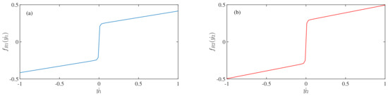
Figure 3. Plots of the resistance force terms $f_{\mathrm{R}1}\left({\dot{y}}_1\right)$ and $f_{\mathrm{R}2}\left({\dot{y}}_2\right)$ corresponding to the (a) state-variable ${\dot{y}}_1$ and (b) state-variable ${\dot{y}}_2$, respectively. In each figure, the x-axis is the non-dimensional velocities (i.e., state-variables ${\dot{y}}_1$ and ${\dot{y}}_2$) and the y-axis is the non-dimensional force due to the resistance term. The parameter values are: $a_1=5.8548\times {10}^{-3}$, (a) ${\zeta }_1=0.0868$, (b) ${\zeta }_2=0.1036$. (Color Online).

4.2. Behavior of Magnetic Spring Force Term

The non-dimensional magnetic spring force term can be expressed as-

$$f_{\mathrm{Si}}\left(y_i\right)=b_{\mathrm{i}}\left[\frac{1}{{\{1+D_1({\delta }_1-y_{\mathrm{i}})\}}^4}-\frac{1}{{\{1+D_1({\delta }_1+y_{\mathrm{i}})\}}^4}\right]$$

(6)

where, $\{i=1,2\}$.

If we plot $f_{\mathrm{S}1}\left(y_1\right)$ and $f_{\mathrm{S}2}\left(y_2\right)$ with the variation of the non-dimensional displacements $y_1$ and $y_2$, we obtain the Figure 4. Please note that, we have increased the non-dimensional displacements from $-{\delta }_1$ to $+{\delta }_1$ along the x-axis. The magnetic spring force value varies exponentially both in positive and negative directions of $y_i$, although at the neighborhood of 0, the curves of $f_{\mathrm{S}1}\left(y_1\right)$ and $f_{\mathrm{S}2}\left(y_2\right)$ are almost flat, parallel to the x-axis.

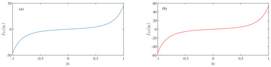
Figure 4. Plots of the magnetic spring force terms $f_{\mathrm{S}1}\left(y_1\right)$ and $f_{\mathrm{S}2}\left(y_2\right)$ with the variation of the (a) state-variable $y_1$ and (b) state-variable $y_2$, respectively. In each of the figures, the x-axis is the non-dimensional displacements (i.e., state-variables $y_1$ and $y_2$) and the y-axis is the non-dimensional magnetic spring force terms. The parameter values are: $D_1=1.5$, ${\delta }_1=1$, (a) $b_1=45.7143$, (b) $b_2=54.5737$. (Color Online).

The expression of the Equation (6) is complicated to implement in any physical system, like in an electronic circuit. So, we consider other functions that will yield the exact behaviors, but the expression is more straightforward.

$$f_{\mathrm{S}1}\left(y_1\right)=s_1{y}_1+s_2{y}_1^3$$

(7)

and,

$$f_{\mathrm{S}2}\left(y_2\right)=s_3{y}_2+s_4{y}_2^3$$

(8)

Now, if we compare the Equations (7) and (8) with the Equation (6), we can obtain the constant values of $s_1$, $s_2$, $s_3$, and $s_4$ as $5.476$, $40.0594$, $6.7078$, and $47.6527$ respectively.

The black curves in the Figure 5 show the function plot of the Equations (7) and (8). From the Figure 5a,b, we can say that the Equations (7) and (8) are well agreed with the Equation (6) and provide the same kind of behaviors.

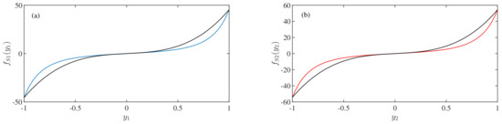
Figure 5. Comparison the magnetic spring force terms $f_{\mathrm{S}1}\left(y_1\right)$ and $f_{\mathrm{S}2}\left(y_2\right)$ obtained from the different expressions with the variation of the (a) state-variable $y_1$ and (b) state-variable $y_2$. The x-axes are the non-dimensional displacements (i.e., state-variables $y_1$ and $y_2$) and the y-axes are the non-dimensional magnetic spring force terms. The parameter values are: $D_1=1.5$, ${\delta }_1=1$, (a) $b_1=45.7143$, (b) $b_2=54.5737$. (Color Online).

4.3. Time-Series and Phase-Space Plots of the Considered System

Figure 6 shows the time-series waveforms of the mathematical Equations (4) and (5). These equations characterize the dynamics of the considered mechanical system. Here, we have varied the non-dimensional angular frequency, ${\omega }_{\mathrm{nd}}$, keeping the remaining parameter values fixed at ${\zeta }_1=0.0868$, ${\zeta }_2=0.1036$, $t_1=0.2413$, $t_2=0.288$, $b_1=45.7143$, $b_2=54.5737$, $a_1=5.8548\times {10}^{-3}$, $D_1=1.5$, $\beta =11.11$, $\mu =1.1938$, ${\delta }_1=1$. We have varied the ${\omega }_{\mathrm{nd}}$ in the range between $3.89$ to $4.1$. When the parameter ${\omega }_{\mathrm{nd}}$ is increased up to $3.89$ from the low value, the solutions of the state-variables, i.e., $y_1$, $y_2$, ${\dot{y}}_1$, and ${\dot{y}}_2$ give only the zero-fixed point solutions for any initial conditions. So, we get a straight line parallel to the time axis for each of the state-variables. Figure 6a shows the time series waveforms of the four state variables which signify the stable fixed point solutions. When ${\omega }_{\mathrm{nd}}$ is chosen to $4.00$, the period-1 time series waveforms come to an exist for all state-variables, which is shown in Figure 6b. When ${\omega }_{\mathrm{nd}}$ is at the value of $4.05$, the state-variables show the quasi-periodic nature in their time-series waveforms. Figure 6c shows the quasi-periodic time-series waveforms for four state-variables. The quasi-periodicity of the state-variables remains when ${\omega }_{\mathrm{nd}}$ is $4.093$. This is shown in Figure 6d. When ${\omega }_{\mathrm{nd}}$ is $4.098$, there is a chaotic attractor comes to an exist in the system. The corresponding time-series waveforms of the state-variables are shown in Figure 6e.

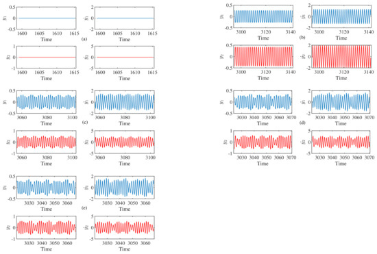
Figure 6. Time-Series waveforms of the considered system for different values of non-dimensional frequency, ${\omega }_{\mathrm{nd}}$. In each of the figure, x-axis is the non-dimensional time and the y-axis is the non-dimensional displacements, $y_1$ and $y_2$, and the non-dimensional velocities, ${\dot{y}}_1$, ${\dot{y}}_2$. The left and the right sides of the upper trace of each figure are the state-variables $y_1$ and ${\dot{y}}_1$ respectively. The left and the right sides of the lower trace of each figure are the state-variables $y_2$ and ${\dot{y}}_2$ respectively. (a) ${\omega }_{\mathrm{nd}}=3.89$, $y_1$ = $y_2$ = ${\dot{y}}_1$ = ${\dot{y}}_2$ = 0, i.e., fixed-point solutions, (b) ${\omega }_{\mathrm{nd}}=4.00$, Period-1 orbit, (c) ${\omega }_{\mathrm{nd}}=4.05$, quasi-periodic orbit, (d) ${\omega }_{\mathrm{nd}}=4.093$, quasi-periodic orbit, (e) ${\omega }_{\mathrm{nd}}=4.098$, chaotic orbit. The parameters are: ${\zeta }_1=0.0868$, ${\zeta }_2=0.1036$, $t_1=0.2413$, $t_2=0.288$, $b_1=45.7143$, $b_2=54.5737$, $a_1=5.8548\times {10}^{-3}$, $D_1=1.5$, $\beta =11.11$, $\mu =1.1938$, ${\delta }_1=1$. The initial condition is chosen to $(0.333,0,0,0)$ to obtain the time-series waveforms. (Color Online).

We have computed the phase spaces and the poincaré sections in the state-space to observe the actual periodicities of the system. In that case, we can distinctly observe different periodicities of the system while the parameter is varied. Figure 7 and Figure 8 show the phase-spaces and the poincaré sections of the coupled system for different values of ${\omega }_{\mathrm{nd}}$ respectively.

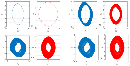
Figure 7. The phase portraits of the considered system for different values of ${\omega }_{\mathrm{nd}}$. x-axis is the non-dimensional displacements $y_1$, $y_2$ and the y-axis is the non-dimensional velocities ${\dot{y}}_1$, ${\dot{y}}_2$, respectively. The left and the right sides of each figure are the phase-portraits of each oscillator. (a) ${\omega }_{\mathrm{nd}}=4.00$, Period-1 orbit, (b) ${\omega }_{\mathrm{nd}}=4.05$, quasi-periodic orbit, (c) ${\omega }_{\mathrm{nd}}=4.093$, quasi-periodic orbit, (d) ${\omega }_{\mathrm{nd}}=4.098$, chaotic orbit. The parameters are: ${\zeta }_1=0.0868$, ${\zeta }_2=0.1036$, $t_1=0.2413$, $t_2=0.288$, $b_1=45.7143$, $b_2=54.5737$, $a_1=5.8548\times {10}^{-3}$, $D_1=1.5$, $\beta =11.11$, $\mu =1.1938$, ${\delta }_1=1$. The initial condition has been chosen at (0.333,0,0,0). (Color Online).

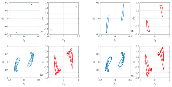
Figure 8. Poincaré sections of the considered system for different values of ${\omega }_{\mathrm{nd}}$. x-axis is the non-dimensional displacements $y_1$, $y_2$ and the y-axis is the non-dimensional velocities ${\dot{y}}_1$, ${\dot{y}}_2$, respectively. The left (blue color) and the right (red color) sides of each figure are the poincaré sections of each oscillator. (a) ${\omega }_{\mathrm{nd}}=4.00$, Period-1 orbit, (b) ${\omega }_{\mathrm{nd}}=4.05$, quasi-periodic orbit, (c) ${\omega }_{\mathrm{nd}}=4.093$, quasi-periodic orbit, (d) ${\omega }_{\mathrm{nd}}=4.098$, chaotic orbit. The parameters are: ${\zeta }_1=0.0868$, ${\zeta }_2=0.1036$, $t_1=0.2413$, $t_2=0.288$, $b_1=45.7143$, $b_2=54.5737$, $a_1=5.8548\times {10}^{-3}$, $D_1=1.5$, $\beta =11.11$, $\mu =1.1938$, ${\delta }_1=1$. The initial condition is chosen to $(0.333,0,0,0)$. (Color Online).

Figure 7 shows different phase space trajectories of the considered coupled system for different values of ${\omega }_{\mathrm{nd}}$. Figure 7a shows period-1 orbit in the phase space. The single loop confirms the period-1 in the phase space of the coupled system. When the parameter ${\omega }_{\mathrm{nd}}$ is increased to $4.05$, the system shows the quasi-periodic orbits in the phase-space diagram, which is shown in the Figure 7b. The quasi-periodic orbit with a different shape comes into existence in the parameter value of ${\omega }_{\mathrm{nd}}=4.093$, which is shown in the Figure 7c. When ${\omega }_{\mathrm{nd}}=4.098$, the orbit is chaotic. The chaotic attractor is shown in the Figure 7d.

It seems that the Figure 7c,d look like the same orbits. To distinguish between the quasi-periodicity and chaotic orbit, we have computed the poincaré sections, which are shown in the Figure 8.

The poincaré sections for different values of ${\omega }_{\mathrm{nd}}$ are shown in the Figure 8. As the system is a non-autonomous dynamical system, we need to observe the evolution of the state variables with the synchronism of the external periodic signal’s frequency. As the value of the frequency is $2f$, we shall observe the periodicity of the orbits in the interval of $\frac{T}{2}$. When the parameter value ${\omega }_{\mathrm{nd}}$ is $4.00$, the orbit is periodic. The dots in the Figure 8a confirm the period-1 of the coupled system. Please note that the two dots in the sampled state-space confirm the system’s symmetric nature. If we replace $y_1$ and $y_2$ by $-y_1$ and $-y_2$ in the Equations (4) and (5), we obtain the same expressions of the differential equations. It confirms the symmetricity of the equations of the coupled system. When ${\omega }_{\mathrm{nd}}$ is $4.05$, the system shows the quasi-periodic orbits. The single loop in the sampled state-space confirms the quasi-periodic nature of the system in that parameter range. When ${\omega }_{\mathrm{nd}}$ is increased more, at the value of $4.093$, the quasi-periodicity nature of the system exists. The poincaré section of the orbit in the phase space confirms this. In the Figure 8c, we can find that there are loops in the sampled state space. When ${\omega }_{\mathrm{nd}}$ is $4.098$, the orbit becomes chaotic. The corresponding poincaré section diagram is shown in the Figure 8d. Although it looks like loops in the sampled state space, the fuzzy dots in each loop make the orbit chaotic in the phase space.

When we vary the parameter ${\omega }_{\mathrm{nd}}$ from the low value to a higher value, we obtain different trajectories in the state space. To observe the whole dynamics of the system under the variation of the parameter value ${\omega }_{\mathrm{nd}}$, we now compute the bifurcation diagram. It is required to calculate the Lyapunov Exponents [28] and 0–1 test [29] to validate the existence of different dynamical behaviors in the system, such as different periodic orbits, quasi-periodic orbits, and chaotic orbits. We have computed maximal Lyapunov Exponents [30] only here to show all the periodicities, including chaos in the system in the parameter space.

4.4. Bifurcation Diagrams and the Corresponding Maximal Lyapunov Exponent

Figure 9a,b depict the numerically obtained bifurcation diagrams of the state-variables $y_1$ and $y_2$, respectively. The corresponding maximal Lyapunov exponent of the system is shown in Figure 9c. The Lyapunov exponent corresponding to the forcing phase was ignored here, since it is always equal to zero. During this calculation we have used the classical algorithm [30], where the re-normalization period was assumed to be equal to period of external excitation. For each value of the excitation angular frequency, the exponent was computed over time equal to 1000 normalization periods, after ignoring 100 initial excitation periods of transient motion.. We have chosen the bifurcation parameter value ${\omega }_{\mathrm{nd}}$ in the range between $3.89$ and $4.12$. When the parameter value is increased up to $3.905$ from a low value, we get only the fixed point attractor at $y_i^{*}=0$. When ${\omega }_{\mathrm{nd}}$ is varied more in the positive direction, the fixed point becomes unstable, and a period-1 orbit emerges by a supercritical Hopf bifurcation. While ${\omega }_{\mathrm{nd}}$ is increased more, the period-1 orbit persists up to the parameter value $4.023$. The corresponding Lyapunov exponent is the negative value, which is shown in the Figure 9c. At the point of $4.023$, a Neimark-Sacker bifurcation occurs, and the period-1 orbit loses its stability, and a quasi-periodic trajectory emerges. The maximal Lyapunov exponent reaches zero value at the bifurcation point $4.023$. The quasi-periodicity of the system persists up to the parameter value $4.09$. If one can notice carefully in the bifurcation diagram, there is a small chaotic window in-between the quasi-periodic orbit region in the parameter space between $4.05$ to $4.09$. The value of the ${\omega }_{\mathrm{nd}}$ corresponding to the chaotic regime is $4.074$. The maximal Lyapunov exponent shows the positive value where the system shows chaos. When the ${\omega }_{\mathrm{nd}}$ value is increased further from $4.09$, there is also a range of chaotic attractors with small periodic windows. The periodic window occurs at $4.094$. The fixed point solution starts to exist from the value of ${\omega }_{\mathrm{nd}}=4.10$. So, there is an interplay between quasi-periodicity and the chaotic orbits and chaotic orbits with periodic windows in the state variables in the bifurcation diagram. Due to the symmetric nature, the system has two bifurcation diagrams—one in the positive y-axis and another in the negative y-axis. We have chosen the initial condition as $[0.333,0,0,0]$.

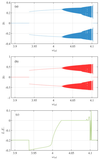
Figure 9. The bifurcation diagrams of the state variables $y_1$ and $y_2$, and the corresponding maximal lyapunov exponent of the system. (a) Bifurcation Diagram of $y_1$: The x-axis is the non-dimensional parameter ${\omega }_{\mathrm{nd}}$ and the y-axis is the sampled value of $y_1$, (b) Bifurcation Diagram of $y_2$: The x-axis is the non-dimensional parameter ${\omega }_{\mathrm{nd}}$ and the y-axis is the sampled value of $y_2$, (c) The maximum lyapunov exponent: The x-axis is the non-dimensional parameter ${\omega }_{\mathrm{nd}}$ and the y-axis is the lyapunov exponent. The parameters are: ${\zeta }_1=0.0868$, ${\zeta }_2=0.1036$, $t_1=0.2413$, $t_2=0.288$, $b_1=45.7143$, $b_2=54.5737$, $a_1=5.8548\times {10}^{-3}$, $D_1=1.5$, $\beta =11.11$, $\mu =1.1938$, ${\delta }_1=1$. The initial condition is considered as $(0.333,0,0,0)$. (Color Online).

4.5. Co-Existence of Two Attractors

Figure 10 shows all possible attractors in the bifurcation diagrams of the system when the state variable is $y_1$. The zero-fixed point exists because of the presence of the dry friction term. For the periodic orbit, the initial condition is chosen at $(0.333,0,0,0)$. The periodic orbits, along with the quasi-periodic and chaotic attractors, are shown in the figure by green color. The red line shows the co-existence of the zero-fixed point attractor for the initial condition at $(0,0,0,0)$.

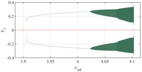
Figure 10. Co-existing attractors in the bifurcation diagram of $y_1$: The x-axis is the non-dimensional parameter ${\omega }_{\mathrm{nd}}$ and the y-axis is the sampled value of $y_1$. The parameters are: ${\zeta }_1=0.0868$, ${\zeta }_2=0.1036$, $t_1=0.2413$, $t_2=0.288$, $b_1=45.7143$, $b_2=54.5737$, $a_1=5.8548\times {10}^{-3}$, $D_1=1.5$, $\beta =11.11$, $\mu =1.1938$, ${\delta }_1=1$. (Color Online).

5. Equivalent Circuit of the Coupled Mechanical Oscillators

In order to validate the numerically predicted results, an equivalent circuit diagram of the coupled mechanical system is developed. To achieve this, we split the two-second order differential Equations (4) and (5) by two pairs of the first-order differential equations, which are shown below.

$$\begin{array}{cc}\hfill & {\dot{y}}_1=z_1\hfill \end{array}$$

(9a)

$$\begin{array}{cc}\hfill & {\dot{z}}_1=-\left[f_{\mathrm{R}1}\left(z_1\right)+f_{\mathrm{S}1}\left(y_1\right)+{\beta }_1\left(\tau \right)\right]\hfill \end{array}$$

(9b)

$$\begin{array}{cc}\hfill & {\dot{y}}_2=z_2\hfill \end{array}$$

(10a)

$$\begin{array}{cc}\hfill & {\dot{z}}_2=-\left[f_{\mathrm{R}2}\left(z_2\right)+f_{\mathrm{S}2}\left(y_2\right)+{\beta }_2\left(\tau \right)\right]\hfill \end{array}$$

(10b)

where,

1.

$f_{\mathrm{Ri}}\left(z_i\right)$ = $f_{\mathrm{LDi}}\left(z_i\right)$ + $f_{\mathrm{DFi}}\left(z_i\right)$ = $2{\zeta }_i{z}_i+\frac{t_i{z}_i}{{\left(z_i^2+a_1^2\right)}^{\frac{1}{2}}}$; $i=1,2$. $f_{\mathrm{Ri}}\left(z_i\right)$ is the non-dimensional resistance force of the bearings. $f_{\mathrm{LDi}}\left(z_i\right)$ is the linear damping force, and $f_{\mathrm{DFi}}\left(z_i\right)$ is the force due to the dry-friction. The values of ${\zeta }_1$, ${\zeta }_2$, $t_1$, $t_2$ and $a_1$ are $0.0868$, $0.1036$, $0.2413$, $0.2880$, and $5.8548\times {10}^{-3}$ respectively.

2.

$f_{\mathrm{Si}}\left(y_i\right)$ = $b_i\left[\frac{1}{{\{1+D_1({\delta }_1-y_i)\}}^4}-\frac{1}{{\{1+D_1({\delta }_1+y_i)\}}^4}\right]$; $i=1,2$., $f_{\mathrm{Si}}\left(y_i\right)$ is the non-dimensional force due to the magnetic spring. The values of $b_1$, $b_2$, $D_1$, and ${\delta }_1$ are $45.7143$, $54.5737$, $1.5$, and 1 respectively. To reduce the complexity of the equations, we have chosen the most straightforward expressions of the non-dimensional force due to the magnetic spring, which are in the Equations (7) and (8).

3.

The non-dimensional stiffness couplings of the considered system, ${\beta }_1\left(\tau \right)$ = $\left[\left(\frac{1+\beta }{2}\right)+\left(\frac{1-\beta }{2}\right)cos\left(2{\omega }_{\mathrm{nd}}\tau \right)\right](y_1-y_2)$ and ${\beta }_2\left(\tau \right)$ = $\mu \left[\left(\frac{1+\beta }{2}\right)+\left(\frac{1-\beta }{2}\right)cos\left(2{\omega }_{\mathrm{nd}}\tau \right)\right](y_2-y_1)$. The parameter values are $\beta =11.11$, $\mu =1.1938$. The non-dimensional angular frequency, ${\omega }_{\mathrm{nd}}$, will have to be varied in order to obtain the bifurcation diagram.

In order to draw the circuit diagram, the Equations (9) and (10) can be written as

$$\begin{array}{cc}\hfill & CR{\dot{y}}_1=-\left(\frac{R}{R}\right)(-z_1)\hfill \end{array}$$

(11a)

$$\begin{array}{cc}\hfill & CR{\dot{z}}_1=-\left(\frac{R}{R}\right)\left[f_{\mathrm{R}1}\left(z_1\right)+f_{\mathrm{S}1}\left(y_1\right)+{\beta }_1\left(\tau \right)\right]\hfill \end{array}$$

(11b)

$$\begin{array}{cc}\hfill & CR{\dot{y}}_2=-\left(\frac{R}{R}\right)(-z_2)\hfill \end{array}$$

(12a)

$$\begin{array}{cc}\hfill & CR{\dot{z}}_2=-\left(\frac{R}{R}\right)\left[f_{\mathrm{R}2}\left(z_2\right)+f_{\mathrm{S}2}\left(y_2\right)+{\beta }_2\left(\tau \right)\right]\hfill \end{array}$$

(12b)

First we have drawn the circuit diagrams of each of the components $f_{\mathrm{Ri}}\left(z_i\right)$, $f_{\mathrm{Si}}\left(y_i\right)$, ${\beta }_1\left(\tau \right)$, and ${\beta }_2\left(\tau \right)$.

5.1. Equivalent Circuit Diagram of the Dry-Friction Term $f_{\mathrm{DFi}}\left(z_i\right)$

The Figure 11 depicts the equivalent circuit diagram of the force due to the dry-friction $f_{\mathrm{DF}1}\left(z_1\right)$ of the first oscillator. $z_1$ is the applied input voltage. In order to obtain the expression of $f_{\mathrm{DF}1}\left(z_1\right)$, which is, $f_{\mathrm{DF}1}\left(z_1\right)=\frac{t_1{z}_1}{{\left(z_1^2+a_1^2\right)}^{\frac{1}{2}}}$, using analog circuit components, we first make the square of $z_1$. The multiplier $M1$ does this operation. So, the voltage $V_{15}$ in the Figure 11 is $z_1^2$. After that, the voltage $V_{15}$ is added with $q_1$ (i.e., $a_1^2$) using an inverting adder, $OA1$. So the output of $OA1$ is the $-\left(z_1^2+a_1^2\right)$. As, the output is negative, we now use a unity gain inverting op-amp $OA2$ to get the expression $\left(z_1^2+a_1^2\right)$.

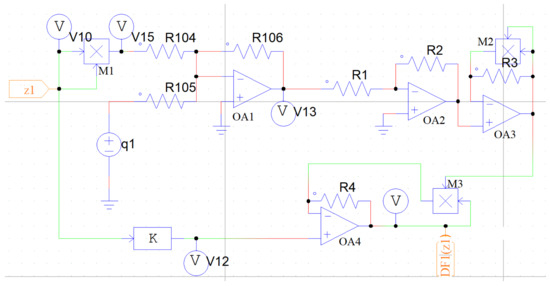
Figure 11. The equivalent circuit diagram of the force due to the dry-friction $f_{\mathrm{DF}1}\left(z_1\right)$. The resistance values are: $R_{104}$ = $R_{105}$ = $R_{106}$ = $R_1$ = $R_2$ = $R_3$ = $R_4$ = 100 k$\mathsf{\Omega }$, k = $0.2413$. $OA1$ to $OA4$ are the Op-Amps, $M_1$ to $M_3$ are the multipliers, $q_1$ is the dc voltage source with the value of $a_1^2$. K is the gain of a proportional block. (Color Online).

As the denominator of the second term of the expression of $f_{\mathrm{R}1}\left(z_1\right)$, is the square root of $\left(z_1^2+a_1^2\right)$, we use the op-amp $OA3$ to make the square-root of the output voltage of $OA2$, which is $V_{\mathrm{OA}2}$. For that, we have connected the $OA2$ op-amp’s output with the non-inverting input terminal of $OA3$. The output of the $OA3$ op-amp, $V_{\mathrm{OA}3}$ is connected to the inverting input of the $OA3$ op-amp through a multiplier $M2$. The output of $M2$ is the square of the output voltage of the op-amp $OA3$, i.e., $V_{\mathrm{OA}3}^2$. Due to the virtual connection concept of the two input terminals of an ideal op-amp, we can write, $V_{\mathrm{OA}3}^2$ = $V_{\mathrm{OA}2}$. Hence, $V_{\mathrm{OA}3}$ = $\sqrt{V_{\mathrm{OA}2}}$ = $\sqrt{\left(z_1^2+a_1^2\right)}$.

To get the numerator of the second term of $f_{\mathrm{R}1}\left(z_1\right)$, we have passed $z_1$ through a proportional block of gain $0.2413$ to achieve $0.2413z_1$ at the output of the proportional block.

The op-amp $OA4$ is used to make the ratio of the two signals. The output voltage of the proportional block is directly connected to the non-inverting input of the op-amp $OA4$. We have used the multiplier $M3$ to multiply the output of the op-amp $OA4$, i.e., $V_{\mathrm{OA}4}$ with the $V_{\mathrm{OA}3}$. So, the output of the multiplier $M3$ is $V_{\mathrm{OA}3}·V_{\mathrm{OA}4}$. This is connected to the inverting input of the op-amp $OA4$. Due to the virtual connection concept of an ideal op-amp, we can say that $0.2413z_1$ = $V_{\mathrm{OA}3}·V_{\mathrm{OA}4}$, which makes $V_{\mathrm{OA}4}$ = $\frac{0.2413z_1}{V_{\mathrm{OA}3}}$. So, the output of the op-amp $OA4$ provides the expression of the force due to the dry-friction, which is $f_{\mathrm{DF}1}\left(z_1\right)$ = $V_{\mathrm{OA}4}$ = $\frac{0.2413z_1}{\sqrt{\left(z_1^2+a_1^2\right)}}$.

Similarly, using the same logic, we have constructed the equivalent circuit diagram of the non-dimensional dry-friction force term of the second oscillator. For the second mechanical oscillator, the gain of the proportional block is chosen as $K=0.2880$. The circuit diagram is shown in the Figure 12. The output voltage of the op-amp OA8 provides the expression of $F_{\mathrm{DF}2}\left(z_2\right)$.

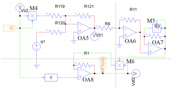
Figure 12. The equivalent circuit diagram of the force due to the dry-friction $f_{\mathrm{DF}2}\left(z_2\right)$. The resistance values are: $R_{119}$ = $R_{120}$ = $R_{121}$ = $R_9$ = $R_{1}1$ = $R_3$ = $R_1$ = 100 k$\mathsf{\Omega }$, k = $0.2413$. $OA4$ to $OA8$ are the four Op-Amps, $M_4$, $M_5$, and $M_6$ are the three multipliers, $q_1$ is the dc voltage source with the value of $a_1^2$. K is the gain of a proportional block. (Color Online).

5.2. Equivalent Circuit Diagram of the Magnetic Spring Force Term $f_{\mathrm{Si}}\left(y_i\right)$

Figure 13 expresses the equivalent circuit diagram of the non-dimensional magnetic spring force term $f_{\mathrm{S}1}\left(y_1\right)$ of the first oscillator. From the expression of $f_{\mathrm{S}1}\left(y_1\right)$ in the Equation (7), we can write the equivalent circuit equation as-

$$f_{\mathrm{S}1}\left(y_1\right)=-\left(\frac{R}{R_4}\right)(-y_1)-\left(\frac{R}{R_3}\right)(-y_1·y_1^2)$$

(13)

where, $\frac{R}{R_4}$ = $s_1$, $\frac{R}{R_3}$ = $s_2$, $y_1$ and $-y_1$ are the state-variables.

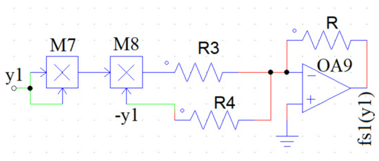
Figure 13. The equivalent circuit diagram of the force due to the magnetic spring $f_{\mathrm{S}1}\left(y_1\right)$. The resistance values are: $R_3$ = $2.50$ k$\mathsf{\Omega }$, $R_4$ = $18.26$ k$\mathsf{\Omega }$, $R=100$ k$\mathsf{\Omega }$. $OA9$ is the Op-Amp, $M_7$ and $M_8$ are the two multipliers. (Color Online).

The Equation (13) is implemented in the Figure 13. First, the input $y_1$ is squared using a multiplier $M_7$. Then the output of the multiplier $M_7$ is multiplied with $-y_1$ using another multiplier $M_8$ to achieve $-y_1^3$ at the output. We have added $-y_1^3$ and $-y_1$ using an inverting adder to obtain the expression of magnetic spring force term $f_{\mathrm{S}1}\left(y_1\right)$.

Similarly, using the same idea, we can make the circuit (as shown in the Figure 14) for the expression $f_{\mathrm{S}2}\left(y_2\right)$. In that case, $\frac{R}{R_{11}}$ = $s_3$, $\frac{R}{R_{12}}$ = $s_4$, $y_2$ and $-y_2$ are the state-variables used as the input.

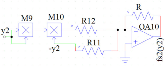
Figure 14. The equivalent circuit diagram of the force due to the magnetic spring $f_{\mathrm{S}2}\left(y_2\right)$. The resistance values are: $R_{11}$ = $14.91$ k$\mathsf{\Omega }$, $R_{12}$ = $2.1$ k$\mathsf{\Omega }$, $R=100$ k$\mathsf{\Omega }$. $OA10$ is the Op-Amp, $M_9$ and $M_{1}0$ are the two multipliers. (Color Online).

5.3. Equivalent Circuit Diagram of ${\beta }_i\left(\tau \right)$

From the Equation (9b), we can re-write the expression of the non-dimensional stiffness coupling of the first oscillator as ${\beta }_1\left(\tau \right)$ = $\left[\left(\frac{\beta +1}{2}\right)-\left(\frac{\beta -1}{2}\right)cos\left(2{\omega }_{\mathrm{nd}}\tau \right)\right](y_1-y_2)$.

If we insert the value of the $\beta =11.11$, we get, ${\beta }_1\left(\tau \right)$ = $(6.055-5.055cos\left(2{\omega }_{\mathrm{nd}}\tau \right))(y_1-y_2)$.

Similarly, from the Equation (10b), considering the value of $\mu$ as $1.1938$, we get, ${\beta }_2\left(\tau \right)$ = $(7.2284-6.0346cos\left(2{\omega }_{\mathrm{nd}}\tau \right))(y_2-y_1)$.

The Figure 15 is the corresponding circuit diagram of the term ${\beta }_1\left(\tau \right)$. From the expression of ${\beta }_1\left(\tau \right)$, first we implement the $(-5.055cos\left(2{\omega }_{\mathrm{nd}}\tau \right))$ term.

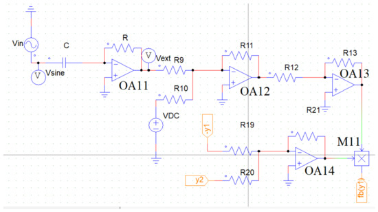
Figure 15. The equivalent circuit diagram of the non-dimensional spring force term ${\beta }_1\left(\tau \right)$. The resistance values are: R = $R_9$ = $R_{10}=R_{11}=R_{13}=R_{12}=R_{19}=R_{20}{R}_{21}=100$ k$\mathsf{\Omega }$. The capacitor $C=1$ nF. OA11, OA12, OA13, and OA14 are the four Op-Amps, $M_{1}1$ is the multiplier. $V_{\mathrm{in}}$ is the sine wave originating from a function generator. $V_{\mathrm{DC}}$ is a dc voltage source of value $6.055$ V. (Color Online).

In the Figure 15, $V_{\mathrm{in}}$ is a sine wave having an amplitude and frequency V and f, respectively. So, $V_{\mathrm{in}}$ can be expresses as, $V_{\mathrm{in}}=Vsin\left(2\pi ft\right)$. We pass this sine wave through a differentiator op-amp OA11. The output the differentiator will be $V_{\mathrm{ext}}$ = $-2\pi Vfcos\left(2\pi ft\right)$, which is equivalent to the expression $(-5.055cos\left(2{\omega }_{\mathrm{nd}}\tau \right))$. So, $-2\pi Vf$ = $-5.055$, which gives,

$$V=\frac{5.055}{2\pi f}$$

(14)

As, as the non-dimensional time can be expressed as, $\tau =\frac{t}{CR}$, we can write, $2{\omega }_{\mathrm{nd}}\tau$ = $2\pi ft$, which yields,

$$f=\frac{{\omega }_{\mathrm{nd}}}{\pi CR}$$

(15)

The output of the op-amp OA11, $V_{\mathrm{ext}}$, is added with a dc voltage, $V_{\mathrm{DC}}$ (having the value $6.055$) using an inverting adder op-amp OA12. The expression of the output becomes $-V_{\mathrm{DC}}-V_{\mathrm{ext}}$. This output will be in phase with $V_{\mathrm{ext}}$ after passing through a unity gain inverting op-amp OA13. So, the output of OA13 becomes $(6.055-5.055cos\left(2{\omega }_{\mathrm{nd}}\tau \right))$.

The op-amp OA14 adds the two inputs $-y_1$ and $y_2$ and gives the output in the form of $(y_1-y_2)$. The multiplier $M11$ multiplies the output of the two op-amps OA13 and OA14, and creates ${\beta }_1\left(\tau \right)$ as an output.

In order to make the equivalent circuit of the term ${\beta }_2\left(\tau \right)$, we have chosen the same approach. The only difference from ${\beta }_1\left(\tau \right)$ is that, an extra $\mu$ term is multiplied with the ${\beta }_1\left(\tau \right)$ term, and the sign of the two inputs are interchanged, i.e., $y_1$ and $-y_2$. The expression of the amplitude of the input ac sine wave will be,

$$V=\frac{6.0346}{2\pi f}$$

(16)

The expression of the linear frequency f will remain the same as calculated in the Equation (15). The circuit diagram is shown in Figure 16.

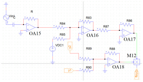
Figure 16. The equivalent circuit diagram of the non-dimensional spring force term ${\beta }_2\left(\tau \right)$. The resistance values are: R = $R_{84}$ = $R_{85}=R_{83}=R_{86}=R_{87}=R_{88}=R_{89}=R_{90}=100$ k$\mathsf{\Omega }$. The capacitor $C=1$ nF. OA15, OA16, OA17, and OA18 are the four Op-Amps, $M_{12}$ is the multiplier. $V_{\mathrm{in}1}$ is the sine wave. $V_{\mathrm{DC}1}$ is a dc voltage source of value $7.2284$ V. (Color Online).

Up to this, we have explained the electronic circuit analog of the forces due to the dry-friction, magnetic spring, and the non-dimensional springs, respectively of the coupled system. Now, we shall explain the main circuit diagram using the Equations (11) and (12).

Figure 17 depicts the equivalent circuit diagram of the considered coupled mechanical oscillators. The outputs of the op-amps OA20, OA24, OA26, OA30 are the four state-variables of the system, $y_1$, $z_1$, $y_2$, and $z_2$, respectively. DF1, DF2 are the boxes of the non-dimensional dry-friction force terms of the two oscillators. The circuits contained in the DF1 and DF2 are shown in the Figure 11 and Figure 12, respectively. Beta1(Tau) and Beta2(Tau) are the boxes containing the non-dimensional spring force terms of the two oscillators. The circuits inside the boxes are shown in the Figure 15 and Figure 16, respectively.

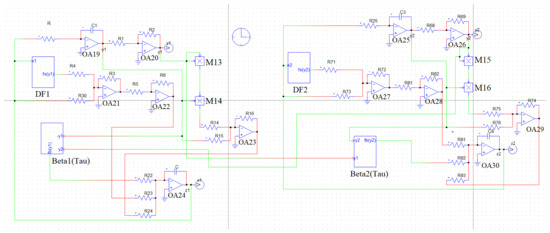
Figure 17. The analog circuit diagram of the considered mechanical system. The resistance values are: R = $R_1$ = $R_2$ = $R_3=R_4=R_5=R_6=R_{16}=R_{22}=R_{23}$ = $R_{24}=R_{25}=R_{68}=R_{69}=R_{71}=R_{72}=R_{74}=R_{81}=R_{82}=R_{91}=R_{92}=R_{93}$ = 100 k$\mathsf{\Omega }$, $R_{30}=576.04$ k$\mathsf{\Omega }$, $R_{73}=482.62$ k$\mathsf{\Omega }$, $R_{14}=2.50$ k$\mathsf{\Omega }$, $R_{15}=18.26$ k$\mathsf{\Omega }$, $R_{75}=2.1$ k$\mathsf{\Omega }$, $R_{76}=14.91$ k$\mathsf{\Omega }$. The capacitor values: $C=C_1=C_3=C_8=1$ nF. ‘OA’—series are the op-amps with different operations, $M_{13}$–$M_{16}$ are the multipliers. The initial capacitor voltage of $C_1$ is chosen at $0.333$ V, and the remaining capacitor initial voltages are kept at zero voltage. (Color Online).

OA19, OA20, M13, M14, and OA23 constitute the non-dimensional magnetic spring force term of the first mechanical oscillator which has been shown in detail in the Figure 13. Similarly, OA25, OA26, M15, M16, and OA29 constitute the non-dimensional magnetic spring force term of the second mechanical oscillator, which has also been shown in detail in the Figure 14.

The output voltage of the op-amp OA22 and OA28 are the forces due to the resistance. The values of the resistances $R_{30}$ and $R_{73}$ constitute the values of $2{\zeta }_1$ and $2{\zeta }_2$, respectively.

We have done the simulation of the circuit shown in Figure 16, using the PSIM 2.9 software. To simulate the circuit, we have chosen the time step value as ${10}^{-6}$ s, total time 5 s and have plotted the last 2 s only. We can perform this experiment in an actual electronic regime. Still, as already we have considered all the practical circuit components in the PSIM simulation, we think that this simulation will more or less support the experimental observations in the actual system.

In the next section, we have shown different time-series and phase-portraits by varying the parameter f, the linear frequency of the two ac signals used in the non-dimensional spring force term equivalent circuit. We have kept the other parameters fixed.

6. Results Obtained from Simulating the Circuit

In case of numerical results, we mainly observed the dynamical behaviors of the considered system under varying parameter, ${\omega }_{\mathrm{nd}}$. In the case of electronic circuit implementation, we have observed the phase portraits for different ${\omega }_{\mathrm{nd}}$. From the Equation (15), we can say that the linear frequency f of the applied sine wave is dependent on the non-dimensional angular frequency ${\omega }_{\mathrm{nd}}$ of the considered mechanical system. So, to validate the numerical predictions using the electronic circuit set-up, we have varied f to obtain different ${\omega }_{\mathrm{nd}}$.

When, ${\omega }_{\mathrm{nd}}=3.89$, from the Equation (15), the expression of the linear frequency f is $12.382$ kHz, where $C=1$ nF, and $R=100$ k$\mathsf{\Omega }$. Figure 18 shows the time-series waveforms of the four state-variables of the analog electronic circuit of the considered coupled mechanical system. The waveforms are straight lines parallel to the x-axis, implying that the circuit has a zero-fixed point solution. We observed the same time-series waveforms in the case of numerical simulation as shown in the Figure 6a. The zero fixed point exists for any initial conditions. The corresponding amplitudes of the applied ac sine waves of the first and second oscillators equivalent circuits are $0.6497$ V and $0.7756$ V, respectively. The voltages have been calculated using the Equations (14) and (16).

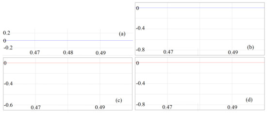
Figure 18. Time-series waveforms of the four state-variables obtained from the circuit simulation for ${\omega }_{\mathrm{nd}}=3.89$. For each figure, x-axis is the time in sec and the y-axis is the values of $y_1$, $y_2$, $z_1$, and $z_2$, respectively in V. (a) Time-series waveform of $z_1$, (b) Time-series waveform of $y_2$, (c) Time-series waveform of $y_1$, and (d) Time-series waveform of $z_2$. The frequency of the sine wave generator is $12.382$ kHz. The initial condition has been chosen at (0.333,0,0,0) to obtain the time-series waveforms. (Color Online).

When ${\omega }_{\mathrm{nd}}=4.00$, the Figure 19 shows the corresponding phase space diagrams of the circuit shown in the Figure 17. From the Equation (15), $f=12.732$ kHz. The single loop in the phase space confirms that the orbit is periodic of an order 1. The same thing we predicted in the numerical result in the Figure 7a. Using the Equations (14) and (16), we can calculate the values of the amplitudes of the applied ac sine waves. The amplitudes of $V_{\mathrm{in}}$ and $V_{\mathrm{in}1}$ for the first and second oscillators are $0.6319$ V and $0.7543$ V, respectively. Please note that we have chosen the initial condition as $(0.333,0,0,0)$. Suppose we choose the initial condition as $(0,0,0,0)$. In that case, we obtain the zero fixed point trajectories for all the state variables, which confirm that the system has a co-existence of two attractors, one is a zero fixed point attractor, and another one is a period-1 orbit. The same agreement is shown in the numerically obtained bifurcation diagram in the Figure 10, where one can see that the two attractors coexist in the bifurcation diagrams. The red color is the fixed point attractor for the initial conditions $(0,0,0,0)$, and the green color is the different periodic orbits depending upon the different ${\omega }_{\mathrm{nd}}$ values. For the electronic circuit, the initial condition values have been chosen as the initial capacitor voltages in the circuit, as shown in the Figure 17.

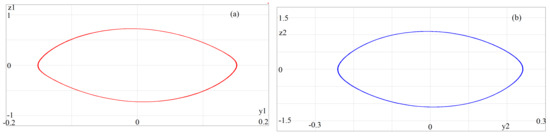
Figure 19. Phase-space diagrams of the circuit when $f=12.732$ kHz. The corresponding value of ${\omega }_{\mathrm{nd}}$ is $4.00$. (a) x-axis is the voltage of $y_1$ in V and y-axis is the voltage of $z_1$ in V, (b) x-axis is the voltage of $y_2$ in V and y-axis is the voltage of $z_2$ in V. The initial condition has been chosen at $(0.333,0,0,0)$ to obtain the phase portraits. (Color Online).

When ${\omega }_{\mathrm{nd}}$ is $4.05$, the corresponding value of the linear frequency f is calculated using Equation (15) as $12.892$ kHz. The phase space diagram of the equivalent circuit is shown in Figure 20. The amplitudes of the two sine waves $V_{\mathrm{in}}$ and $V_{\mathrm{in}1}$, used at the circuit diagrams Figure 15 and Figure 16 are $0.6241$ V and $0.7450$ V, respectively. The phase portraits obtained from the circuit diagram agree with the numerical prediction of the phase space diagrams for ${\omega }_{\mathrm{nd}}=4.05$ as shown in the Figure 7b. The orbit is quasi-periodic in nature which is confirmed from the Figure 8b. Here also, the initial condition is $(0.333,0,0,0)$. If we change the initial condition $(0,0,0,0)$, we only observe the zero fixed-point solutions.

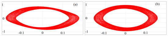
Figure 20. Phase-space diagrams of the circuit when $f=12.892$ kHz. The corresponding ${\omega }_{\mathrm{nd}}=4.05$. (a) x-axis is the voltage of $y_1$ in V and y-axis is the voltage of $z_1$, (b) x-axis is the voltage of $y_2$ in V and y-axis is the voltage of $z_2$ in V. The initial condition has been chosen at (0.333,0,0,0) to obtain the phase portraits. (Color Online).

When ${\omega }_{\mathrm{nd}}$ is equal to the value $4.098$, the corresponding linear frequency f of the circuit is $13.044$ kHz. The phase portraits of the circuit at this frequency are shown in the Figure 21. The phase portraits are chaotic in nature. The numerical phase portraits which we obtained in the Figure 7d are the same as the phase portraits obtained from the circuit diagram. Please note that the amplitudes $V_{\mathrm{in}}$ and $V_{\mathrm{in}1}$ of the ac sine waves for the oscillator 1 and oscillator 2 are $0.6168$ V and $0.7363$ V, respectively. The coexisting attractors are validated in this case also.

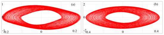
Figure 21. Phase-space diagrams of the circuit when $f=13.044$ kHz. The corresponding ${\omega }_{\mathrm{nd}}=4.098$. (a) x-axis is the voltage of $y_1$ in V and y-axis is the voltage of $z_1$ in V, (b) x-axis is the voltage of $y_2$ in V and y-axis is the voltage of $z_2$ in V. The initial condition has been chosen at (0.333,0,0,0) to obtain the phase portraits. (Color Online).

So, the circuit in the Figure 17 can be used as an equivalent electronic circuit of the considered mechanical system. The waveforms and the phase portraits of the circuit validate the numerical predictions of the system. If one can notice carefully, the phase portraits obtained from the numerical simulation and obtained from the circuit have different scaling values, although the shapes are the same. These things have happened because the differential equations are non-dimensionalized, and the circuits equations are dimensional. Also, the parameter values of the two cases are nearly equal, not the same. But the periodicities of the phase space trajectories are the same.

7. Conclusions

This paper shows the electronic circuit equivalence of coupled mechanical oscillators subjected to the influence of resistance magnetic spring forces. We have calculated the non-dimensional equations of the considered system. The numerical results obtained from these equations show some typical dynamics, such as the transitions from a fixed point to the periodic, quasiperiodic, and chaotic orbits, while varying the bifurcation parameter in one direction. We have constructed the electronic circuits of the force due to the dry-friction, magnetic spring force, and parametrically excited spring constant force. These circuits are straightforward and more convenient to use in future works. We have validated the numerical results by showing the time-series and phase-space diagrams of the equivalent analog circuit of the system.

We may perform the actual experiment in the breadboard, but the circuit diagram in the PSIM software is well demonstrated. We have chosen the op-amps, multipliers, etc., to design the circuit. So, the circuit diagram simulated in software supports the actual experiment.

References

- Awrejcewicz, J.; Lamarque, C.H. Bifurcation and Chaos in Nonsmooth Mechanical Systems; World Scientific: Singapore, 2003; Volume 45. [Google Scholar]
- Sidorets, V.; Pentegov, I. Deterministic Chaos in Nonlinear Circuits with Electric Arc; International Association Welding: Kyiv, Ukraine, 2013. [Google Scholar]
- Witkowski, K.; Kudra, G.; Skurativskyi, S.; Wasilewski, G.; Awrejcewicz, J. Modeling and dynamics analysis of a forced two-degree-of-freedom mechanical oscillator with magnetic springs. Mech. Syst. Signal Process. 2021, 148, 107138. [Google Scholar] [CrossRef]
- Kudra, G.; Witkowski, K.; Seth, S.; Polczyński, K.; Awrejcewicz, J. Parametric Vibrations of a System of Oscillators Connected with Periodically Variable Stiffness. In Proceedings of the DSTA-2021 Conference Books–Abstracts (16th International Conference: Dynamical Systems Theory and Applications DSTA 2021 ABSTRACTS), Łódź, Poland, 16–19 December 2021; Awrejcewicz, J., Ka´zmierczak, M., Olejnik, P., Mrozowski, J., Eds.; Wydawnictwo Politechniki Łódzkiej: Łódź, Poland. ISBN 978-83-66741-20-1. [Google Scholar] [CrossRef]
- Lu, Z.Q.; Ding, H.; Chen, L.Q. Resonance response interaction without internal resonance in vibratory energy harvesting. Mech. Syst. Signal Process. 2019, 121, 767–776. [Google Scholar] [CrossRef]
- Wojna, M.; Wijata, A.; Wasilewski, G.; Awrejcewicz, J. Numerical and experimental study of a double physical pendulum with magnetic interaction. J. Sound Vib. 2018, 430, 214–230. [Google Scholar] [CrossRef]
- Chiacchiari, S.; Romeo, F.; McFarland, D.M.; Bergman, L.A.; Vakakis, A.F. Vibration energy harvesting from impulsive excitations via a bistable nonlinear attachment. Int. J. Non-Linear Mech. 2017, 94, 84–97. [Google Scholar] [CrossRef]
- Chiacchiari, S.; Romeo, F.; McFarland, D.M.; Bergman, L.A.; Vakakis, A.F. Vibration energy harvesting from impulsive excitations via a bistable nonlinear attachment—Experimental study. Mech. Syst. Signal Process. 2019, 125, 185–201. [Google Scholar] [CrossRef]
- Witkowski, K.; Kudra, G.; Wasilewski, G.; Awrejcewicz, J. Modelling and experimental validation of 1-degree-of-freedom impacting oscillator. Proc. Inst. Mech. Eng. Part J. Syst. Control Eng. 2019, 233, 418–430. [Google Scholar] [CrossRef]
- Sanches, L.; Michon, G.; Berlioz, A.; Alazard, D. Response and instability prediction of helicopter dynamics on the ground. Int. J. Non-Linear Mech. 2014, 65, 213–225. [Google Scholar] [CrossRef]
- Danylenko, V.; Skurativskyi, S. Peculiarities of wave fields in nonlocal media. arXiv 2015, arXiv:1503.01351. [Google Scholar]
- Olejnik, P.; Awrejcewicz, J. Coupled oscillators in identification of nonlinear damping of a real parametric pendulum. Mech. Syst. Signal Process. 2018, 98, 91–107. [Google Scholar] [CrossRef]
- Skurativskyi, S.; Kudra, G.; Witkowski, K.; Awrejcewicz, J. Bifurcation phenomena and statistical regularities in dynamics of forced impacting oscillator. Nonlinear Dyn. 2019, 98, 1795–1806. [Google Scholar] [CrossRef] [Green Version]
- Ing, J.; Pavlovskaia, E.; Wiercigroch, M.; Banerjee, S. Bifurcation analysis of an impact oscillator with a one-sided elastic constraint near grazing. Phys. D Nonlinear Phenom. 2010, 239, 312–321. [Google Scholar] [CrossRef]
- Nguyen, H.T.; Genov, D.; Bardaweel, H. Mono-stable and bi-stable magnetic spring based vibration energy harvesting systems subject to harmonic excitation: Dynamic modeling and experimental verification. Mech. Syst. Signal Process. 2019, 134, 106361. [Google Scholar] [CrossRef]
- Afsharfard, A. Application of nonlinear magnetic vibro-impact vibration suppressor and energy harvester. Mech. Syst. Signal Process. 2018, 98, 371–381. [Google Scholar] [CrossRef]
- Novak, M.; Cernohorsky, J.; Kosek, M. Simple electro-mechanical model of magnetic spring realized from FeNdB permanent magnets. Procedia Eng. 2012, 48, 469–478. [Google Scholar] [CrossRef] [Green Version]
- Seth, S.; Banerjee, S. Electronic circuit equivalent of a mechanical impacting system. Nonlinear Dyn. 2020, 99, 3113–3121. [Google Scholar] [CrossRef]
- Skilling, H. An Electric Analog of Friction For Solution of Mechanical Systems Such as the Torsional-Vibration Damper. Trans. Am. Inst. Electr. Eng. 1931, 50, 1155–1158. [Google Scholar] [CrossRef]
- Berthet, R.; Petrosyan, A.; Roman, B. An analog experiment of the parametric instability. Am. J. Phys. 2002, 70, 744–749. [Google Scholar] [CrossRef] [Green Version]
- Jezierski, E. On electrical analogues of mechanical systems and their using in analysis of robot dynamics. In Robot Motion and Control; Springer: Berlin/Heidelberg, Germany, 2006; pp. 391–404. [Google Scholar]
- Kacar, S.; Wei, Z.; Akgul, A.; Aricioglu, B. A novel 4D chaotic system based on two degrees of freedom nonlinear mechanical system. Zeitschrift für Naturforschung A 2018, 73, 595–607. [Google Scholar] [CrossRef]
- López-Martínez, J.; Martínez, J.C.; García-Vallejo, D.; Alcayde, A.; Montoya, F.G. A new electromechanical analogy approach based on electrostatic coupling for vertical dynamic analysis of planar vehicle models. IEEE Access 2021, 9, 119492–119502. [Google Scholar] [CrossRef]
- Nishimori, Y.; Ooiso, H.; Mochizuki, S.; Fujiwara, N.; Tsuchiya, T.; Hashiguchi, G. A multiple degrees of freedom equivalent circuit for a comb-drive actuator. Jpn. J. Appl. Phys. 2009, 48, 124504. [Google Scholar] [CrossRef]
- Chang, F.; Wang, Z.; Tao, Y. Circuit simulation of two-degree-of-freedom unilateral impact dynamics system with gap. J. Phys. Conf. Ser. 2021, 1827, 012002. [Google Scholar] [CrossRef]
- Xu, Q.; Fan, W.; Luo, Y.; Wang, S.; Jiang, H. Nonlinear effect of forced harmonic oscillator subject to sliding friction and simulation by a simple nonlinear circuit. Am. J. Phys. 2019, 87, 116–124. [Google Scholar] [CrossRef]
- Awrejcewicz, J. Ordinary Differential Equations and Mechanical Systems; Springer: Berlin/Heidelberg, Germany, 2014. [Google Scholar]
- Xu, Q.; Zhu, D. FPGA-based experimental validations of electrical activities in two adjacent FitzHugh–Nagumo neurons coupled by memristive electromagnetic induction. IETE Tech. Rev. 2021, 38, 563–577. [Google Scholar] [CrossRef]
- Savi, M.A.; Pereira-Pinto, F.H.I.; Viola, F.M.; de Paula, A.S.; Bernardini, D.; Litak, G.; Rega, G. Using 0–1 test to diagnose chaos on shape memory alloy dynamical systems. Chaos Solitons Fractals 2017, 103, 307–324. [Google Scholar] [CrossRef]
- Wolf, A.; Swift, J.B.; Swinney, H.L.; Vastano, J.A. Determining Lyapunov exponents from a time series. Phys. D Nonlinear Phenom. 1985, 16, 285–317. [Google Scholar] [CrossRef] [Green Version]
Publisher’s Note: MDPI stays neutral with regard to jurisdictional claims in published maps and institutional affiliations. |
© 2022 by the authors. Licensee MDPI, Basel, Switzerland. This article is an open access article distributed under the terms and conditions of the Creative Commons Attribution (CC BY) license (https://creativecommons.org/licenses/by/4.0/).