Abstract
Environmental noise has become one of the principal health risks for urban dwellers and road traffic noise (RTN) is considered to be the main source of these adverse effects. To address this problem, strategic noise maps and corresponding action plans have been developed throughout Europe in recent years in response to the European Noise Directive 2002/49/EC (END), especially in populated cities. Recently, wireless acoustic sensor networks (WASNs) have started to serve as an alternative to static noise maps to monitor urban areas by gathering environmental noise data in real time. Several studies have analysed and categorized the different acoustic environments described in the END (e.g., traffic, industrial, leisure, etc.). However, most of them have only considered the dynamic evolution of the A-weighted equivalent noise levels over different periods of time. In order to focus on the analysis of RTN solely, this paper introduces a clustering methodology to analyse and group spectro-temporal profiles of RTN collected simultaneously across an area of interest. The experiments were conducted on two acoustic databases collected during a weekday and a weekend day through WASNs deployed in the pilot areas of the LIFE+ DYNAMAP project. The results obtained show that the clustering of RTN, based on its spectro-temporal patterns, yields different solutions on weekdays and at weekends in both environments, being larger than those found in the suburban environment and lower than the number of clusters in the urban scenario.
1. Introduction
Environmental noise has become one of the major pollutants in urban areas in recent years, having important negative effects on the quality of life of citizens [1,2]. In particular, the sustained increase in the number of urban dwellers has aggravated the problem of traffic noise, the main noise source of noise pollution in urban areas, which has serious consequences for the health of their inhabitants [3]. The European competent authorities reacted to this problem by developing the European Noise Directive 2002/49/EC (END) [4], and the subsequent strategic noise mapping assessment for its homogeneous application across Europe, denoted as CNOSSOS-EU [5]. The main goal of these regulations is to address the effects of environmental noise by requiring European member states to determine noise exposure, inform affected citizens and provide support to competent authorities to prevent and reduce environmental noise if required.
For this purpose, both noise maps and action plans have to be developed every five years for large agglomerations, according to the END legislation. Recently, the development of wireless acoustic sensor networks (WASNs) has provided information about environmental noise in real-time through low-cost multi-sensor networks deployed in smart cities (see [6] and references herein), improving the amount of data collected and available for the competent authorities. In this context, the LIFE+ DYNAMAP project [7] has developed a WASN-based dynamic noise mapping system to represent the acoustic impact of road infrastructures in real-time in two pilot areas [8,9]: one in the city of Milan as an urban area, and another on the outskirts of Rome as a suburban environment. Specifically, the urban WASN is composed of 24 acoustic nodes installed in different façades of public buildings across District 9 of Milan [10], while the suburban WASN is composed of 19 acoustic sensing nodes placed in the portals of the A90 motorway surrounding Rome [11].
For the proper computation of the equivalent noise levels () of road infrastructures, acoustic events unrelated to regular road traffic noise (RTN), (considered as those which come from from vehicles engines and the contact between their tyres and the pavement [7]), should be removed automatically to avoid biasing the RTN map generation. These events are denoted as anomalous noise events (ANEs) within the DYNAMAP project, and represent, for instance, trains, airplanes, sirens, horns, speech, doors, works, etc. To this end, an anomalous noise events detector (ANED) has been designed as a two-class classifier (ANE vs. RTN) using mel-frequency cepstral coefficients (MFCC) [12] and Gaussian mixture models, and has been implemented in the low-cost sensors running locally in real-time [13,14]. In order to train the ANED algorithm properly, several previous studies have focused on the collection, characterization and impact analysis of ANEs in the A-weighted environmental noise levels () computation (see e.g., [10,11,15]). However, much less attention has been paid to the majority class, that is, RTN, which represents around 90% of the collected data [15], which is also relevant, since spectral components and evolution of the road traffic noise of each specific location may also affect the performance of the ANED algorithm.
Several investigations have addressed the study of the similarities and differences of acoustic environments by means of clustering techniques, using data collected through WASNs. Most of them consider values computed, using several window spans, depending on the goal of each analysis, in the deployed sensors, as well as their temporal evolution during the day and on different days of the week. Among them, it is worth mentioning that several works have analysed Milan’s DYNAMAP urban environment to cluster that neighborhood through different approaches based on measurements. In [16], the presence of acoustic events is included in the analysis, by considering their impact merged with RTN levels through the intermittency ratio (IR). Other studies, such as [17,18] also consider curves with different analysis window sizes, together with other parameters, such as traffic speed data, to complement the equivalent noise levels and complete the classification of the monitored acoustic environments. However, these studies focus on high-level features (e.g., and IR) to analyse the acoustic environments of interest.
As an alternative to the categorization of acoustic environments based on their spectro-temporal behaviour, in [19], a preliminary proposal was described through the analysis of WASN-based raw acoustic data. The research showed the viability of the proposal, as well as the potential existence of two clusters in the urban pilot area of the DYNAMAP project. However, this conclusion was tentative as it was obtained through a straightforward visual inspection. Later, in [20], a further analysis was conducted by means of selecting two representative locations from each pilot area (Rome and Milan) on both weekdays and weekend days [21]. The analysis paid special attention to the low frequency range, which contains the main frequency components of RTN, as well as the sensor locations and day and night characteristics. The results showed a high dependence on the analysed environment and encouraged the authors to extend the study by considering all the sensors of both WASNs to characterize the spectro-temporal behaviour of the RTN across all the available locations.
Following the authors’ previous studies [19,20], this article introduces an analysis and clustering methodology to group road traffic noise spectro-temporal profiles, which are simultaneously collected across an area of interest during a given period of time. The approach, which is designed to determine the optimal number of clusters, as well as to interpret the results through expert-based post-processing, is evaluated using around 250 h of RTN-labelled data from the two pilot areas of the DYNAMAP project that were collected during a weekday and a weekend day.
The remaining sections of the paper are organized as follows. Section 2 describes the most relevant studies related to the clustering of acoustic environments. Section 3 describes the proposed analysis and clustering methodology on the spectro-temporal distributions of road traffic noise collected in different locations of an area of interest simultaneously, Next, Section 4 describes the experiments conducted, as well as the results obtained for the data collected from the urban and suburban pilot areas of the DYNAMAP project, during a weekday and a weekend day. Finally, Section 5 and Section 6 discuss the results obtained and present the conclusions of this research and several future research lines, respectively.
2. Related Work
In recent years, progress has been made in the deployment of different acoustic sensor networks designed for noise monitoring, especially in urban areas, where traffic noise is one of the main sources of annoyance described in the END [4]. The observation of the noise measured in each of the stations can lead to the classification of their locations, according to the measured level of noise, but also according to other urban parameters, such as the type of street, or the intensity of traffic measured or estimated by the municipalities.
Several studies can be found in the literature on the cluster analysis of urban acoustic environments. In [17], the authors introduced a clustering approach based on the k-means algorithm, considering yearly acoustic indexes, such as , and , as well as the standard deviation of . The sensor network under test was the Barcelona Noise Monitoring Network [22], which also measured noise levels with the final goal of the identification of several acoustic environments across the city. The results showed that the obtained clusters have a geographical meaning, as they correspond to locations close to high traffic roads, residential areas or leisure areas, respectively. Other studies, as [18], start with an approximation of road classification based on the road design and the traffic speed data. Subsequently, the equivalent noise levels of all the roads is included in the clustering. The final goal of the study conducted in Foshan (China) was to predict the equivalent noise level from vehicles’ speed and road design information. In [23], the authors propose a method to draw a spatio-temporal distribution of the noise levels in the city with two variables, the traffic density and the traffic speed, as well as spatio-temporal characteristics derived from the geography of the deployed network. The goal of the study was to evaluate the noise distributions corresponding to several periods by efficient algorithms of prediction with an acceptable accuracy.
The Milan pilot of the DYNAMAP project was widely analysed in terms of clustering the noise levels in the different sensor locations, in order to optimize the spatial distribution of noise monitoring stations. Preliminary studies described in [24,25] introduced a first statistical approach to the categorization of Milan’s District 9 roads, based on the clustering of 14-hourly , with the aim of progressing further in the classification than the information given by the legislative road categorization. Moreover, in [26], the authors describe another statistical clustering approach, where the roads having similar flow conditions—and hence similar noise trends due to road traffic—are grouped together, based on an extensive measurement campaign. The authors conclude that two clusters describe the roads in Milan more efficiently than the road categorisation used by the administration. More recent research in the same urban environment has widened the study to use up to 90 sensor locations to represent noise events The proposal was to cluster the sensors by means of the similarities among them. The data used to evaluate the clustering were the equivalent level and the intermittency ratio (IR), which is a metric that reflects the short-time variations of noise exposure [27], of all the sensor locations, the resulting clusters being highly related to the average day-time hourly traffic flow of vehicles. The authors of [28] managed to improve the accuracy of the noise map generation by means of the information given by each and every sensor location, considering the cluster to which each sensor belonged.
3. Analysis and Clustering Methodology
This section describes the methodology followed to analyse and group RTN data collected simultaneously from different measurement locations across a given area. The approach focused on investigating how many different acoustic environments, in terms of RTN, could be distinguished in the area of interest, e.g., a city district or a neighbourhood, based on the spectro-temporal analysis of real acoustic data gathered in that area. In order to focus on RTN, other noise sources, such as trains, airplanes, horns, sirens, birdsongs, dogs barking, works, people, rain, etc., should be removed beforehand to avoid any potential bias due to their occasional presence in the clustering and analysis of RTN distributions.
Figure 1 shows the block diagram of the proposed clustering methodology. First, acoustic data are gathered from locations simultaneously (e.g., from a WASN of sensors) of a given acoustic environment. The analysis considers a labelled acoustic database as input, which includes both the simultaneous collection of audio recordings for the period of interest (e.g., one day) together with the corresponding RTN labels. Next, the acoustic data are pre-processed before conducting the subsequent spectro-temporal analyses of RTN. To that effect, the audio passages of interest are selected from the sensed periods, considering if they sufficiently representative in terms of the presence of RTN. As a result, some sensed locations can be discarded (e.g., due to particular technical problems), being , the final number of locations considered for the subsequent analyses.
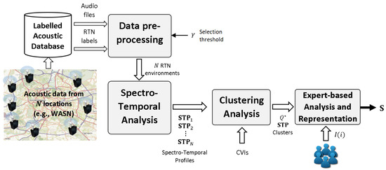
Figure 1.
Block diagram of the clustering and analysis methodology of RTN acoustic environments from the data collected from N locations simultaneously.
After conducting the spectro-temporal analysis of the acoustic data for each location considered, the obtained spectro-temporal profiles (STPs) are input into the clustering analysis to automatically obtain a set of STP groups based on the computation of a set of cluster validity indices (CVIs) that drive the selection of the optimal number of STP clusters . Finally, the approach ends with an expert-based analysis and representation step to validate the coherence of the obtained solution, obtaining as output a similarity matrix that shows graphically the differences and similarities between the N acoustic RTN environments according to the STP clusters, through the expert definition of a mapping function , for .
3.1. Data Pre-Processing
A data pre-processing step is applied to the input acoustic database in order to obtain an STP for each sensed location, representing the acoustic energy distribution related to RTN in terms of both the considered time periods and the frequency bands. This step is integrated into the process due to the possible non-homogeneity of the original data, e.g., there might be different time periods of recordings provided for each sensed area. First, in order to perform a consistent analysis, a selection of 1-h periods where there are available data for all the sensed placements (both audio files and RTN labels) is performed. Secondly, only the 1-h periods with a minimum presence of RTN in the recorded passages are selected for further analyses. For that purpose, a selection threshold (see Figure 1) is defined as the minimum percentage of RTN frames that must be present within the T minutes of the recorded audio file per hour. This value is manually set as a trade-off between the minimum representative time to compute the hourly mean spectra of RTN and the maximum amount of discarded data (i.e., if the criterion is very restrictive, the subsequent analysis will lose too much data). The discarded 1-h periods represent data that are not sufficiently representative to compute the corresponding mean RTN energy curve. Finally, the missing STP values removed at these periods are filled using a 2D-based interpolation (i.e., in frequency and time) by considering the values of the STPs of their neighbour 1-h periods.
3.2. Spectro-Temporal Analysis
The set of audio signals gathered from each location during H 1-h periods within the predefined analysis period (e.g., one day sampled at every hour) are represented using an MFCC-based parameterisation [12]. The spectrum of each signal frame is computed considering B energy sub-bands, following the approach described in [29]. Then, the mean spectrum obtained for each analysed hour of the day, taking into account only those frames labelled as RTN, is computed to obtain the STP of each nth-location (for ), and denoted as . is a matrix of real values that contain logarithmic energies of B frequency subbands at H 1-h periods of the analysed day, i.e., , for and .
3.3. Clustering Analysis
In this step, the grouping of RTN acoustic environments gathered from different locations is performed.
Given the set of STPs, i.e., , is analysed using a clustering technique to discover the similarities and differences between the acoustic environments related to traffic noise. To that effect, a clustering machine learning technique is applied, varying the number of potential clusters Q from to . For the given acoustic environment, the optimal number of clusters is determined through the analysis and integration of the results obtained by the considered CVIs after the sweep. The decision should aim to achieve a consensus among the local optima of the CVIs curves, considering that the output allows a significant grouping of the number of sensed locations. Finally, the clusters are represented by the set of STP groups of indices , being , the set of indices belonging to cluster k, which are subsequently analysed by experts.
3.4. Expert-Based Analysis and Representation
An expert-based analysis and representation step is performed as the last stage of the analysis methodology to corroborate the appropriateness of the clustering solution and enrich the interpretation of the results.
To that effect, a similarity matrix, together with a mapping function, are computed to allow experts to analyze the relationships between the obtained STP clusters. The similarity matrix is computed, being the element , the Euclidean distance between STPs of sensed site and , i.e., , being a bijective mapping function that covers the range of sensor numbers N.
The mapping function is initially defined as . Then, this function is adjusted through an iterative manual process the objective of which is to obtain an matrix that tends to have lower distances for those positions close to the diagonal, being for , while having higher values for positions far from it. At each iteration, the mapping function is adjusted following two criteria: (i) the cluster indices positions can be interchanged, e.g., or , etc.; (ii) the indices (for ) can be reordered within each cluster k, while they are kept together.
Therefore, the expert-based analysis considers the clustering and obtains a final similitude matrix driven by this partition but including a fine-grained analysis at a lower level (i.e., adjusting the ordering between clusters but also within each cluster), taking into account the Euclidean distances between STPs to improve the analysis of the results.
4. Experiments and Results
In this section, the proposed clustering and analysis methodology was applied to two acoustic environments (suburban and urban) and two types of day (weekday and weekend day) from the DYNAMAP project. The suburban environment consisted of sensors deployed along the A90 circular highway surrounding the city of Rome (see Figure 2), while the urban scenario was defined with sensors within District 9 of the city of Milan (see Figure 3). The acoustic data corresponded to two WASN-based audio databases collected through the two networks in real-time operation [10,11]. Both databases included data from two days in 2017 with different traffic conditions, one from a weekday (on Tuesday, the 28th of November for the urban area, and on Tuesday, the 2nd of November for the suburban environment), and another during the weekend (on Sunday, the 3rd of December for the urban area, and on Sunday, the 5th of November for the suburban environment). The audio recordings were collected from the first min of each hour (with a sampling frequency of 48 kHz), a trade-off between node storage and communication capabilities. The set of sampled 1-h periods corresponded to hours 01:00, 03:00, 05:00, 07:00, 09:00, 11:00, 13:00, 15:00, 17:00, 19:00, 21:00 and 23:00 in the suburban environment (H = 12), to 02:00, 03:00, 05:00, 08:00, 09:00, 11:00, 14:00, 15:00, 17:00, 20:00 and 23:00 for the urban scenario during weekdays (H = 11), and to 02:00, 05:00, 08:00, 11:00, 14:00, 17:00, 20:00, 21:00 and 23:00 during weekends (H = 9) [10,11]. Nevertheless, due to different technical problems, one sensor per acoustic environment (hb114 and hb119 for the urban and suburban area, respectively) was discarded as the acoustic data provided was incomplete. As a result, 129 h 23 min of audio data from the sensors of the suburban environment and 114 h and 43 min from the sensors installed across the urban area were considered, respectively, for subsequent analyses.
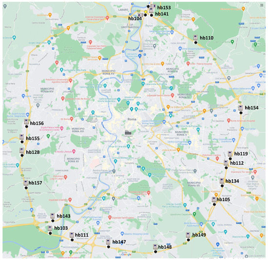
Figure 2.
Map of the acoustic sensor locations of the WASN deployed across A90 circular highway surrounding the city of Rome (suburban environment), adapted from Google Maps®.
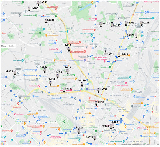
Figure 3.
Map of the acoustic sensor locations of the WASN deployed across District 9 of Milan (urban environment), adapted from Google Maps®.
Regarding the computation of STPs, on the one hand, the recorded audio signals of min length per sampled hour are parameterised by extracting energy sub-bands at the frame level using 30 ms length Hamming windows with 50% of overlap. On the other hand, the STP value of a missing point was obtained through the cubic interpolation of the values at neighboring grid points in each respective dimension, that is, in frequency and time, following [19].
As for the clustering analysis, an agglomerative hierarchical clustering technique was applied using Ward’s minimum variance algorithm [30], as it allowed both the automatic grouping of STPs and interpretation of the resulting grouping through the derived hierarchical dendrogram. The clustering analysis considered a sweep between and clusters for the suburban area, and from to clusters for the urban environment, being in both cases the total number of operative sensors per area. Four CVIs were considered to determine : (i) the ratio of within-cluster and between-cluster distances of the Davies–Bouldin index [31]; (ii) the Silhouette index [32], a measure of how similar an object is to its own cluster (cohesion) compared to other clusters (separation); (iii) the Gap value [33], which compares the within-cluster dispersion with that expected over an appropriate reference null distribution; and, (iv) the overall within-cluster variance of the Calinsky–Harabasz criterion [34].
4.1. Data Pre-Processing
For the STP computation, only those passages labelled as RTN should be considered, thus, the audio clips labelled in one of the 28 ANE identified subcategories in both environments, as well those others labelled as complex passages, where a mixture of different sound sources (e.g., diverse ANEs together with RTN as background), were removed [15].
The selection threshold has been set to , i.e., a -min audio recording was used for the corresponding STP computation if it contained at least 40% of RTN. This value was selected as a trade-off between representativeness and coverage, by ensuring the computation of mean hourly spectra of RTN considering more than 10% of the total time and assuming that less than 3% of the collected data is discarded, respectively.
Moreover, other sensed 60-min periods were also discarded due to an episode of heavy rain between 13:00 and 15:00 during the weekend in the suburban scenario. After inspection of the corresponding audio recordings, it was found that a significant number of RTN periods contained residuals of rain sound as well as their STPs presenting a significant increase in high frequency energy STPs due to the contact of tyres with wet pavement. Thus, audio data from these 1-h periods were discarded because the rain episode could have potentially biased the corresponding clustering of the STPs.
Table 1 shows the discarded 1-h periods from both suburban and urban scenarios, respectively, and provides information on the sensor name, the acoustic environment, the sensed day and the considered criterion for their identification. It can be observed that eleven periods were found in the suburban environment during the weekend day, four due to the selection threshold criteria and seven due to a rain episode. Otherwise, up to eight 1-h periods were discarded during the weekday and only one on the weekend in the urban scenario, as they did not meet the selection threshold criterion.

Table 1.
Discarded 1-h periods from both suburban and urban environments.
4.2. Analysis Results for Suburban Area
4.2.1. Interpolation of Spectro-Temporal Profiles
Figure 4 shows two examples of original and interpolated STPs for the suburban environment, both for the weekend day. First, it can be observed that the original STPs showed higher energy values at low frequency bands (below 500 Hz), due to the presence of RTN. As can be seen in the left-most graph of Figure 4a, a significant increase of the measured energy was observed at 13:00 and 15:00, which was more prominent at high frequencies. This was mainly caused by a rain episode during the weekend, which was confirmed by the ANE labels. After data interpolation, the rain effect was largely removed, as can be seen in the right-most graph of Figure 4a. Figure 4b depicts an example of a missing data period due to an insufficient number of RTN frames (below 40%) within the corresponding audio recording at 11:00. In the interpolated STP (right-most graph), the mean energy curve at this hour was filled through the cubic interpolation of the neighboring data.
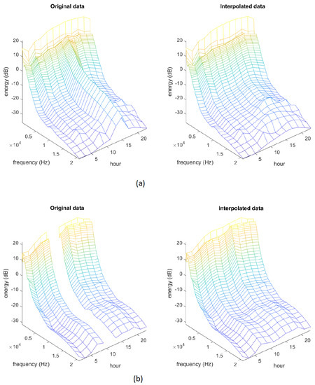
Figure 4.
Examples of original (left-side) and interpolated (right-side) STPs for the suburban environment from (a) sensor hb140 and (b) sensor hb143, respectively.
4.2.2. Weekday Suburban Analysis
Figure 5 shows the clustering validity indices curves derived from the four explored metrics using the STP data analysis from the suburban environment during the weekday. It can be observed that the solutions of (for Gap and Calinsky–Harabasz) and (for Davies–Bould and Silhouette) clusters attained local optimum values, for the Silhouette and Gap indices being the number of clusters that attained a significant increase of the validity index within the lower number of clusters.
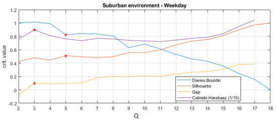
Figure 5.
Clustering validity indices obtained for the acoustic suburban environment on the weekday, resulting from the agglomerative hierarchical clustering algorithm for the considered number of clusters sweep . The suboptimal number of clusters are marked as red asterisks, being the local maxima in all clustering indices despite the Davies–Bouldin index, which is a local minimum.
Figure 6 shows the resulting dendrogram of the agglomerative hierarchical clustering for the suburban environment on the weekday, where the solutions for and are also highlighted. Figure 7 shows the obtained similarity matrix . As can be seen, the solution is compliant with the clustering solution (shown in red rectangles on the left-side), as well as (shown with white dashed lines across the image, but also as green rhomboids at the bottom of the figure). In the figure, and considering the clustering solution for , the inter (for ) and intra-cluster (for ) Euclidean distances are also shown as (note that indices i and j refer to the numeration of clusters of the solution shown in Figure 6, e.g., Ci in green).
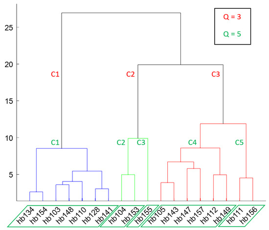
Figure 6.
Dendrogram of the agglomerative hierarchical clustering for the suburban environment on the weekday. Clustering solutions for (in red) and (in green) are also highlighted.
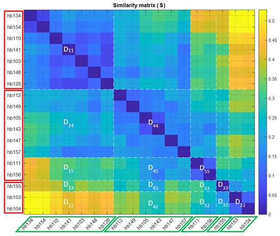
Figure 7.
Similarity matrix () for the suburban environment on the weekday. White dashed lines separate the clustering solution, which in turn also includes the optimal solution. clusters are also highlighted at the bottom by means of green rhomboids and clusters on the left-side with red rectangles. Inter () and intra-cluster () distances are highlighted in white and denoted as .
As an overall picture, Figure 7 enables us to see clearly that the clusters obtained from the STPs exhibited different patterns, with the inner similitude between sensors of each cluster being very high, because the distances in and regions were somewhat lower than the others. Due to the hierarchical nature of the clustering technique, the solution for also included the solution, where two clusters of also included two other clusters of (see Figure 6). As can also be seen from Figure 7, the sensor hb155 position has been allocated near sensors hb156 and hb111 through the expert-base analysis, because they exhibited a more similar pattern within .
4.2.3. Weekend Suburban Analysis
An equivalent clustering and analysis was conducted for the weekend, considering the corresponding STPs. First, the clustering validity indices curves are shown in Figure 8. In this case, (where Silhouette and Calinski–Harabasz indices attained local maxima) as well as (where Davies–Bouldin attained a local minimum) are the main interesting values to be considered as optimal number of clusters. The dendrogram of the agglomerative hierarchical clustering is depicted in Figure 9. Compared to the clustering solutions analysed for the weekday, it can be seen that on the weekday and during the weekend shared some similarities: (i) sensors hb111 and hb156 are grouped together; (ii) sensors hb104 and hb153 form a group on the weekday, and together with their isolate cluster with hb155 to form a new cluster at the weekend. However, the rest of the sensor locations are grouped as a whole in the solution for the weekend, while they are separated in two different clusters for the solution on the weekday.
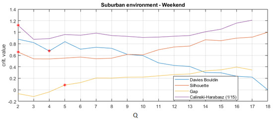
Figure 8.
Clustering validity indices obtained for the acoustic suburban environment at the weekend, resulting from the agglomerative hierarchical clustering algorithm for the considered number of clusters sweep . The suboptimal number of clusters are marked as red asterisks, being the local maxima in all clustering indices despite the Davies–Bouldin index, which is a local minimum.
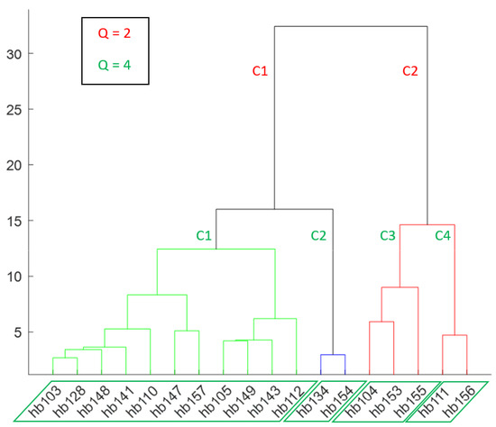
Figure 9.
Dendrogram of the agglomerative hierarchical clustering for the suburban environment at the weekend. Clustering solutions for (in red) and (in green) are also highlighted.
Figure 10 shows the similarity matrix for the suburban environment. Compared with the same matrix computed for the weekday, it can be seen that there are many similarities between both results. Looking at the differences, it is worth noting the higher distances between sensors hb134 and hb154 with respect to the most similar cluster formed by sensors hb110, hb141, hb103, hb148, and hb128 for the weekend analysis compared to its weekday counterpart (see Figure 7).
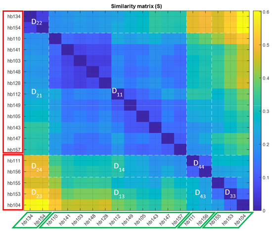
Figure 10.
Similarity matrix () for the suburban environment at the weekend. White dashed lines separate the four clusters of the clustering solution (marked as green rhomboids at the bottom), which, in turn, also includes the solution (also marked on the left-side as red rectangles). Inter- () and intra-cluster () distances are highlighted in white and denoted as .
4.3. Analysis Results for the Urban Area
4.3.1. Interpolation of Spectro-Temporal Profiles
Figure 11 shows two examples of original and interpolated STPs for the urban environment. Similar to the suburban environment, in this case, the STPs also show higher energy values at low frequency bands (below 500 Hz), due to the presence of RTN. As can be seen in the left-most graph of Figure 11a, a significant increase of the measured energy was observed at 8:00 and 14:00. In this case, it was mainly caused by an increase in various types of ANEs during these hours. After data interpolation, this increase in sound levels was smoothed, as can be observed in the right-most graph of Figure 11a. Figure 11b shows the result of interpolating a missing data period of an STP (left-most graph) due to not having enough RTN frames (below ) as a result of an episode of persistent birdsong at 14:00.
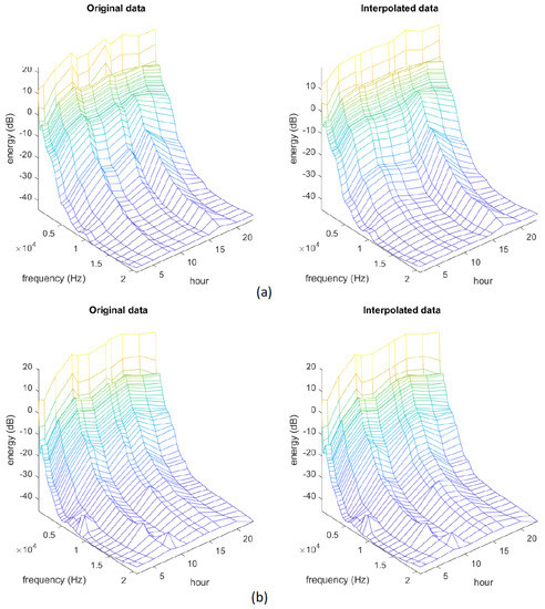
Figure 11.
Examples of original (left-side) and interpolated (right-side) STPs for the urban environment from (a) sensor hb117 and (b) sensor hb145, respectively.
4.3.2. Weekday Urban Analysis
Figure 12 shows the clustering validity indices curves derived from the four explored metrics using the STP data analysis from the urban environment on the weekday. As for the suburban analysis, the clusters solution was obtained for all the methods despite the Gap index, which attained the best suboptimum solution for clusters.
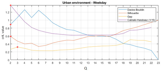
Figure 12.
Clustering validity indices obtained for the acoustic urban environment on the weekday, resulting from the agglomerative hierarchical clustering algorithm for the considered number of clusters sweep . The suboptimal number of clusters are marked as red asterisks, being the local maxima in all clustering indices despite the Davies–Bouldin index, which is a local minimum.
Figure 13 shows the dendrogram of the agglomerative hierarchical clustering for the urban environment on the weekday, where the solutions for and are highlighted in color. Moreover, Figure 14 shows the similarity matrix . As can be observed, the solution is coherent with the clustering solution (shown in red rectangles on the left-side) as well as (shown with white dashed lines across the image and also as green rhomboids at the bottom of the figure). It can be seen that, as in the suburban case, the expert-based analysis stage yields a sensor ordering where the similarity matrix presents lower Euclidean distances near its diagonal, with higher values for positions far off the diagonal, including hb133 and hb144 sensor locations with higher distances from hb109 and hb108 sensor locations. From the analysis of the similarity matrix, it can also be concluded that the sensor locations belonging to clusters C2 and C3 present more different behaviour (see higher values in region) than if they are individually compared to cluster C1 for the solution.
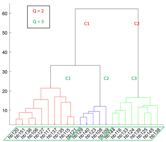
Figure 13.
Dendrogram of the agglomerative hierarchical clustering for the urban environment on the weekday. Clustering solutions for (in red) and (in green) are also highlighted.
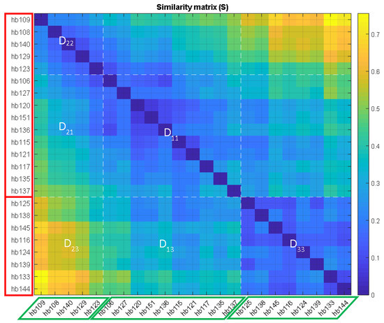
Figure 14.
Similarity matrix () for the urban environment on the weekday. White dashed lines separate three clusters of the clustering solution (marked as green rhomboids at bottom), and the one (also marked on the left-side as red rectangles). Inter () and intra-cluster () distances are highlighted in white and denoted as .
4.3.3. Weekend Urban Analysis
The same results were obtained when comparing the results of the appropriate number of clusters between the weekend and the weekday in the urban acoustic environment: was the suboptimal lower number of clusters for all the metrics, despite the Gap one, which also attained this value for clusters (see Figure 12 and Figure 15).
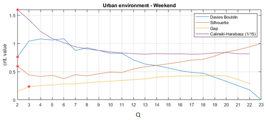
Figure 15.
Clustering validity indices obtained for the acoustic urban environment at the weekend, resulting from the agglomerative hierarchical clustering algorithm for the considered number of clusters sweep . The suboptimal number of clusters are marked as red asterisks, being the local maxima in all clustering indices despite the Davies–Bouldin index, which is a local minimum.
However, regarding the distribution of sensors within the obtained clusters with the agglomerative hierarchical clustering method, some small differences can be found when comparing weekend with weekday STPs. As can be seen in the dendrogram depicted in Figure 16, sensor locations of hb106 and hb127 were grouped together with another set of sensors, as well as hb135 and hb137. Figure 17 shows the corresponding similarity matrix of the urban weekend STPs. hb106 and hb127 seem to have behaved similarly to other sensors of cluster C1 in the solution and also other sensors from cluster C3, while the sensor location of hb135 behaved clearly closer to those from cluster C2. This pattern can also be discerned in Figure 14, but in the weekend analysis it is clearer. In contrast, the acoustic environment sensed by hb137 seems to be closer to those acoustic environments grouped in cluster C3, despite it being assigned to cluster C2.
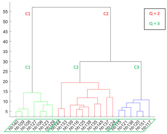
Figure 16.
Dendrogram of the agglomerative hierarchical clustering for urban environment at the weekend. Clustering solutions for (in red) and (in green) are also highlighted.
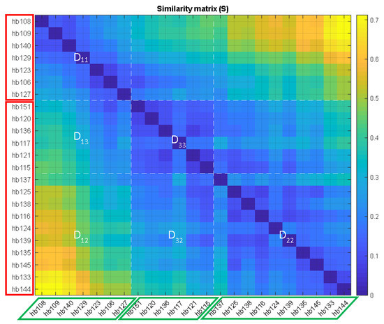
Figure 17.
Similarity matrix () for urban environment at the weekend. White dashed lines separate three clusters of the clustering solution (marked as green rhomboids at bottom), and the solution (also marked on the left-side as red rectangles). Inter () and intra-cluster () distances are highlighted in white and denoted as .
5. Discussion
Following analysis of the results, there are several aspects to be discussed. For instance, it is worth noting that the described clustering and analysis methodology has been applied to acoustic data gathered from a WASN. However, it can also be applied to other kinds of raw acoustic data obtained from N locations, e.g., from field measurement campaigns conducted by experts, if it is collected simultaneously. Nevertheless, in this example it could be more difficult to gather data 24 h/7 than using a WASN. Moreover, the clustering results obtained in both environments (urban and suburban) reinforce the need to consider acoustic data from the locations of each cluster to adapt ANED for RTN monitoring systems, and to use data from different days, as considered in this study (weekday and weekend). These results helped us to acquire a better understanding of the characteristics of RTN, with the future possibility of customizing the training and testing of the ANED algorithm in each specific location at a spectro-temporal level.
Regarding the number of clusters, they were larger in the suburban than in the urban environment. In this sense, it is worth mentioning that the sensor nodes of the Rome suburban WASN were installed on the portals along the A90 highway, considering different locations of specific road geometry, such as single roads, crossings, nearby railways and multiple connections [9,35]. This fact can probably explain why a higher number of clusters were found within this environment than were found in the urban environment where the sensors were deployed in different types of streets, but all within the same district of Milan, with less differences among locations.
The clustering analysis of the spectro-temporal patterns obtained from the RTN acoustic data can be linked to other information (e.g., related to the physical sensor location particularities) that could reinforce the STP clusters found. Regarding the suburban environment, the sensor locations can be seen in detail in [11], where it can be appreciated that all the sensors were located on the portals along the A90 highway surrounding the city of Rome in Italy, except hb104, hb153, hb155 and hb143, which were located at secondary road connections and, for the first three, at less than 500 m of the main highway crossing. From the analyses presented in Section 4.2, these three sensor locations belonged to one cluster during the weekend, while on the weekday this cluster was broken down into two groups: one composed of hb153 and hb104, and another containing only hb155. Hence, it seems that the acoustic ambient RTN presented a particular pattern, which was clearly different from the rest of the sensor locations (see large distances shown graphically in Figure 7 and Figure 10). However, sensor locations hb111 and hb156, which were also grouped together on both monitored days, seem to show a particular pattern. After inspecting their STPs, they exhibited lower energy values for the majority of hours and frequency bands, a pattern that could have been due to lower traffic density.
Considering the urban environment, the analyses conducted have shown that it is reasonable to group the sensor locations in three clusters of sensor locations on both weekdays and at weekends. In this environment, a contrast analysis can be performed considering the type of roads within the city, as previously considered in [21] to analyse the distribution of ANEs. In that study, the roads where sensors were located were divided into narrow streets (of one lane) and wide streets (with more than 1-lane). According to this classification, sensor nodes hb115, hb124, hb125, hb127, hb133, hb135, hb137, hb138, hb139, hb144 and hb145 were labelled as narrow streets, while the rest of the acoustic sensors were located in wide streets. From the clustering results presented in Section 4.3, it can be observed that clusters C1 and C2 of clustering solution on the weekday (see Figure 13) contained 100% and 87% of locations in the wide and narrow streets, respectively, while cluster C1 contained only 60% of wide streets. In addition, during the weekend (see Figure 16), clusters C1 and C3 of clustering contained 85% and 83% of wide streets, while cluster C2 contained up to 90% of narrow street locations. As the type of street affects the acoustic environment (e.g., the canyon effect in narrow streets [36]), this reinforces the results obtained.
6. Conclusions
In this study, an analysis and clustering methodology has been proposed to group RTN acoustic data by considering the spectro-temporal energy distribution of a set of recordings gathered simultaneously from an area of interest during a given period of time. The proposal has been evaluated in two different environments, either urban and suburban, using approximately 250 h of RTN data collected through operative WASNs of the DYNAMAP project over two different days (a weekday and weekend day). The obtained set of clusters have been analysed by experts, obtaining a similarity matrix that shows graphically the Euclidean distances between specific RTN STPs from the sensed locations.
From the analyses conducted, it can be concluded that the weekday and weekend patterns shared many similarities, and even when certain locations were grouped differently, on both days (e.g., in the urban environment, up to three clusters were obtained on both days, differing only in 4 out of 23 sensor locations), which supports the idea of considering weekday and weekend to have different RTN behaviour at a spectro-temporal level. These findings could be considered to support decision-making by administrations or private entities supervising roads and traffic, to evaluate the effects of action plans in real time, and develop new policies to improve the quality of life of their citizens. It is of note that the clustering analysis in the suburban environment revealed more heterogeneity, i.e., a higher number of clusters was obtained (with up to five clusters in the weekday analysis), than in the urban environment (where partitions were quite highly correlated with the type of streets in terms of number of lanes). The higher homogeneity found in the urban environment could be harnessed to the detection of possible variations or anomalies in real-time through monitoring systems, including those provoking sudden changes in spectro-temporal patterns, e.g., those derived from the COVID-19 pandemic.
Future research will be developed to consider the viability of the proposed clustering and analysis methodology from the results found in this study. To do so, data derived from other sources of information (e.g., traffic monitoring systems) could also be considered to deepen the analyses performed to better understand the main reasons for the similarities and differences found between the set of clustered locations. This more precise knowledge will enable us to obtain, on the one hand, better RTN models that can be used for the development of more accurate ANED algorithms that can be trained specifically for each clustered RTN environment and, on the other hand, to enrich RTN monitoring systems with valuable information that could be used to support the development of specific actions for real-time traffic management in urban and suburban environments.
Author Contributions
Conceptualization, F.A.; methodology, J.C.S., F.A. and R.M.A.-P.; software, J.C.S.; validation, F.A.; data curation, J.C.S.; writing—original draft preparation, F.A. and J.C.S.; writing—review and editing, F.A., J.C.S. and R.M.A.-P.; visualization, J.C.S.; supervision, F.A. All authors have read and agreed to the published version of the manuscript.
Funding
This research received no external funding.
Conflicts of Interest
The authors declare no conflict of interest.
Abbreviations
The following abbreviations are used in this manuscript:
| ANE | Anomalous noise event |
| ANED | Anomalous noise event detector |
| CNOSSOS-EU | Common Noise Assessment Methods in Europe |
| DYNAMAP | Dynamic noise mapping |
| END | European Noise Directive |
| IR | Intermittency ratio |
| RTN | Road traffic noise |
| SNR | Signal-to-noise ratio |
| SPL | Sound pressure level |
| STP | Spectro-temporal profile |
| WASN | Wireless acoustic sensor network |
References
- Babisch, W.; Beule, B.; Schust, M.; Kersten, N.; Ising, H. Traffic noise and risk of myocardial infarction. Epidemiology 2005, 16, 33–40. [Google Scholar] [CrossRef] [PubMed]
- Muzet, A. Environmental noise, sleep and health. Sleep Med. Rev. 2007, 11, 135–142. [Google Scholar] [CrossRef] [PubMed]
- Alberts, W.; Roebben, M. Road Traffic Noise Exposure in Europe in 2012 based on END data. In Proceedings of the 45th International Congress and Exposition on Noise Control Engineering (INTER-NOISE 2016), Hamburg, Germany, 21–24 August 2016; pp. 1236–1247. [Google Scholar]
- EU. Directive 2002/49/EC of the European Parliament and the Council of 25 June 2002 relating to the assessment and management of environmental noise. Off. J. Eur. Communities 2002, L189/12. [Google Scholar]
- The European Commission. Commission Directive (EU) 2015/996 of 19 May 2015. Available online: https://eur-lex.europa.eu/legal-content/EN/TXT/PDF/?uri=CELEX:32015L0996&from=PT (accessed on 30 December 2021).
- Alías, F.; Alsina-Pagès, R.M. Review of Wireless Acoustic Sensor Networks for Environmental Noise Monitoring in Smart Cities. J. Sens. 2019, 2019, 13. [Google Scholar] [CrossRef] [Green Version]
- Sevillano, X.; Socoró, J.C.; Alías, F.; Bellucci, P.; Peruzzi, L.; Radaelli, S.; Coppi, P.; Nencini, L.; Cerniglia, A.; Bisceglie, A.; et al. DYNAMAP—Development of low cost sensors networks for real time noise mapping. Noise Mapp. 2016, 3, 172–189. [Google Scholar] [CrossRef]
- Zambon, G.; Benocci, R.; Bisceglie, A. Development of optimized algorithms for the classification of networks of road stretches into homogeneous clusters in urban areas. In Proceedings of the 22nd International Congress on Sound and Vibration (ICSV22), Florence, Italy, 12–16 July 2015; pp. 1–8. [Google Scholar]
- Bellucci, P.; Peruzzi, L.; Zambon, G. Life Dynamap project: The case study of Rome. Appl. Acoust. 2017, 117, 193–206. [Google Scholar] [CrossRef]
- Alías, F.; Socoró, J.C.; Orga, F.; Alsina-Pagès, R.M. Characterization of a WASN-based Urban Acoustic Dataset for the Dynamic Mapping of Road Traffic Noise. In Proceedings of the 6th International Electronic Conference on Sensors and Applications (ECSA-6), On-Line, 15–30 November 2019. [Google Scholar] [CrossRef] [Green Version]
- Alsina-Pagès, R.M.; Orga, F.; Alías, F.; Socoró, J.C. A WASN-Based Suburban Dataset for Anomalous Noise Event Detection on Dynamic Road-Traffic Noise Mapping. Sensors 2019, 19, 2480. [Google Scholar] [CrossRef] [PubMed] [Green Version]
- Mermelstein, P. Distance measures for speech recognition, psychological and instrumental. Pattern Recognit. Artif. Intell. 1976, 116, 374–388. [Google Scholar]
- Socoró, J.C.; Alías, F.; Alsina-Pagès, R.M. An Anomalous Noise Events Detector for Dynamic Road Traffic Noise Mapping in Real-Life Urban and Suburban Environments. Sensors 2017, 17, 2323. [Google Scholar] [CrossRef] [PubMed]
- Alías, F.; Alsina-Pagès, R.M.; Orga, F.; Socoró, J.C. Detection of Anomalous Noise Events for Real-Time Road-Traffic Noise Mapping: The DYNAMAP’s project case study. Noise Mapp. 2018, 5, 71–85. [Google Scholar] [CrossRef]
- Alías, F.; Orga, F.; Alsina-Pagès, R.M.; Socoró, J.C. Aggregate Impact of Anomalous Noise Events on the WASN-Based Computation of Road Traffic Noise Levels in Urban and Suburban Environments. Sensors 2020, 20, 609. [Google Scholar] [CrossRef] [Green Version]
- Brambilla, G.; Benocci, R.; Confalonieri, C.; Roman, H.E.; Zambon, G. Classification of urban road traffic noise based on sound energy and eventfulness indicators. Appl. Sci. 2020, 10, 2451. [Google Scholar] [CrossRef] [Green Version]
- Pita, A.; Rodriguez, F.J.; Navarro, J.M. Cluster Analysis of Urban Acoustic Environments on Barcelona Sensor Network Data. Int. J. Environ. Res. Public Health 2021, 18, 8271. [Google Scholar] [CrossRef] [PubMed]
- Xue, W.; Huang, Z.; Zhao, B.; Yang, W.; Lan, Z.; Cai, M. Updated traffic noise map method based on speed cluster. Appl. Acoust. 2021, 175, 107818. [Google Scholar] [CrossRef]
- Socoró, J.C.; Alsina-Pagès, R.M.; Alías, F.; Orga, F. Acoustic Categorization of the urban Multi-Sensor Network of the DYNAMAP LIFE project developed for Road Traffic Noise Mapping. In Proceedings of the Inter-Noise 2019, Madrid, Spain, 16–19 June 2019; pp. 1–12. [Google Scholar]
- Socoró, J.C.; Alías, F.; Alsina-Pagès, R.M. Spectro-temporal analysis of road traffic noise in the rome and milan pilot areas of the DYNAMAP project. In Proceedings of the 27th International Congress on Sound and Vibration (ICSV 2021), On-Line, 11–16 July 2021; pp. 1–8. [Google Scholar]
- Alías, F.; Socoró, J.C.; Alsina-Pagès, R.M. WASN-Based Day–Night Characterization of Urban Anomalous Noise Events in Narrow and Wide Streets. Sensors 2020, 20, 4760. [Google Scholar] [CrossRef] [PubMed]
- Camps-Farrés, J.; Casado-Novas, J. Issues and challenges to improve the Barcelona Noise Monitoring Network. In Proceedings of the EuroNoise 2018, Crete, Greece, 27–31 May 2018; pp. 693–698. [Google Scholar]
- Lan, Z.; He, C.; Cai, M. Urban road traffic noise spatiotemporal distribution mapping using multisource data. Transp. Res. Part D Transp. Environ. 2020, 82, 102323. [Google Scholar] [CrossRef]
- Zambon, G.; Bisceglie, A. Milan dynamic noise mapping from few monitoring stations: Statistical analysis on road network. In Proceedings of the 45th International Congress and Exposition on Noise Control Engineering (InterNoise 2016), Hamburg, Germany, 21–24 August 2016; pp. 6531–6542. [Google Scholar]
- Zambon, G.; Benocci, R.; Brambilla, G. Cluster categorization of urban roads to optimise their noise monitoring. Environ. Monit. Assess. 2016, 188, 26. [Google Scholar] [CrossRef] [PubMed] [Green Version]
- Zambon, G.; Benocci, R.; Bisceglie, A.; Roman, H.E.; Bellucci, P. The LIFE DYNAMAP project: Towards a procedure for dynamic noise mapping in urban areas. Appl. Acoust. 2017, 124, 52–60. [Google Scholar] [CrossRef]
- Wunderli, J.M.; Pieren, R.; Habermacher, M.; Vienneau, D.; Cajochen, C.; Probst-Hensch, N.; Röösli, M.; Brink, M. Intermittency ratio: A metric reflecting short-term temporal variations of transportation noise exposure. J. Expo. Sci. Environ. Epidemiol. 2016, 26, 575–585. [Google Scholar] [CrossRef] [PubMed]
- Benocci, R.; Confalonieri, C.; Roman, H.E.; Angelini, F.; Zambon, G. Accuracy of the dynamic acoustic map in a large city generated by fixed monitoring units. Sensors 2020, 20, 412. [Google Scholar] [CrossRef] [PubMed] [Green Version]
- Valero, X.; Alías, F. Gammatone Cepstral Coefficients: Biologically Inspired Features for Non-Speech Audio Classification. IEEE Trans. Multimed. 2012, 14, 1684–1689. [Google Scholar] [CrossRef]
- Ward, J.H., Jr. Hierarchical Grouping to Optimize an Objective Function. J. Am. Stat. Assoc. 1963, 58, 236–244. [Google Scholar] [CrossRef]
- Davies, D.; Bouldin, D.W. A Cluster Separation Measure. IEEE Trans. Pattern Anal. Mach. Intell. 1999, 1, 224–227. [Google Scholar] [CrossRef]
- Rousseeuw, P.J. Silhouettes: A graphical aid to the interpretation and validation of cluster analysis. J. Comput. Appl. Math. 1987, 20, 53–65. [Google Scholar] [CrossRef] [Green Version]
- Tibshirani, R.; Walther, G.; Hastie, T. Estimating the number of clusters in a data set via the gap statistic. J. R. Stat. Soc. Ser. B 2001, 63, 411–423. [Google Scholar] [CrossRef]
- Caliński, T.; Harabasz, J. A dendrite method for cluster analysis. Commun. Stat. 1974, 3, 1–27. [Google Scholar] [CrossRef]
- Benocci, R.; Bellucci, P.; Peruzzi, L.; Bisceglie, A.; Angelini, F.; Confalonieri, C.; Zambon, G. Dynamic Noise Mapping in the Suburban Area of Rome (Italy). Environments 2019, 6, 79. [Google Scholar] [CrossRef] [Green Version]
- Echevarria-Sanchez, G.M.; Van Renterghem, T.; Thomas, P.; Botteldooren, D. The effect of street canyon design on traffic noise exposure along roads. Build. Environ. 2016, 97, 96–110. [Google Scholar] [CrossRef] [Green Version]
Publisher’s Note: MDPI stays neutral with regard to jurisdictional claims in published maps and institutional affiliations. |
© 2022 by the authors. Licensee MDPI, Basel, Switzerland. This article is an open access article distributed under the terms and conditions of the Creative Commons Attribution (CC BY) license (https://creativecommons.org/licenses/by/4.0/).