Abstract
A series of Generative Adversarial Networks (GANs) could effectively capture the salient features in the dataset in an adversarial way, thereby generating target data. The discriminator of GANs provides significant information to update parameters in the generator and itself. However, the discriminator usually becomes converged before the generator has been well trained. Due to this problem, GANs frequently fail to converge and are led to mode collapse. This situation can cause inadequate learning. In this paper, we apply restart learning in the discriminator of the GAN model, which could bring more meaningful updates for the training process. Based on CIFAR-10 and Align Celeba, the experiment results show that the proposed method could improve the performance of a DCGAN with a low FID score over a stable learning rate scheme. Compared with two other stable GANs—SNGAN and WGAN-GP—the DCGAN with a restart schedule had a satisfying performance. Compared with the Two Time-Scale Update Rule, the restart learning rate is more conducive to the training of DCGAN. The empirical analysis indicates four main parameters have varying degrees of influence on the proposed method and present an appropriate parameter setting.
1. Introduction
Ever since the advent of Generative Adversarial Networks [1], many studies have focused on ways to improve the quality and diversity of the generated images. Deep-Convolutional Generative Adversarial Networks (DCGAN) [2] are one of the examples which has shown significant improvements in the history of GANs research. DCGAN combines a GAN and convolutional network and imposes a series of constraints on the architecture to make it more stable. Since then, DCGAN-based architectures have been applied to different kinds of other GAN architectures. For example, Wasserstein distance was proposed as a standard measurement in [3]. Karras et al. [4] has proposed Progressive Growing of GANs (ProGAN) which is a progressive network training method that significantly improves the speed, stability, and quality of image generation. Large Scale GAN (BigGAN) [5] focuses on training networks in large scale, and improves the orthogonal regularization of generators to produce images with high fidelity and diversity. Self-Attention GAN (SAGAN) [6] generates details on a given image by allowing attention-driven, long-range dependency modeling for image generation tasks. A style-based Generator Architecture for GAN (StyleGAN) [7] improves the ability of GANs by fine-controlling the generated images, and thereby makes outstanding contributions to GAN synthesis. Sliced Wasserstein Generative Adversarial Networks (Sliced WGAN) [8] maps high-dimensional distribution to one-dimensional marginal distribution, which solves the problem of calculating Wasserstein distance in high-level space. The works mentioned above have extended the GANs’ architecture in order to achieve improved performance. However, the problem in terms of the instability and difficulty of training the GAN model remains not completely resolved [9,10,11,12]. In recent years, some researchers have focused on the study of the training process. It is well known that the judgment results of the discriminator provide an indication for updating generator parameters in GAN. Additionally, as aforementioned, the discriminator can be converged before the generator is well trained during the training phase. Therefore, the converged discriminator returns no gradient to the generator for updating its parameters. Arjovsky and Bottou [13] have discussed the phenomenon and argued that this problem is because the distribution of the generator is not continuous or the supports of generator and discriminator are disjoint. A solution in [13] is adding continuous noises to the inputs of the discriminator, therefore smoothing the distribution of the probability mass to ensure the discriminator is generated. Another one in [14] is an adaptive learning scheme for learning rate, which is carried out by comparing the KID score (proposed in [14]) from the previous iteration with KID score derived currently. The above two methodologies stabilize the GANs’ training process efficiently while they are also accompanied by extra heavy computing cost. The authors in [15] found a reasonable annealing scheme is a benefit for training GANs by avoiding model collapse. Different from the simple application in the above paper, our annealing scheme follows a cosine annealing function in each restart period and the peak values follow another annealing scheme in the whole process. The authors of [16] proved that the GANs models could converge to a local Nash equilibrium with different learning rates for training discriminator and generator, which reminds us of the feasibility to study the learning rate of the two networks separately.
In this paper, we use a restart learning rate [17] instead of a stable learning rate in the discriminator. Our insight is that the restart learning method could dig deeper into the attributes of target data and bring more benefits from periodical changes on the learning rate to prevent from a fast convergence of the discriminator. Thus, we train the discriminator in GAN by implementing a restart learning algorithm.
Our formula of restart learning rate is motivated by these papers: instead of monotonically annealing the learning rate, Smith [17] lets the learning rate cyclically vary between reasonable boundary values to improve classification accuracy; Loshchilov et al. [18] focus on the restart to make it more flexible and gives alternative schedule schemes (with different initial cycle lengths and its increased control coefficient in each cycle). In addition to extending the cycle length in the next cycle, we also performed experiments on shortened cycle length and different initial cycle length values with settings as in [18]. Moreover, with the above schedule in [18], we also control peak value by coefficient and set the baseline of amplitudes ; Huang et al. [19] updated the learning rate at each iteration rather than at every epoch, which improves the convergence of short cycles even when a large initial learning rate is used. Compared with the cyclic cosine learning rate of the Snapshot Ensemble algorithm in [19], we set the baseline to rate avoiding property of its disappearing and performed experiments with various peak values by coefficient instead of only one value 0.5. In recent years, the restart idea is applied to several research areas: Xingjian Li [20] followed cyclical learning rates mentioned in [17] to do deep transfer learning; Wang et al. [16] restarted the momentum in algorithm to reduce error accumulation in stochastic gradient.
Against these backgrounds, we try to do a deeper and more detailed study on the restart learning scheme in GAN, and our main contributions are as follows:
- We discussed the adaptability of the restart learning mechanism applied to training the discriminator. To our knowledge, our research is the first attempt to apply the restart learning scheme in GAN training and which is different from adaptive learning and the simple annealing scheme in other GAN papers.
- With our methodology, we could avoid the problem of vanishing the generator’s gradient and obtain improved performance in the experiment results.
- We applied two annealing mechanisms in the training process: the annealing in the whole process and the annealing in each cycle. The first one is same as the method as in [15].
- For four main parameters in our design: cycle length control coefficient , peak value control coefficient , the baseline of amplitudes , and the number of steps in the first cycle P, we perform thorough ablation study to explore their influences and find appropriate values for them.
Overall, we apply the restart learning rate to the training process of the discriminator instead of a stable value. Our proposed method has improved the performance of GANs, as indicated by our experiment results.
2. Statement of Problem
2.1. GANs
In 2014, Ian J. Goodfellow proposed an adversarial framework called GAN to estimate generative models [1]. Since then, a series of GANs has been proposed gradually, like DCGAN [2], WGAN [3], BigGANs [5], etc. In GANs, there are two networks, generator (G) and discriminator (D). G trys to learn the distribution of target data x with input prior , where z is random noise. In the meanwhile, D tries to distinguish between generated data and target data. If this min-max game reaches equilibrium, G can output data with the similar distribution of target data x, and therefore, the classification accuracy of D will be close to . This means that D is unable to effectively differentiate between the generated data and the target data [1].
In the above function, is the target value function of GAN which is given by D and G, where x is target data, z is random noise, is the probability distribution of target data x, is the probability distribution from the generator with noise z as input, is the discriminator’s decision whether its input comes from the target data, and is the discriminator’s decision whether its input is generated from the generator.
At the beginning of the training phase, D attempts to estimate target data x as 1 and generated data as 0. By updating the parameters of D, we use a loss function as defined in Equation (2) to perform the back-propagation procedure. The equation basically calculates the loss of target data x (i.e., ) and the generated data (i.e., ). However, we train G with a loss function as shown in Equation (3) which computes the loss of D when it estimates generated data .
Based on Equation (2), as aforementioned, we expect a high value from and a low value from so that the D can distinguish the generated data as false data and target data as true data effectively. In other words, in terms of log values, the higher the value from and , the better the performance of D is. Therefore, we optimize D by maximizing the Equation (2).
On the other hand, in order to optimize G, we expect D predicts as true with a high probability. Hence, we update the parameters of G by minimizing Equation (3).
2.2. Problem of GANs
From Equations (2) and (3), we can observe that the loss value of D has an important role to update both D and G. In an ideal situation, G receives a sufficient amount of gradients for updating its parameters in order to generate a new datum that is similar to a datum in target data at the beginning of the training phase; on the other hand, D receives a small amount gradients to prevent it to be converged before G has been well trained. In summary, we expect G can be converged first so that D has difficulty in distinguishing between target data and generated data. Unfortunately, the reality shows that D is always converged first in the experiments as shown in the blue line in Figure 1a while loss of G in Figure 1b (blue line) increases rapidly because G lacks sufficient gradients.
Figure 1.
Loss lines with a constant learning rate (blue line) and restart learning rate (red line). (a) shows the losses in D where it is a composition of and , (b) refers to the losses in G, (c) illustrates the losses when D has predicted a target image as a generated image (), and (d) depicts the losses when D distinguishes a generated image as a target image ().
Figure 1 shows four graphs associated with different loss values either applying a constant learning rate (blue line) or restart learning rate (red line) in DCGAN. Figure 1a shows the losses in D where each of them is a composition of and , Figure 1b refers to the losses in G, Figure 1c illustrates the losses when D mistakes a target image as a generated image (), and Figure 1d depicts the loss when D mistakes a generated image as a target image (). The blue line represents a loss when a fixed learning rate (i.e., we set it as 0.001 during the experiments) is used, and the red line refers to the loss with the restart learning rate (i.e., the initial value is set as 0.001 for all experiments) during the training phase.
Figure 1 shows the D loss as a main provider for optimizing D and G. However, the longer we train, the smaller the loss we have for D which can be observed in Figure 1a. From Figure 1a, we notice the lowest loss value that we have is lower than 0.2 at the later stage. This phenomenon directly influences the loss of G which increases rapidly during the training as depicted in Figure 1b. This means that D has converged and G’s gradients have vanished. From Figure 1c,d, we observe that converges faster than . This shows that the vanishing of is mainly due to the convergence of . In other words, D distinguishes most generated images as fake, and G cannot learn properly from the loss of D. In the future, we will do more study on the reason why converges too fast.
As aforementioned, G should be able to generate a fake image that has the same probability to be predicted as a true image or a fake image by D. That is, is expected to be close to 0.5. In contrast, the model is not well trained because the vanishing gradient has occurred during the training of G. Although the use of restart learning rate brings fluctuations to the loss, it prevents the blind reduction of effectively as shown in the red line of Figure 1a and improves the performance of G by producing lower loss values than the use of stable learning rate, as shown in the red line of Figure 1b.
3. DCGAN with Restart Learning Rate
As a representative model in GANs, DCGAN significantly improves the architectural topology of a GAN to make it stable to be trained in most settings. In this paper, DCGAN is chosen to be the basic model for studying the influence of restart learning rate in D of GANs.
3.1. Cosine Decay Learning Rate
During the training phase, the learning rate usually controls the updating speed of parameters. When the learning rate is small, the updating speed will be greatly reduced. In contrast, oscillations will occur in the process, causing the parameters to linger near the optimal value. We introduce the restart learning into the training discriminator. In each restart period, we follow a cosine annealing schedule [19]. Unlike the traditional learning rate, the restart learning rate drops gradually at first, and then later rises sharply again as the number of epochs increases as shown in Figure 2.
Figure 2.
Restart Learning Rate: (a) learning rate with different restart cycles; (b) learning rate with different restart peaks; (c) Learning rate with different minimum learning rate decays.
The reason for taking the above measure is to prevent the model to be stuck in and to search only in the local minimum. In other words, with the above measure, we want to move out from the local minimum quickly which also overcomes the saddle problem [21]. Noted that the saddle problem refers to the first iteration, the learning rate of cosine annealing drops rapidly which allows the model to step into the local optimum regardless the local minimum is either steep or not; in the next iteration, due to the large value increment on the learning rate, the model can escape from the current local optimum and search new and more optimal points. The descent of cosine function simulates the process of finding potential regions with a large learning rate, and then quickly converging with a small learning rate. The best minimum point indicates that G can generate high-quality images. Our assumption is that if D has been trained with different local minimum points, then it will effectively mitigate the model collapse problem.
The function is explained as follows:
where is the count of current steps, indicates the number of steps that will be delayed in a cycle (Figure 2a), and is a cosine function. In order to prevent the value of the decay line lower than a certain value, we introduce into Equation (5). Figure 2c shows the value of learning rate with different values.
The learning rate in D will be updated as follows:
3.2. Restart Learning Rate in Discriminator
In GANs, if the convergence speed of the discriminator is too fast, then it can lead to the failure of model training. If the loss value of the discriminator is closer to 0, then the loss value neither guides the generator to find the local minimum nor explore more areas. This affects both the quality and the diversity of the generated results. Therefore, we introduce the restart learning rate which can be reset periodically during the learning process. This method does not only prevent the loss value of the discriminator to be closer to 0, but it also provides an effective gradient for G during the back-propagation procedure. Besides that, the sudden increase in the learning rate at the beginning of each cycle is conducive to the model to explore more areas and increases the diversity of results. Overall, applying the restart learning algorithm in the discriminator can overcome the generator’s problem and improve the quality and diversity of the results. In the practical experiments, we must admit that a sudden increase in the restart learning rate in the next cycle will cause significant interference to the training process. In the early stage of training, the advantages of this interference outweigh the disadvantages, similar to algorithms that add noise to the training samples. However, during the training process, the model gradually finds an area near the optimal point in a flat place, and then this interference will cause shocks, which gives more disadvantages than benefits. Therefore, we use the parameter to gradually reduce the peak learning rate of each cycle to relieve the shock at the end of training.
where i is the index of number of period, and is a parameter used to increase (i.e., 2) or decrease (i.e., 0.5) the cycle length. Noted that in Equation (7) returns only integer value.
We provide the pseudo-code of our proposed method in Algorithm 1. The inputs include the number of updates in the first cycle denoted as P, and the number of all updates denoted as t. We initialize hyper-parameters used in the restart learning rate method, such as the original learning rate , an amplitude control parameter , and the baseline of amplitude . Parameter in the DCGAN network is initialized as 0. We use ADAM optimizer [22] during the back-propagation procedure. Noted that the restart learning rate can be applied to any optimizer. In ADAM, is ‘bias-corrected first moment estimate’ and is ‘bias-corrected second raw moment estimate’.
For each step, the discriminator is updated by the ADAM optimizer. In the meanwhile, the restart learning rate, introduced at line 5, will be updated at every step. The steps of the first cycle are determined by the initial P. After that, the length of the current cycle will be determined by parameter (at line 6). Note that the cyclical restart learning rate does not restart completely (i.e., not from zero) in each cycle, but its update is based on the last learning rate from the previous cycle.
| Algorithm 1 Restart Learning Rate in discriminator of DCGAN |
| Input: first decay steps P, steps t |
| Output: |
| 1: Initialize learning rates , ,, weights |
| 2: The procedure of updating : |
| 3: for steps do |
| 4: |
| 5: |
| 6: |
| 7: Backpropagation with ADAM Optimizer |
| 8: |
| 9: End for |
4. Evaluation
4.1. Settings
We want to demonstrate that our method could improve performance by enhancing the stability of GAN training. However, there are different GAN architecture designs and parameters settings in GAN papers. For fairness, we have done all experiments with the same architecture and shared parameters of their proposed approaches in different GANs. We set DCGAN model settings in [2] to be the baseline, and we trained different GAN architectures based on DCGAN while holding their own method: for SNGAN, we used spectral normalization instead of batch normalization [9]; for WGAN-GP, we removed sigmoid function in the layer which no longer took log loss [3] and penalized the norm of the gradient of the critic with respect to its input [23].
All experiment programs run on a computer with the following configuration: Intel Core i9-9900k CPU, 3.6 GHz, x64 processor, 2080Ti GPU.
4.2. Data
We have implemented our experiments on CIFAR-10 and Align Celeba. CIFAR-10 contains 60,000 images with 10 different classes and the image size is 32 * 32. Align Celeba contains 202,599 face aligned and cropped images, and we clip each image size to 64 * 64. As we performed experiments for unsupervised learning, we only trained GANs on images regardless of their labels.
4.3. Evaluation Standard
As we know, the Inception Score (IS) and Frechet Inception Distance (FID) can measure the quality and variety of generated images as two popular metrics in measuring the performance of GAN. According to [24], FID captures the similarity of generated images to real ones better than Inception Score, especially for the robustness to noise and mode collapse (G produces a limited variety of samples). So we use FID as a metric to evaluate the learning ability of the GAN model with different learning schemes including our proposal. FID is calculated as follows:
Note that is the distribution of real images and is the distribution of generated images. FID is a metric used for measuring the distance between the feature vector of the real images and that of the generated images. The lower the score, the more similar the two groups of images are, or the more similar their statistics are. The best-case FID score is 0.0, which means that the two groups of images are the same.
4.4. Result Analysis
Firstly, we ran our method on different data sets (CIFAR-10, single class images in CIFAR-10 and Align CelebA) to check its efficiency in generation results. Table 1 shows that we have obtained different results (measured with FID) when we performed the experiments with stable and restart ( means the learning rate in discriminator). In the experiments, we used the same DCGAN structure but different inputs. In the first row, the input is the whole CIFAR-10, and the input in the last row is Align Celeba. We also checked the availability of our method in single class images in CIFAR-10 and present them in other rows. From the results in 
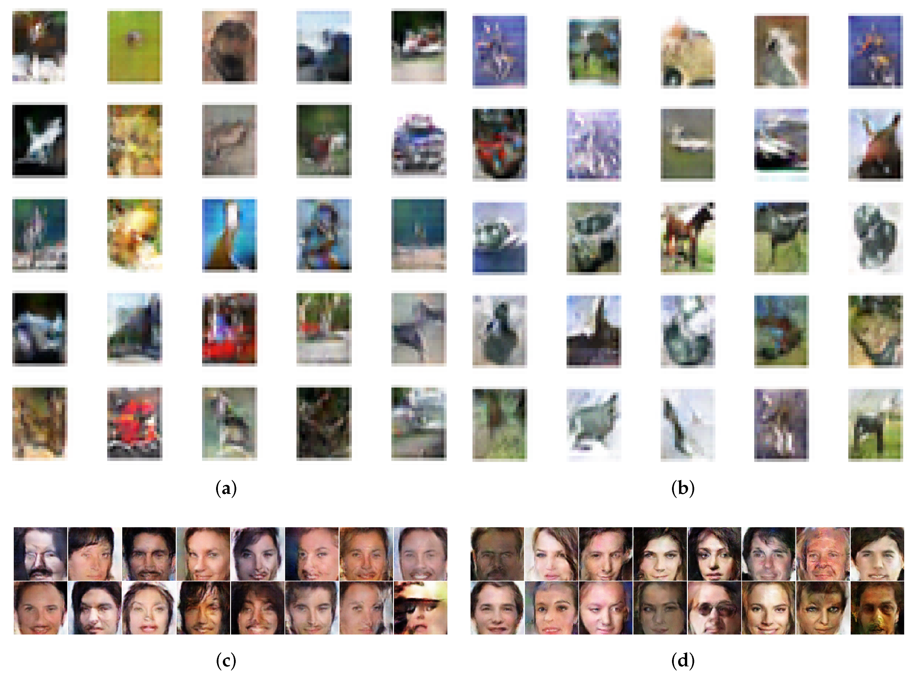
Table 1, we could see that the performance of the DCGAN trained with restart learning rate has shown different degrees of improvement on multi-category data (shown in the first row and the last row) and single-category data in CIFAR-10 (shown in the other rows). We also presented the corresponding visual results in Figure 3: when we trained DCGAN with stable on CIFAR-10, there are blurred parts in (a), while (b) has exhibited higher image resolution; on Align Celeba, almost all the faces in (c) are distorted and the use of Restart could decrease the faces distortion (shown in (d) of Figure 3). In conclusion, the plunge of Restart is beneficial to GAN in terms of generation ability. In the next experiments, we will see whether these improvements come from the improvement of networks stability.
Table 1.
Performance of DCGAN trained with stable learning rate and restart learning rate in 10,000 iterations for different datasets: (1) CIFAR-10; (2) single class in CIFAR-10 (3); Align Celeba.
Figure 3.
Visual results trained with Restart of DCGAN on CIFAR-10 and Align Celeba. (a) DCGAN trained with Stable on CIFAR-10. (b) DCGAN trained with Restart on CIFAR-10. (c) DCGAN trained with Stable on Align Celeba. (d) DCGAN trained with Restart on Align Celeba.
Table 2 shows the generated results (measured by FID score) by various GANs on CIFAR-10. We performed these experiments in different GANs for two purposes: (1) SNGAN and WGAN-GP are typical GANs to stable the training process, so we want to compare our method with SNGAN and WGAN-GP; (2) as our method only affects learning rate, we also want to check if it can improve the performance in SNGAN and WGAN-GP.
Table 2.
Generated FID results on CIFAR-10 with stable/restart learning rate in different GANs: DCGAN [2]; SNGAN [9]; WGAN-GP [23]. Bold denotes the smallest distance.
Note that when we performed the experiments in Table 1, we tried to train models sufficiently (total updates = 100 k) with apposite learning rate value. However in the experiments of Table 2, what we want to prove is that our restart schedule could improve the performance in various GANs despite of different initial learning rates and training steps. So we have different parameter settings for experiments in Table 1 and experiments in the DCGAN model of Table 2.
The learning rate for GANs training is usually around (or ), and a large learning rate always causes oscillation over training steps. In Table 2, when we set stable to be (or ), the more steps we take, the worse results we obtain in DCGAN and SNGAN (i.e., column 1 of Table 2), which indicates the oscillation. Application of the restart learning rate in discriminator will avoid the oscillation problem effectively and brings more meaning for gradients for training, even though the maximum of Restart is also set to be (i.e., the column 2 of Table 2).
When we set learning rate to be a relatively small value , the restart learning rate could still promote the performance of DCGAN and SNGAN (shown in column 3 and column 4 of Table 2). In practice, is usually our choice for training process. Thus, under this value, we run experiments of each GAN five times to calculate its average and standard deviation of FID to check the impact of our proposed method on stability.
When we use stable , WGAN-GP performed well in both cases (i.e., and ) which means WGAN-GP stabilizes training process efficiently while the use of restart in it lead to worse results (i.e., line 5 and line 6 of Table 2). We think there are two reasons: (1) WGAN-GP has already stable the training, hence periodical restart learning rate brings interference (can be indicated by the standard deviation of FID). (2) The reason why the restart learning rate is effective in DCGAN and SNGAN is that it avoids the disappearance of , while the loss in the discriminator of WGAN-GP depends on Earth Mover (EM) distance which is continuous and differentiable till optimality. Bold numbers in Table 2 means the best results in three GANs respectively. WGAN-GP with stable (FID = 59.245) and DCGAN with restart (FID = 58.735) have obtained the highest comparable performance in 40k iterations. Table 2 shows that restart is beneficial to DCGAN and SNGAN (with low average FID and comparable standard deviation value) but is not available for WGAN-GP. Exploring the deep reason why restart learning rate is useful or useless in various GAN frameworks is one of our future research directions.
Table 3 records the time spent for DCGAN and WGAN-GP to reach the best results (shown in bold) in Table 2. As we have mentioned in the above paragraph, DCGAN with this restart and WGAN-GP with stable have comparable results in 40k iterations while DCGAN with this restart spent less time. The reason why WGAN-GP with stable cost more time is that it needs to calculate penalty in every iteration. We also note that the restart schedule does not bring too many calculations (compare line 1 and line 2 of Table 3). All in all, the restart learning rate improves the generation performance of DCGAN without too much computational complexity and it is meaningful for GANs training. DCGAN with restart is a reasonable choice for GANs generation work.
Table 3.
Time spent in 40k iterations on CIFAR-10.
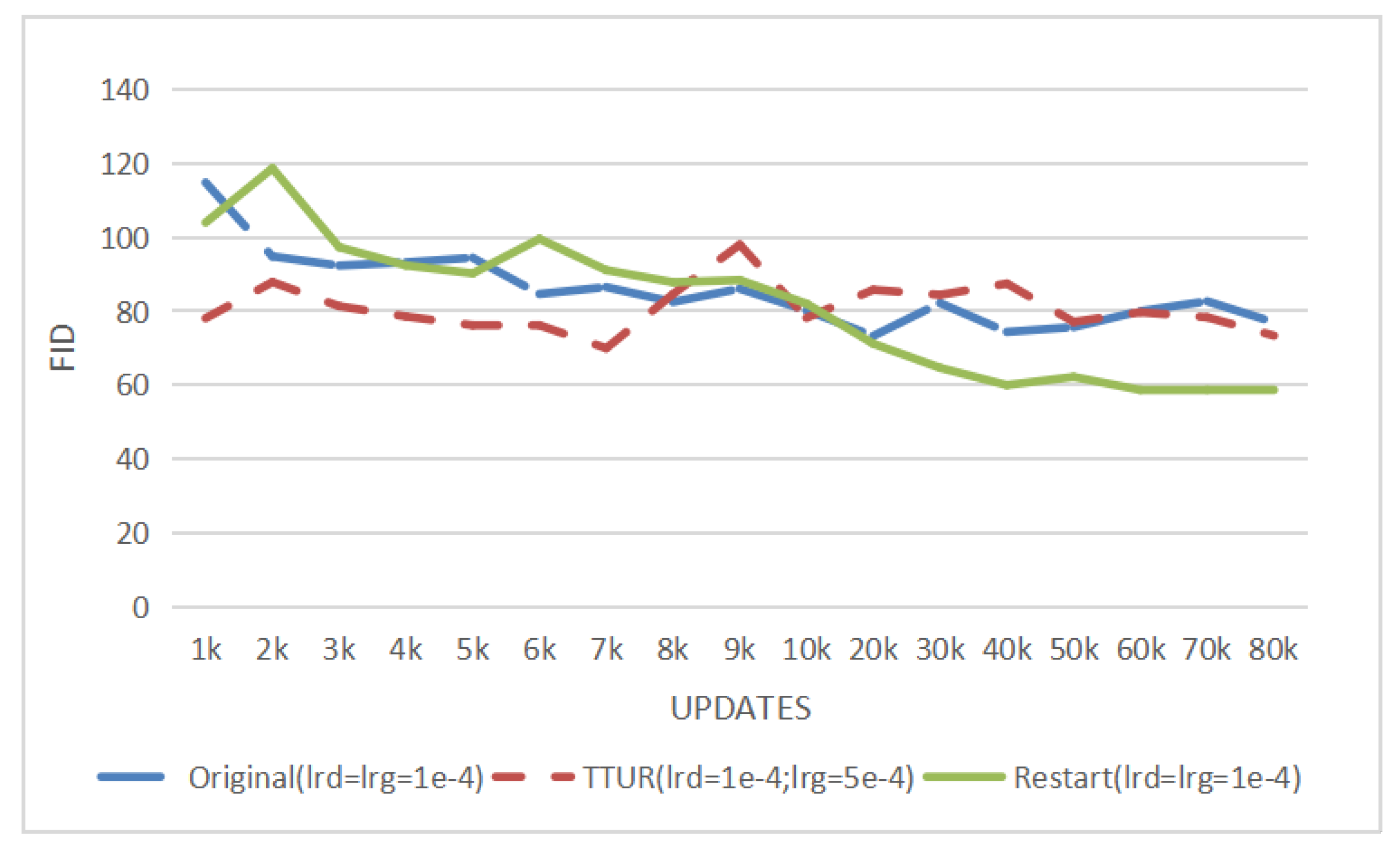
We also compare our method with the Two Time-Scale Update Rule [24]. In Figure 4, ‘Original’ means the DCGAN model in [2], ‘TTUR’ means DCGAN trained by a Two Time-Scale Update Rule [24], and ‘Restart’ means our method proposed in this paper. For fairness, the learning rate and updates settings of Original and TTUR are the same as settings in Table 1 of [24]. In our proposed method (‘Restart’ in Figure 4), the learning rate of the generator is the same as ‘Original’ while the maximum learning rate of the discriminator is also equal to . In Figure 4, compared with the round-trip fluctuation of DCGAN with original learning rates, the FID results indicate that the DCGAN trained with TTUR decreases steadily and outperforms the original DCGAN in 80k updates. However, the DCGAN with our method obtained the highest performance and converges faster than the other two methods.
Figure 4.
FID by DCGAN model on CIFAR-10: Original means the DCGAN model in [2]; TTUR means DCGAN trained by a Two Time-Scale Update Rule [24]; restart means our method proposed in this paper.
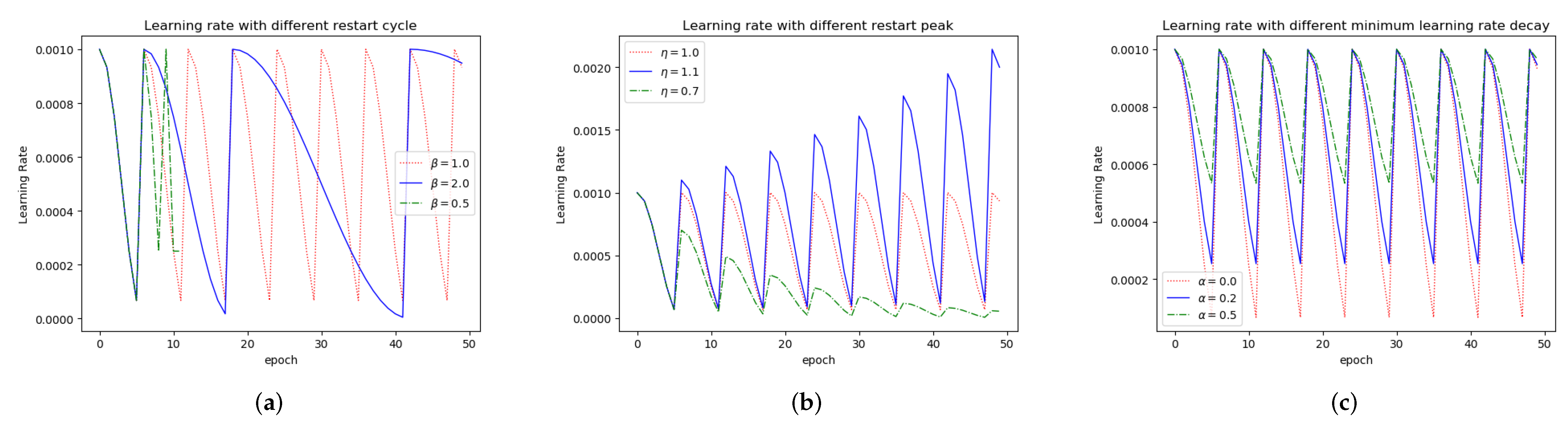
In order to analyze our method in detail, we have further explored the influence of four important parameters in the method on the experiment results and which are shown in the following parts. The four parameters are (cycle length control coefficient), (peak value control coefficient), (the baseline of amplitudes), and P (the number of steps in the first cycle), respectively. As we have discussed in 
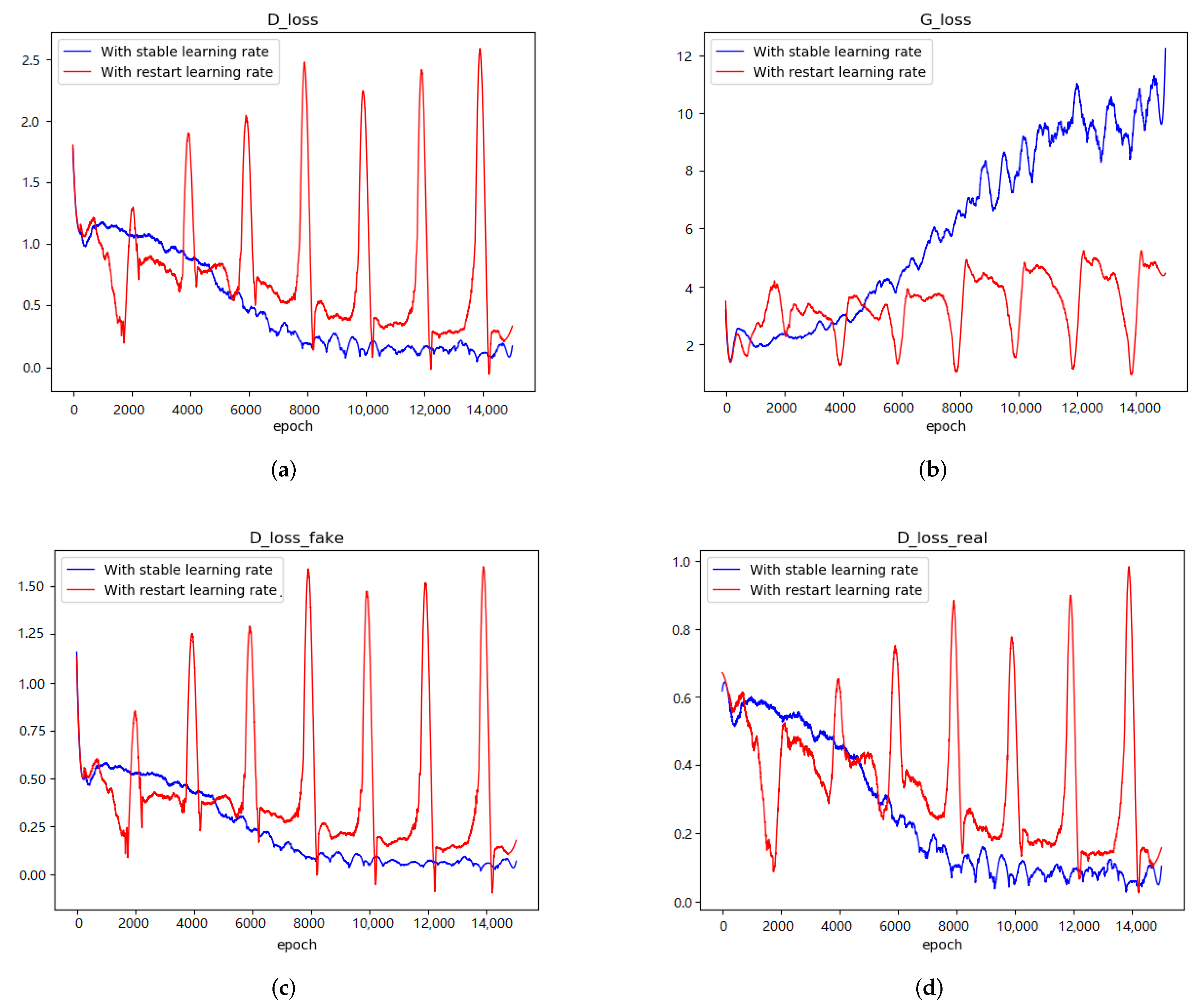
Section 2.2, the line of Figure 1a shows the convergence of D which will influence the final output. Therefore, we have investigated the influence of our method in two ways: (1) the convergence of loss of D and (2) the result in terms of FID. Besides that, we consider the modification of the parameter settings that can prevent the fast convergence of D and ensure the effectiveness during the training process.
In the ablation study of four parameters (, , , and P), we always explore the impact of different values of a parameter when the other three parameters remain unchanged. Based on the analysis of generated results (FID score), we select three representative values to see their impact on the discriminator loss curves.
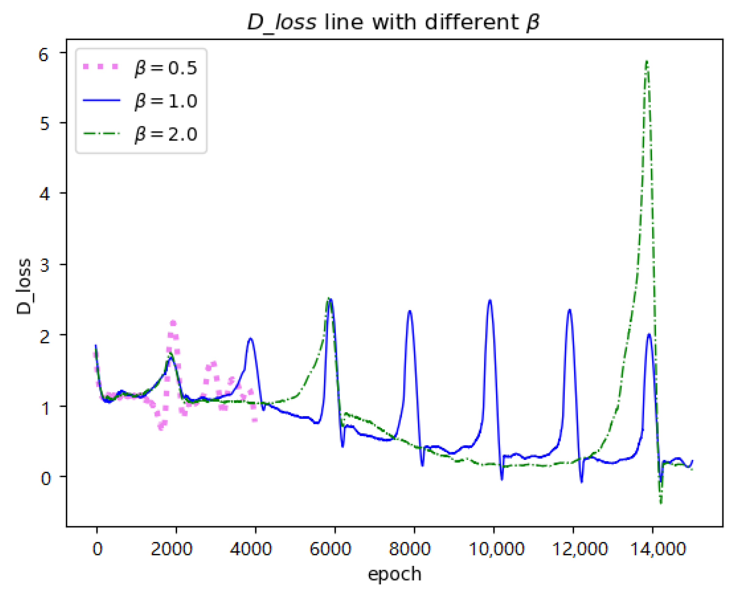
Table 4 gives different values related to the cycle length control coefficient (row 6 in Algorithm 1) and Figure 5 shows three corresponding D loss lines. defines the multiple of the current period length relative to the previous one. According to the update formula of period length (), with a value less than 1.0 (i.e., row 1 in Table 4) shortens the length of a period. When the training process can not run properly, ‘NaN’ situation can occur (pink line in Figure 5). ‘NaN’ represents that the program produces none value. Conversely, a large value (i.e., row 5 and 6 in Table 4) may cause heavy disturbance as shown in the green line of Figure 5 due to the sudden increase of the learning rate in the next period. However, this disturbance will not lead to heavy worse results (i.e., FID score in row 5) because of fast convergence. As shown in Table 4, restart learning rate with performs most effectively (i.e., row 2). However, at the same time, we also note that when we take values between 1.0 and 2.0 for , the differences among them are small (i.e., row 3, row 4, and row 5). Even if is taken as 3.0, the corresponding FID only increases by 3.806 compared with the smallest distance in row 2. In conclusion, we analyze that the value of has little effect on the experimental results, but the values between 1.0 and 2.0 are more conducive for us to obtain satisfying results.
Table 4.
FID results in terms of different . Bold denotes the smallest distance.
Figure 5.
D loss line with different .
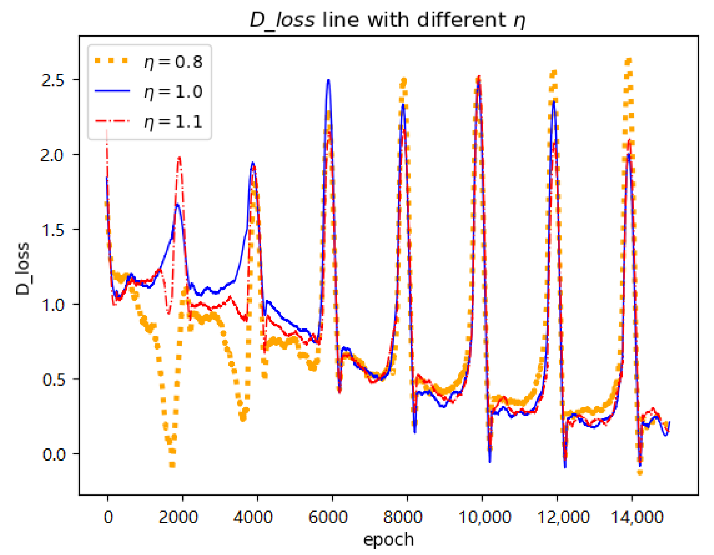
is the multiple of the current peak value relative to the previous one (note line 5 in Algorithm 1). We also set different values to parameter (Table 5). We have observed that makes the peak value cumulative as the epoch increases (orange line in Figure 6), and the increasing fluctuation is not conducive to the convergence of the whole training process. Additionally, larger values lead to worse results (compare row 5 and row 6 in Table 5). However, values set to 1.0 or slightly less than 1.0 are beneficial for generated results (i.e., rows 2,3, and 4). For example, blue line and red line in Figure 6 provide more gentle restart for training process. exhibited the optimal result as shown in the third row of Table 5 (corresponding FID=63.793). In conclusion, we can see that values slightly less than 1.0 are suitable for parameter .
Table 5.
FID results in terms of different . Bold denotes the smallest distance.
Figure 6.
D loss line with different .
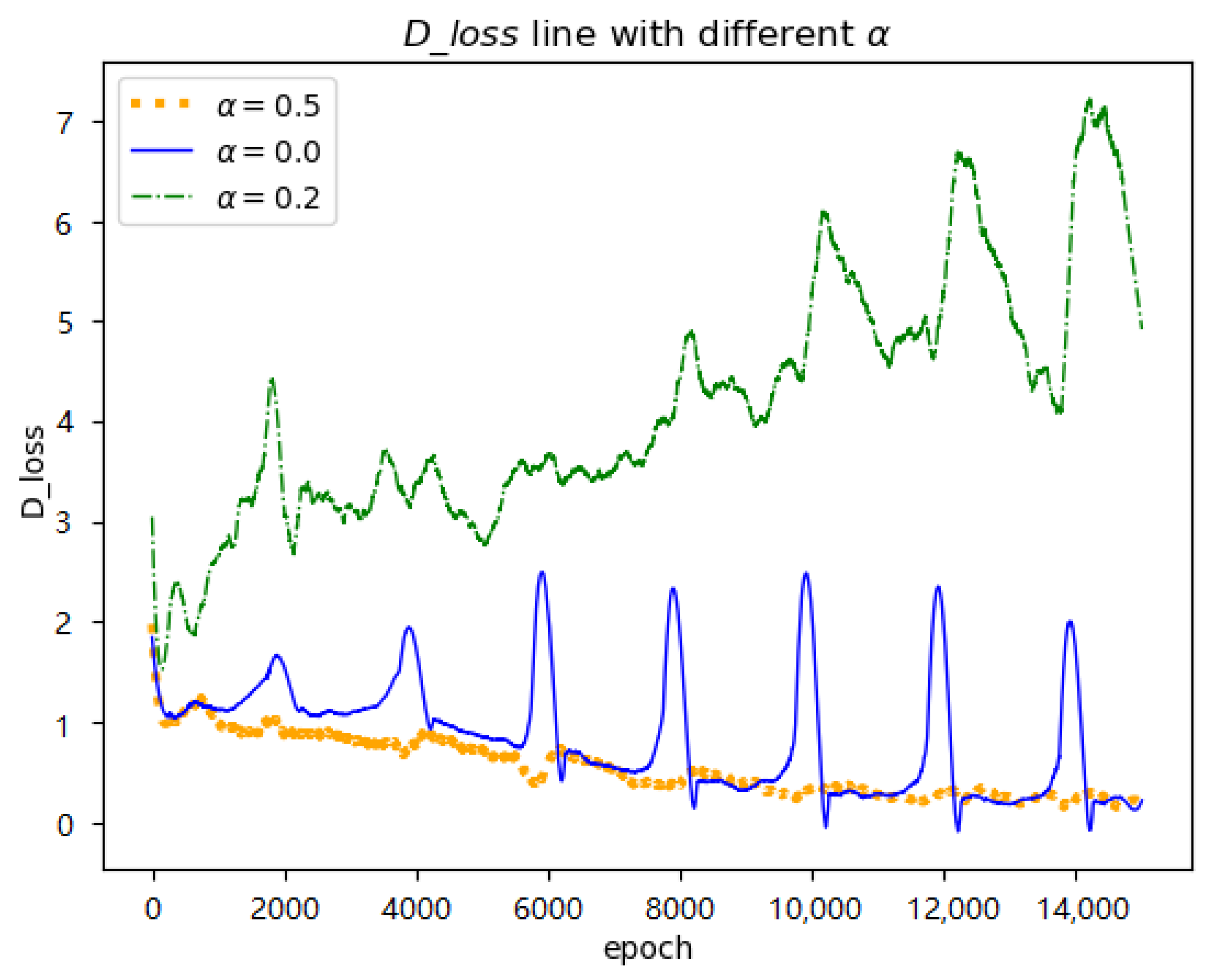
is the minimum value that the learning rate can decay to (shown in line 5 of Algorithm 1). When is 0.0, it means there is no baseline, and the learning rate could decrease to zero to provide no gradient for updating (it is obvious that we need gradients for training GANs). In this way, we set its values between 0.0 and 1.0 to be the baseline of learning rate to explore its impact. When is slightly greater than 0.0, the corresponding generated results are more improved than those of (i.e., row 2, 3, 4 in Table 6). has obtained the optimal performance and the representative line in Figure 7 shows the highest D loss. Thus, the following conclusions can be inferred: appropriate increase D loss can effectively prevent the disappearance of D loss, so as to make GAN generate improved results. However, excessive values can lead to an increase in FID scores (i.e., row 5, 6 in Table 6). Additionally, we also noted that the value makes D loss nearly disappearing (orange line in Figure 7). We conjecture that it is because the range (1.0 to 0.5) of the learning rate is limited, which is contrary to our original intention for restart. All in all, we consider to be most suitable for our method.
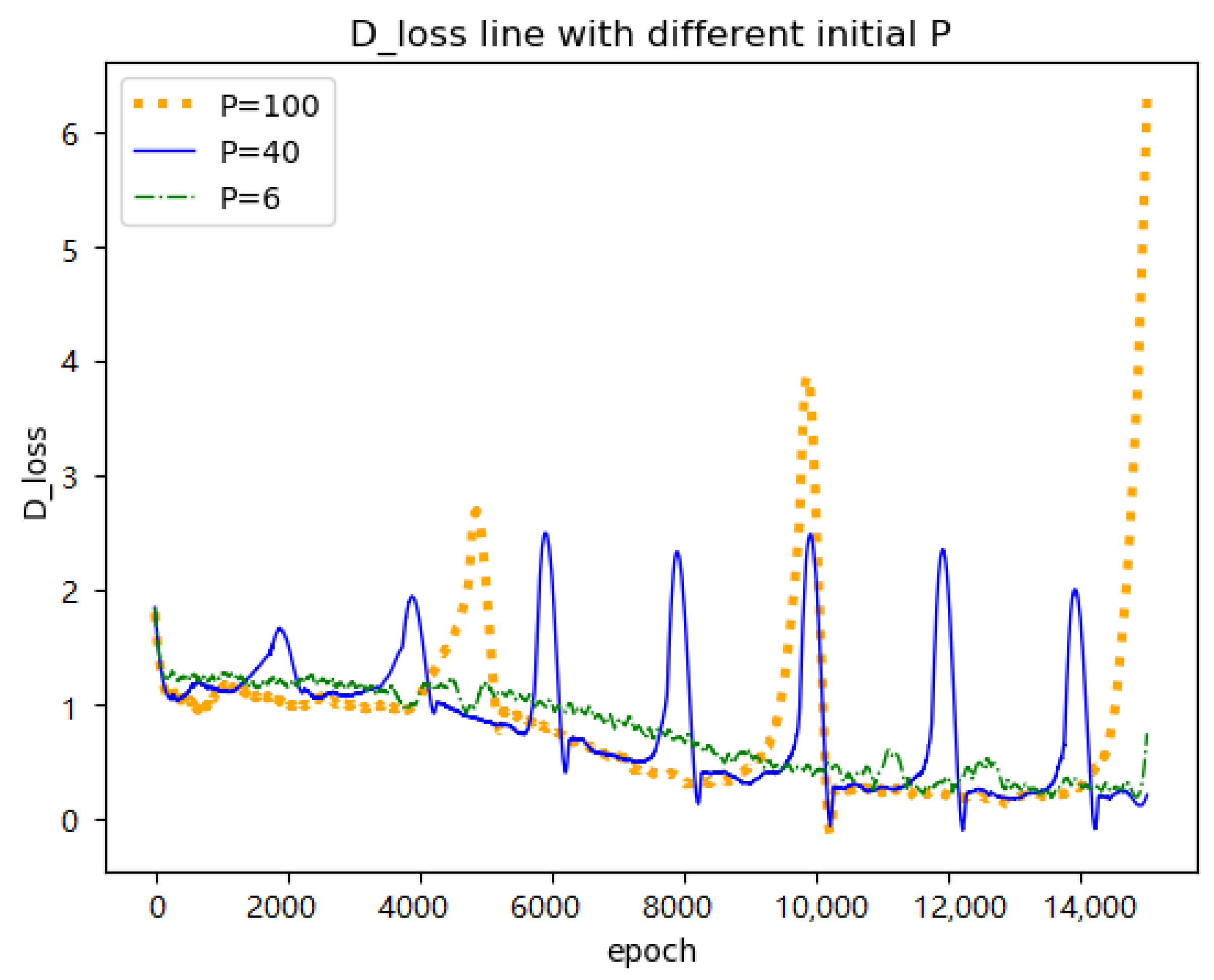
Table 6.
FID results in terms of different . Bold denotes the smallest distance.
Figure 7.
D loss line with different .
P is updated by in the algorithm (line 6 in Algorithm 1). P is the initial number of steps in the first cycle. As was previously discussed, to be 1.0 or slightly greater than 1.0 is a moderate choice for training GANs. Hence too small values of P (i.e., rows 1, 2, and 3 in Table 7) provide limited steps to find potential optima. When the value of P is too large, the period in the loss curve is too long, and the sudden increase of learning rate at the beginning of the next period will bring too high fluctuations to the training process (the orange line in Figure 8). Heavy fluctuation makes the optimization of the previous cycle meaningless which is shown with underperformed generated results (i.e., rows 5 and 6 in Table 7). When the initial value of P is set to 40, it allows the restart learning rate to exercise its full performance and exhibits the satisfactory results (the blue line in Figure 8 and the row 4 in Table 7).
Table 7.
FID results in terms of different initial P. Bold denotes the smallest distance.
Figure 8.
D loss line with different initial P.
Overall, appropriate parameter selection is essential for demonstrating the functionality of our new method. Especially, it is shown that appropriate tuning of and significantly improves the performance. Through various experiments, we found the setting of parameters ( = 1.0, = 0.8, = 0.2, P = 40) which gives satisfiable results. It also could be further explained that remarkable performance corresponds to low FID results. Restart learning prevents the fast disappearance of (Figure 1a) and the rapid growth of (Figure 1b). As explained above, preventing the rapid decline in the loss of the discriminator can effectively improve the performance of GAN, and restarting learning is an effective way for achieving the above-mentioned functions.
5. Conclusions
In this paper, we adopt a restart learning rate in the training of the discriminator. Restarting the learning rate overcomes the problem of the discriminator converging too fast, and the two annealing processes avoid the shock in the later stage of training. Experiments show that restart learning is conducive to GAN’s in-depth mining of data features and improving the quality and diversity of the generated results. This should be the first time restart learning is applied in the training of GAN. Since restart learning only affects the learning rate, this method can be used with other tricks to improve GAN performance.
In the first step of the next research, we want to do more research for the meaningful start which could guide the training track instead of blindly exploring the optimum; secondly, we will try to find the deeper relationship between and the performance of GAN, especially the ; thirdly, further research on saddle problems is necessary; lastly, although FID can evaluate the diversity and quality of the generated results, there is no method to evaluate these two aspects separately, so as to solve the problems of GAN thoroughly.
Author Contributions
Conceptualization, K.L. and D.-K.K.; methodology, K.L.; software, K.L.; validation, K.L. and D.-K.K.; formal analysis, K.L.; investigation, K.L.; resources, K.L. and D.-K.K.; data curation, K.L.; writing—original draft preparation, K.L.; writing—review and editing, D.-K.K.; visualization, K.L.; supervision, D.-K.K.; project administration, D.-K.K.; funding acquisition, D.-K.K. All authors have read and agreed to the published version of the manuscript.
Funding
This research was partly supported by the Technology Development Program “Development of Supply Chain Optimization Technology Based on Big Data and Machine Learning” funded by the Ministry of SMEs and Startups (MSS, Korea) (S3126610) and Doctoral research start-up funds project funded by Weifang University of Science and Technology (China) (2021KJBS12).
Institutional Review Board Statement
Not applicable.
Informed Consent Statement
Not applicable.
Data Availability Statement
Publicly available datasets were analyzed in this study. This data can be found here: [https://www.cs.toronto.edu/~kriz/cifar.html, and https://mmlab.ie.cuhk.edu.hk/projects/CelebA.html] (accessed on 20 October 2021).
Acknowledgments
The authors wish to thank members of the Dongseo University Machine Learning/Deep Learning Research Lab., and anonymous referees for their helpful comments on earlier drafts of this paper.
Conflicts of Interest
The authors declare no conflict of interest.
Abbreviations
The following abbreviations are used in this manuscript:
| GAN | Generative Adversarial Networks |
| GANs | A Series of Generative Adversarial Networks |
| DCGAN | Deep Convolutional Generative Adversarial Networks |
| ProGAN | Progressive Growing of GANs |
| BigGAN | Large Scale GAN |
| SAGAN | Self-Attention GAN |
| StyleGAN | A Style-based Generator Architecture for GAN |
| Sliced WGAN | Sliced Wasserstein Generative Adversarial Networks |
| DNNs | Deep Neural Networks |
| SNGAN | Spectral Normalization for GAN |
| WGAN | Wasserstein GAN |
| WGAN-GP | WGAN with Penalty |
References
- Goodfellow, I.; Pouget-Abadie, J.; Mirza, M.; Xu, B.; Warde-Farley, D.; Ozair, S.; Courville, A.; Bengio, Y. Generative Adversarial Nets. In Advances in Neural Information Processing Systems; Ghahramani, Z., Welling, M., Cortes, C., Lawrence, N., Weinberger, K.Q., Eds.; Curran Associates, Inc.: New York, NY, USA, 2014; Volume 27. [Google Scholar]
- Radford, A.; Metz, L.; Chintala, S. Unsupervised Representation Learning with Deep Convolutional Generative Adversarial Networks. In Proceedings of the 4th International Conference on Learning Representations, ICLR 2016, San Juan, Puerto Rico, 2–4 May 2016. [Google Scholar]
- Arjovsky, M.; Chintala, S.; Bottou, L. Wasserstein Generative Adversarial Networks. In Proceedings of the 34th International Conference on Machine Learning, Sydney, Australia, 6–11 August 2017; Volume 70, pp. 214–223. [Google Scholar]
- Karras, T.; Aila, T.; Laine, S.; Lehtinen, J. Progressive Growing of GANs for Improved Quality, Stability, and Variation. arXiv 2017, arXiv:1710.10196. [Google Scholar]
- Brock, A.; Donahue, J.; Simonyan, K. Large Scale GAN Training for High Fidelity Natural Image Synthesis. In Proceedings of the 7th International Conference on Learning Representations, New Orleans, LA, USA, 6–9 May 2019. [Google Scholar]
- Zhang, H.; Goodfellow, I.; Metaxas, D.; Odena, A. Self-Attention Generative Adversarial Networks. In Proceedings of the 36th International Conference on Machine Learning, Long Beach, CA, USA, 9–15 June 2019; Volume 97, pp. 7354–7363. [Google Scholar]
- Karras, T.; Laine, S.; Aila, T. A Style-Based Generator Architecture for Generative Adversarial Networks. In IEEE/CVF Conference on Computer Vision and Pattern Recognition (CVPR); IEEE: Piscataway, NJ, USA, 13–15 February 2019; pp. 4396–4405. [Google Scholar] [CrossRef] [Green Version]
- Wu, J.; Huang, Z.; Acharya, D.; Li, W.; Thoma, J.; Paudel, D.P.; Gool, L.V. Sliced Wasserstein Generative Models. In Proceedings of the IEEE/CVF Conference on Computer Vision and Pattern Recognition (CVPR), Long Beach, CA, USA, 16–20 June 2019. [Google Scholar]
- Miyato, T.; Kataoka, T.; Koyama, M.; Yoshida, Y. Spectral Normalization for Generative Adversarial Networks. arXiv 2018, arXiv:1802.05957. [Google Scholar]
- Lucic, M.; Kurach, K.; Michalski, M.; Gelly, S.; Bousquet, O. Are GANs Created Equal? A Large-Scale Study. In Advances in Neural Information Processing Systems; Bengio, S., Wallach, H., Larochelle, H., Grauman, K., Cesa-Bianchi, N., Garnett, R., Eds.; Curran Associates, Inc.: Montréal, QC, Canada, 3–8 December 2018; Volume 31. [Google Scholar]
- Mescheder, L.; Geiger, A.; Nowozin, S. Which Training Methods for GANs do actually Converge? In Proceedings of the 35th International Conference on Machine Learning, Stockholm, Sweden, 10–15 July 2018; Dy, J., Krause, A., Eds.; Stockholmsmässan: Stockholm, Sweden, 2018; Volume 80, pp. 3481–3490. [Google Scholar]
- Kurach, K.; Lucic, M.; Zhai, X.; Michalski, M.; Gelly, S. A Large-Scale Study on Regularization and Normalization in GANs. arXiv 2019, arXiv:1807.04720v3. [Google Scholar]
- Arjovsky, M.; Bottou, L. Towards Principled Methods for Training Generative Adversarial Networks. In Proceedings of the 5th International Conference on Learning Representations, ICLR 2017, Toulon, France, 24–26 April 2017; Available online: OpenReview.net (accessed on 20 October 2021).
- Bińkowski, M.; Sutherland, D.J.; Arbel, M.; Gretton, A. Demystifying MMD GANs. arXiv 2018, arXiv:1801.01401. [Google Scholar]
- Roth, K.; Lucchi, A.; Nowozin, S.; Hofmann, T. Stabilizing Training of Generative Adversarial Networks through Regularization. arXiv 2017, arXiv:1705.09367. [Google Scholar]
- Wang, B.; Nguyen, T.M.; Bertozzi, A.L.; Baraniuk, R.G.; Osher, S.J. Scheduled Restart Momentum for Accelerated Stochastic Gradient Descent. arXiv 2020, arXiv:2002.10583. [Google Scholar]
- Smith, L.N. Cyclical Learning Rates for Training Neural Networks. In Proceedings of the 2017 IEEE Winter Conference on Applications of Computer Vision (WACV), Santa Rosa, CA, USA, 24–31 March 2017; pp. 464–472. [Google Scholar] [CrossRef] [Green Version]
- Loshchilov, I.; Hutter, F. SGDR: Stochastic Gradient Descent with Warm Restarts. In Proceedings of the 5th International Conference on Learning Representations, ICLR 2017, Toulon, France, 24–26 April 2017; Available online: OpenReview.net (accessed on 20 October 2021).
- Huang, G.; Li, Y.; Pleiss, G.; Liu, Z.; Hopcroft, J.E.; Weinberger, K.Q. Snapshot Ensembles: Train 1, Get M for Free. In Proceedings of the 5th International Conference on Learning Representations, ICLR 2017, Toulon, France, 24–26 April 2017; Available online: OpenReview.net (accessed on 20 October 2021).
- Li, X.; Xiong, H.; An, H.; Xu, C.Z.; Dou, D. RIFLE: Backpropagation in Depth for Deep Transfer Learning through Re-Initializing the Fully-connected LayEr. In Proceedings of the 37th International Conference on Machine Learning, Online, 12–18 July 2020; Volume 119, pp. 6010–6019. [Google Scholar]
- Dauphin, Y.N.; Pascanu, R.; Gulcehre, C.; Cho, K.; Ganguli, S.; Bengio, Y. Identifying and Attacking the Saddle Point Problem in High-dimensional Non-convex Optimization. In Advances in Neural Information Processing Systems; Ghahramani, Z., Welling, M., Cortes, C., Lawrence, N., Weinberger, K.Q., Eds.; Curran Associates, Inc.: Iguassu Falls, Brazil, 8–13 December 2014; Volume 27. [Google Scholar]
- Kingma, D.P.; Ba, J. Adam: A Method for Stochastic Optimization. arXiv 2014, arXiv:1412.6980. [Google Scholar]
- Gulrajani, I.; Ahmed, F.; Arjovsky, M.; Dumoulin, V.; Courville, A. Improved Training of Wasserstein GANs. arXiv 2017, arXiv:1704.00028. [Google Scholar]
- Heusel, M.; Ramsauer, H.; Unterthiner, T.; Nessler, B.; Hochreiter, S. GANs Trained by a Two Time-Scale Update Rule Converge to a Local Nash Equilibrium. In Advances in Neural Information Processing Systems; Guyon, I., Luxburg, U.V., Bengio, S., Wallach, H., Fergus, R., Vishwanathan, S., Garnett, R., Eds.; Curran Associates, Inc.: Long Beach, CA, USA, 4–9 December 2017; Volume 30. [Google Scholar]
Publisher’s Note: MDPI stays neutral with regard to jurisdictional claims in published maps and institutional affiliations. |
© 2022 by the authors. Licensee MDPI, Basel, Switzerland. This article is an open access article distributed under the terms and conditions of the Creative Commons Attribution (CC BY) license (https://creativecommons.org/licenses/by/4.0/).