Article

Anomaly Monitoring of Process Based on Recurrent Timeliness Rules (AMP-RTR)

1
College of Computer Science, Sichuan University, Chengdu 610065, China
2
Big Data Analysis and Fusion Application Technology Engineering Laboratory of Sichuan Province, Chengdu 610065, China
*
Author to whom correspondence should be addressed.
Appl. Sci. 2022, 12(24), 12917; https://doi.org/10.3390/app122412917
Submission received: 4 November 2022 / Revised: 12 December 2022 / Accepted: 13 December 2022 / Published: 15 December 2022
(This article belongs to the Special Issue IIoT-Enhancing the Industrial World and Business Processes)

Abstract

:
At present, many manufacturing enterprises have business systems such as MES, SPC, etc. In the manufacturing process, a large amount of data with periodic time series will be generated. How to evaluate the timeliness of periodically generated data according to a large number of time series is important content in the field of data quality research. At the same time, it can solve the demand of abnormal monitoring of production process faced by manufacturing enterprises based on the regularity change for periodic data timeliness. Most of the existing data timeliness evaluation models are based on a single fixed time stamp, which is not suitable for effective evaluation of periodic data with time series. In addition, the existing data timeliness evaluation methods cannot be applied to the field of process anomaly monitoring. In this paper, the Anomaly Monitoring of Process based on Recurrent Timeliness Rules (AMP-RTR) is proposed to meet the needs of periodic data timeliness evaluation and production process anomaly monitoring. RTR is the Rules defined to evaluate the timeliness of periodically generated data. AMP is to infer the abnormality of the product production process through the abnormality of the regularity change for periodic data timeliness based on RTR. The AMP-RTR model evaluates the timeliness of data in each cycle according to the time series generated periodically. At the same time, after the updated data arrives, the initial timeliness score of the next cycle is calculated. There are two cases in which the evaluation value of timeliness is abnormal. The first case is that the timeliness score value is less than the lower limit after updating. The second case is that the number of times the timeliness score exceeds the upper limit meets the set threshold. The user can dynamically adjust the production process according to the abnormal warning of the model. Finally, in order to verify the applicability of the AMP-RTR, we conducted simulation experiments on synthetic datasets and semiconductor manufacturing datasets. The experimental results show that the AMP-RTR can effectively monitor the abnormal conditions of various production processes in the manufacturing industry by adjusting the parameters of the model.

1. Introduction

As the manufacturing industry becomes more and more intelligent, a large number of sensors will collect various types of data in the process of workpiece production. Different from the traffic data on the Internet, the data generated by the manufacturing industry are often structured, cyclical and with a clear timestamp. These data collected by various types of sensors contain valuable information about each production entity. Using these data, we can obtain knowledge about the output of the production line, the faults occurred and their results, as well as many other information vital to the operation of the plant. The quality of these data needs to be assessed before they can be used. The timeliness of data is an important dimension of data quality [1], so how to evaluate the timeliness of cyclical manufacturing data is very critical. However, the existing data timeliness evaluation methods cannot effectively evaluate periodic data. In addition, anomaly monitoring in manufacturing industry is usually realized by data mining and pattern matching, without considering the dimension of time [2]. Therefore, we propose an Anomaly Monitoring of Process based on Recurrent Timeliness Rules (AMP-RTR). The model can not only effectively evaluate the timeliness of periodic data, but also find the anomalies in the production process by monitoring the regularity change for periodic data timeliness.

1.1. Definition of Data Timeliness

The definition of most data timeliness is that as long as data meets the needs of work, it is effective. In addition, the premise of most data timeliness definitions is to store data correctly. Compared with the correctness of data, the timeliness of data does not necessarily need to be tested in the real world. Accordingly, the measurement of data timeliness should be an estimate rather than a verification statement under certainty (which is necessary for correctness) to determine the probability that the value of data attributes is still up-to-date. The literature [3,4] interprets timeliness as the probability that relevant data are still valid. For a large amounts of data, when the recurrent validity of the data is not clear, it seems reasonable to quantify timeliness through this estimation. This is because comparing attribute values with their real-world counterparts (real-world tests) usually takes a lot of time, which is neither economical nor realistic [5].

1.2. Characteristics of Manufacturing Data

Manufacturing big data is the core of intelligent manufacturing. Based on “big data and industrial Internet of Things”, cloud computing, big data, Internet of Things, artificial intelligence and other technologies are used to lead the transformation of industrial production methods and drive the innovative development of industrial economy. In addition to the characteristics of general big data (volume, variety, velocity, value), manufacturing big data also has the characteristics of sequence, strong relevance, accuracy and closed-loop. The essential characteristic of manufacturing data is the complex dynamic system. Certainty is the basis for the effective operation of industrial systems. The premise of dealing with uncertainty is anomaly monitoring and eliminating uncertainty. As factories become more and more intelligent, smart interconnected products embedded with sensors have become an important symbol of the industrial Internet era. These sensors will periodically collect various data in the production process. The generation of these data is often periodic and has a clear time stamp. Therefore, a regular time series will be formed.

1.3. Paper Organization and Contribution

The guiding principles of designing scientific research defined in reference [6], we regard the recurrent timeliness Rules as our artifact, and organize the paper as follows: after discussing the relevance of the problems in this introduction, Section 2 briefly summarizes the relevant work on data timeliness, and identifies the research gap. Our contribution is to propose the Anomaly Monitoring of Process based on Recurrent Timeliness Rules, which infers the abnormality of the production process according to the abnormality of the timeliness score. In Section 3, based on the previous work and the actual needs of manufacturing production, we first summarized the requirements for Recurrent Timeliness Rules. Then, the evaluation method of the timeliness of periodic data and the realization of the process anomaly monitoring model are introduced, respectively. In Section 4, we first tested the robustness of the model on synthetic datasets, and then carried out simulation experiments on the semiconductor manufacturing datasets. In Section 5, we summarize the advantages of this model over the existing methods and look forward to the research points that can be optimized in the future.
Figure 1 summarizes the ideas of this research work. The AMP-RTR research flow chart divides the research content of this paper into two main aspects: one is the iterative process for the timeliness evaluation of periodic data (i.e., RTR), and the other is the implementation process of anomaly monitoring (i.e., AMP). This figure clearly shows how the timeliness evaluation achieves iterative updating, and how to realize the abnormal monitoring and feedback of the production line.
The possible contributions of this paper are as follows:
(1)
The current data timeliness evaluation method is based on a single timestamp in the database and cannot evaluate the timeliness of periodic data with time series. Therefore, according to the characteristics of periodic production of manufacturing data, we propose the Recurrent Timeliness Rules (RTR). RTR define the basis for regularity change of periodic data timeliness; that is, how the regularity change of periodic data timeliness occurs during the update cycle, and how the regularity change of periodic data timeliness is updated iteratively. According to RTR’s constraints on the regularity change for periodic data timeliness, the timeliness evaluation of periodic data can be realized.
(2)
According to the regularity change for periodic data timeliness, we propose the Anomaly Monitoring of Process based on Recurrent Timeliness Rules (AMP-RTR). At the same time, we specified two cases of abnormal changes in the regularity change for periodic data timeliness: the first abnormal state is that the timeliness evaluation value is lower than the lower limit after updating; the second abnormal state is that the number of times the timeliness evaluation value is higher than the upper limit reaches the set threshold after being updated. AMP-RTR model monitors whether the update iteration of regularity change of periodic data timeliness is abnormal, so as to calculate the possibility of abnormality in the production line. The model adjusts the decay rate f a l l   A and periodic update rate α , so as to meet the customized requirements for monitoring sensitivity of different production lines in the manufacturing industry.

2. Related Work

There are many well-known and important contributions to data timeliness assessment and they are also used in many real-world scenarios. First, we discuss the existing contributions from the perspective of timeliness of the data quality dimension. Then, we summarize the application scenarios of the existing timeliness evaluation methods. Finally, we determine the research direction according to the actual needs of the manufacturing industry.
There are many different terms in the field of representing data timeliness: currency, timeliness, staleness, up-to-date, freshness, temporal validity. In the area of data timeliness, Ballou et al. [7] was one of the earliest and most famous contributions. They define a measure as a function that depends on the age of the attribute value at the time the currency is evaluated, the (fixed and given) shelf life of the attribute value, and the sensitivity parameters that make the measure suitable for the application environment. The value of this indicator depends on the average frequency with which attribute values (approximately) are updated in practice and the time elapsed from the moment the currency is evaluated to the time the attribute values are obtained. Even and Shankaranarayanan [8] propose another indicator in terms of functions that depend on the length of time between the moment the currency is evaluated and the moment the attribute value is obtained ( t 1 t 0 ) or updated or confirmed ( t 1 t 0 ). The main idea of their approach is to map measures across 0 1 , where a value of 1 represents a perfectly good currency and a value of 0 represent a totally bad currency. Li et al. [9] used volatility as an index of an exponential function that multiplies as a proportion factor of money, and volatility is the probability that data will be updated over time. Heinrich and Klier [10] proposed a measure based on conditional expectation and additional metadata, which produces interpretable and interval scaled measures. The classification methods used include support vector machines [11,12,13] and logistic regression [14] to deep neural networks [15]. All the above-mentioned authors have proposed a metric for currency in a general environment, and there are no specific scenarios. Of course, a lot of attempts and contributions have been made by predecessors in the field of data timeliness application. Heinrich, Bernd and Klier [16] applied the timeliness index to a German financial service provider (FSP) to support the valuation of customers. Otmane [17] describes how to evaluate the data timeliness described in the literature in the research information system (RIS). Heinrich and Klier [18], by quantifying the timeliness of the data quality dimension, implemented efficient Customer Relationship Management (CRM) for the activities of a large mobile service provider. Klier and Matthias [19] apply probability-based data currency assessment methods and event-driven mechanisms to reflect the likelihood that Wikipedia articles are still up-to-date (that is, no currency-related events change the state of the corresponding entity), so they can distinguish between current and past articles very well. Khalil Ibrahimi et al. [20] explained the time impact through seasonal autoregressive comprehensive moving average (SARIMA) based on the time series model, and proposed a scheme to predict the popularity and evolution of video content. Reinier Torres Labrada [21] proposed an exception detection framework MuSADET for timing exceptions found in real-time embedded system event tracking. MuSADET compares the frequency domain characteristics of the unknown trajectory with the normal model trained from the good execution of the system. This method uses static event generator, signal processing and distance measurement to classify the time series between arrivals as normal/abnormal, which can better detect the system exceptions. The A A R D (Average Absolute Relative Deviations) method proposed by B Rajarayan Prusty et al. [22] can better measure the outlier of data through the true positive (TP) and false positive (FP) of the known outlier information. However, the existing methods are not suitable for the large amount of data generated recurrently in the actual production process of the manufacturing industry. At the same time, data timeliness evaluation has not been applied in the manufacturing industry, especially in industrial production process monitoring.
To sum up, predecessors have achieved a lot of work on data timeliness. These works include putting forward a general timeliness evaluation model and applying it to many practical scenarios. However, when these methods are directly applied to the manufacturing industry, their applicability will be hindered. First of all, these methods do not consider the time series generated by multiple production lines and products in the manufacturing industry. Secondly, these methods simply input the time of data generation into the model as a parameter. The relative stability of the data generated in the manufacturing industry is not considered. Finally, the timeliness evaluation of data has not been applied in the field of anomaly monitoring.

3. Design of AMP-RTR Model

3.1. Metric Requirements of AMP-RTR Model

In order to develop the Anomaly Monitoring of Process based on Recurrent Timeliness Rules (AMP-RTR), we propose four main indicators according to the existing literature [7,8,18,23,24,25] and the actual situation of the manufacturing industry, which can be summarized as follows:
R1 (normalization): The data update time of product attributes usually has different periodic, and the data update periodic of different attributes may vary greatly. However, the length of the update cycle is not directly related to the timeliness of the data, so it is necessary to standardize the update cycle according to different application scenarios. The time series can be normalized to twice the set period. For example, when the period T = 7 is set, the time series can be normalized to 0 14 .
The sequence T = t 1 , t 2 , t 3 , , t k is normalized to a b .
t z i = a + b a × t i min T M a x T min T
R2 (interval scale): In order to make the difference between the timeliness scores updated by the two iterations meaningful, we require the iteration to adopt interval scale. For example, the change of timeliness score value from 0.8 to 0.6 at the beginning of the recurrent update should indicate the same degree of data timeliness attenuation compared with the change from 0.6 to 0.4. At the same time, the timeliness score value iterating from 0.6 to 0.7 should represent the same degree of data timeliness improvement as that iterating from 0.5 to 0.6.
R3 (interpretability): The process monitoring alarm must be easy to understand and allow users to effectively find abnormal conditions. In other words, the Anomaly Monitoring of Process on the Recurrent Timeliness Rules (AMP-RTR) issues an abnormal warning, which should indicate that there is a high probability of an anomaly in the product production process. On the contrary, if the AMP-RTR model method does not monitor abnormalities (i.e., does not remind the user), it should indicate that the product production process has no abnormalities in a high probability.
R4 (availability): In the manufacturing process, a large amount of data will be generated recurrently. It must be ensured that the time series of data updates can be transmitted to the processor timely and accurately. At the same time, the processor can effectively process the time series and feedback the processing results to the user in time.

3.2. Implementation of AMP-RTR Model

It must be ensured that the timeliness score meets the normalization (R1) and interval scaling (R2) in each recurrent update of the data, and make the monitoring model interpretable (R3) and effective (R4). According to the timeseries generated in the production process, we propose the Anomaly Monitoring of Process based on Recurrent Timeliness Rules (AMP-RTR). Its core idea is to calculate the timeliness evaluation value of data in each recurrent update of data, and update the timeliness score value iteratively with the recurrently updated data.

3.2.1. Timeliness Evaluation Process of Periodic Data
The Recurrent Timeliness Rules (RTR) defines the attenuation function of the regularity change for periodic data timeliness in the process of data iteration and update. We effectively evaluate the timeliness of periodic data according to RTR.
We assume that at the beginning of the first cycle, the score based on the Recurrent Timeliness Rules is 1. In each cycle, the timeliness score of the data decreases exponentially until the updated data of the next cycle arrives. The principle of regularity change for periodic data timeliness can be summarized as follows: first, if the data update time is equal to the set cycle, the updated timeliness evaluation value is equal to the initial timeliness evaluation value of the current cycle; second, if the time when the data are updated is earlier than the set cycle, the updated timeliness evaluation value should be greater than the initial timeliness evaluation value of the current cycle; third, if the time when the data are updated is later than the set cycle, the updated timeliness evaluation value should be less than the initial timeliness evaluation value of the current cycle.
When the data update frequency is equal to a predetermined period (the error is less than one unit after removing the dimension), the updated timeliness score value is equal to the initial timeliness score value of the current period.
f n + 1 t , λ | A = f n t , λ | A
The f n + 1 t , λ | A is the initial timeliness score of the next cycle after updating. f n t , λ | A is the initial timeliness score of the current cycle. When the update time of data is earlier or later than the set period, the iterative update rule can be expressed by the following formula:
f n + 1 t , λ | A = f n t , λ | A + α × Q d e c a y ( t , λ | A )
The α is the cycle update rate (it should be set reasonably, usually a relatively small value). Q d e c a y ( t , λ | A ) is the timeliness score after attenuation at the end of this week. From Formula (3), we can see that the aging score value after attenuation in the cycle multiplied by the periodic update rate, plus the initial aging score value of the current cycle will be taken as the aging score value of the updated data. The Q d e c a y ( t , λ | A ) value is positive when the time of data update is earlier than the set period, and negative when the time of data update is later than the set period. The highest score of data timeliness is 1. If the updated timeliness score is greater than 1, it will be reset to 1. This principle should be followed when calculating the initial score of each recurrent update of data.
In each updated cycle of the data, we assume that the timeliness score of the data always decays exponentially with time. Exponential distribution is a typical life probability distribution, which has been proved to be very useful in quality management [3]. Therefore, in each update cycle, the evaluation value of data timeliness can be calculated by Formula (7).
Q d e c a y t , λ | A = 1 t T l i f e × e f a l l A a g e t , λ
It is assumed that the law of decline of score values obey exponential decay. A is a data attribute (e.g., temperature), f a l l A indicates the decay rate of the attribute value that expires within a time cycle. For example, the value of f a l l A = 0.2 must be interpreted as follows: on average, 20% of the value of attribute A loses its validity over a cycle of time. a g e t , λ is a function of time t , which indicates the time that the data may change. When a g e t , λ = 0 , Q d e c a y ( t , λ | A ) = 1 ; when a g e = T l i f e , Q d e c a y ( t , λ | A ) = 0 . The definition also complies to the general principle that when the attribute will not change at all, for example, date of product code, for which f a l l A = 0 and T l i f e , the Q d e c a y t , λ | A is always 1 [9].
In the process of product production, the product attribute data will remain constant for a period of time after each periodic update. The frequency of changes in empirical or statistical data is λ , meaning that we expect it to update λ times in a regularization period (it can be a day or a second). The value of λ is usually smaller than the set data update frequency. We can calculate the reasonable existence time of the data through the following formula:
a g e t , λ = 0 t P P r o b a b i l i t y   o f   c h a n g e   a t   x × t x d x .  
The t x indicates the time from possible data changes to monitor: We assume that we evaluate the data at time t and the data are changed at time x . We multiply it by the probability that the data may occur at time x . Relevant research shows that the change of data obeys Poisson distribution, which means that the time until the next change is governed by an exponential distribution [26]. This provides us with a Formula (8) for inserting the P P r o b a b i l i t y   o f   c h a n g e   a t   x expression.
a g e t , λ = 0 t λ e λ x × t x d x
Time t represents the relative time in a cycle (the value of t in each data cycle returns to zero). Before calculation, t must be normalized to eliminate the influence of different dimensions. That is to say, if the dimension of periodic update of data is days, the measurement unit of t should be days. Similarly, when the cycle is updated in seconds, t should be measured in seconds. For example, when the data update cycle of the product is 7 s, the dimension of t should be 1 s. Finally, in order to better apply to the exponential decay law of the model, the value of t should not be too large (usually less than 10).
We evaluate the timeliness of the data generated periodically. There are two main reasons why we use a g e t , λ instead of time t as the timeliness evaluation factor. Firstly, in the actual manufacturing process, the data value will be stable for a short period of time after each update. For example, the temperature and humidity of the updated workpiece will remain unchanged for a short time. Therefore, it is reasonable to choose the time point for evaluating timeliness after this steady state. Secondly, since a g e t , λ is used as the variable of the timeliness evaluation function, the advantage of this is to passivate the time t . In this way, the change trend of timeliness evaluation function is more stable, and the iterative process of timeliness score value is smoother, so as to realize process anomaly monitoring more accurately.
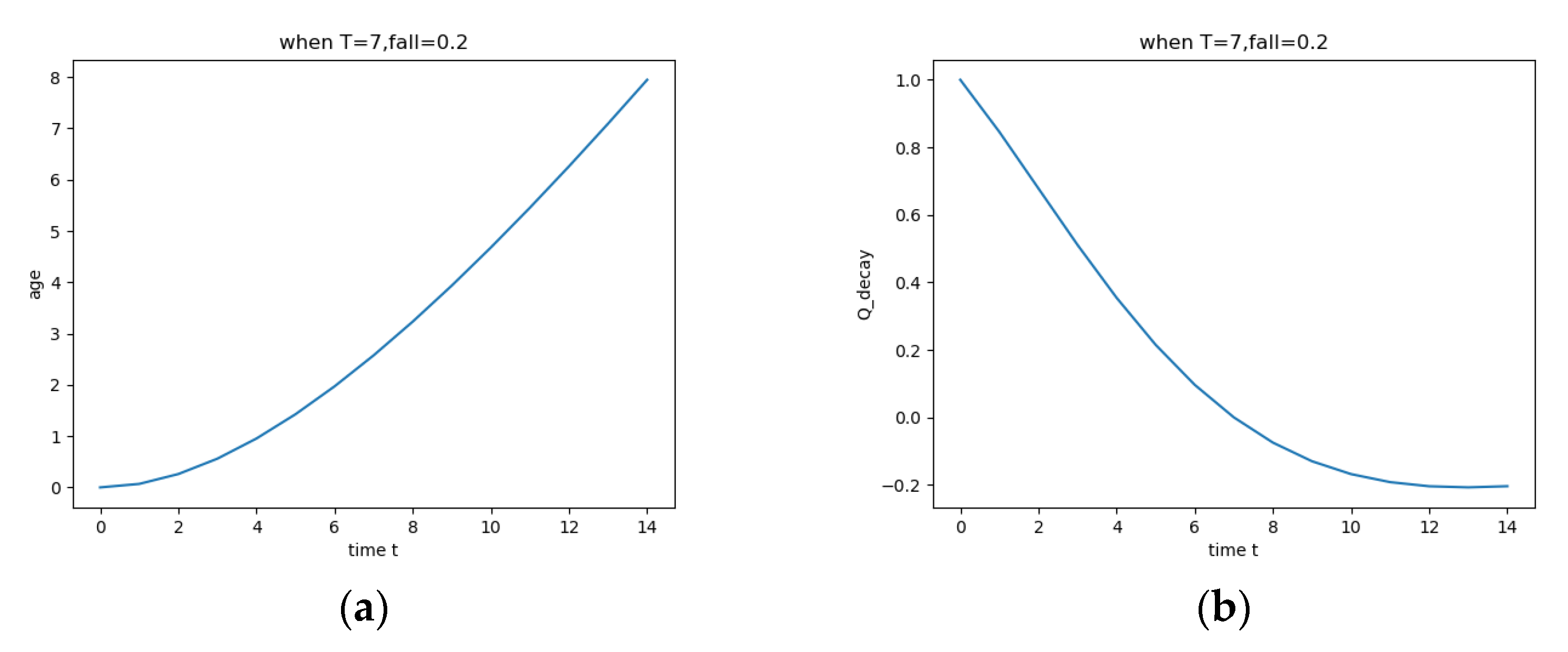
Figure 2 shows the change trend of the two expressions when T = 7 . Indicates the change trend of Q d e c a y t , λ | A and a g e with time T before the arrival of updated data. As you can see from the Figure 2a, the expected a g e t , λ rises slowly and then rapidly. This is because data changes are unlikely to occur in a short period of time after periodic updates. Over time, the possibility of data changes increases rapidly. Since a g e t , λ is used as the factor of the timeliness evaluation function, the change trend of the timeliness score of the data in an update cycle is relatively flat, as is shown Figure 2b.
Figure 2. Trend of expected a g e and timeliness score of data with t ( T = 7 ).
Applsci 12 12917 g002
In Figure 2, the x-axis t i m e   t represents the time value after dimension removal by interval. The y-axis a g e in (a) represents the probability duration after dimension removal obtained according to the method of updating strategy [26]. The y-axis Q _ d a c a y in (b) represents the timeliness score of a data update cycle.

3.2.2. Anomaly Monitoring of Process

Abnormal monitoring shall be conducted for the regularity change of periodic data timeliness. We define two types of monitoring exceptions: the number of records R A reaches the set threshold N A and the updated score is less than 0. The user dynamically adjusts the production line according to the type of abnormal warning.
There are two main reasons for the definition of these two types of asymmetric anomalies: first, the attenuation change of the timeliness evaluation value is not linear, so the iterative update of the timeliness evaluation value is not asymmetric when the deviation before and after the set cycle is the same. Second, the evaluation value of timeliness always declines from the upper limit during the update cycle, and it is not suitable to use exceeding the upper limit as the judgment basis for anomalies. The periodic update rate α in Formula (3) controls the sensitivity of model anomaly monitoring. Users can adjust the sensitivity requirements of abnormal monitoring according to different production lines. If the periodic update rate α is set too high, the sensitivity of the monitoring model will be too high (there is a possibility of false alarm). Conversely, if the periodic update rate α is set too small, the sensitivity of the monitoring model will be too low (unable to meet the needs of monitoring). Those whose updated timeliness score is greater than 1 is recorded. When the recorded value R A meets the set threshold N A (its value can be set as shown in Formula (10)), the user shall be warned in time. Accordingly, when the time of data update is later than the set cycle, the initial score value for the next cycle should be equal to the initial score value for this cycle plus the cycle update rate multiplied by the attenuated value Q d e c a y t , λ | A (when the data are updated later than the preset cycle, the value should be negative) in the cycle, the user shall be warned in time. The specific implementation flow is shown in Figure 3.
Formula (3) is the iterative update of the timeliness score value when only one attribute (such as the timeseries of temperature) is considered. When multiple attributes (such as temperature, humidity, pressure, flow, etc.) need to be considered, the calculation method of iterative update of timeliness score value is as shown in Formula (7).
f n + 1 1 f n + 1 2 f n + 1 3 f n + 1 k = f n 1 f n 2 f n 3 f n k + α 1 , a 2 , α 3 , , α k × Q A 1 Q A 2 Q A 3 Q A k
When considering the timeseries of multiple attributes, the timeliness score value is iteratively updated by Formula (7). Determine a matrix according to the requirements of different attributes of products on monitoring sensitivity. The higher the sensitivity of an attribute to anomaly monitoring, the greater the value of α .
f m i n = min f n + 1 1 , f n + 1 2 , f n + 1 3 , , f n + 1 k < 0 S t o p
After each iteration update, the smallest score value is selected according to Formula (8), and it is judged whether its value is less than 0.
R A 1 N A 1 R A 2 N A 2 R A k N A k S t o p
As shown in Formulas (8) and (9), there are two cases in which the model iteration ends. First, the value of f m i n is less than 0. Second, the number of times that the value of an attribute ( f n + 1 ) is greater than 1 meets the threshold set for that attribute. f m i n will be used as the basis for whether to alarm, but its value will not be saved or updated iteratively.
Formula (9) means that when one of the conditional judgments R A i N A i is valid, model iteration stops accordingly in the face of multiple iteration processes. R A i is used to record the number of times greater than the upper limit during each iteration, and the threshold N A i set for each attribute is different. At the same time, the number of times that the record update value is greater than the upper limit R A i and satisfies the set threshold N A i is different. Therefore, it is necessary to determine the conditions under which model iteration stops. In fact, if the timeliness score iteration of any attribute is abnormal, the production line is more likely to be abnormal. Therefore, it is reasonable for us to use Formula (9) to select the attribute with the first exception as the condition for stopping the model iteration.
Record the number of times that the timeliness score value after data update is greater than 1 with R A . The setting of the threshold value N A can generally be calculated by the following formula:
N A = 100 × f a l l A × 1 α × 1 T t
When R A = N A , the anomaly monitoring model will issue a warning. T represents the ideal data update cycle, and t represents the time when the data are actually updated. When the formula is applicable to the actual time series, T t takes 1 (i.e., t is one unit ahead of the predetermined update time). Due to the statistical analysis of the actually generated time series, it is found that the probability of the time when the data update occurs is one unit around the set period.

3.3. Summary of AMP-RTR Model

The Anomaly Monitoring of Process based on Recurrent Timeliness Rules (AMP-RTR) is oriented to the manufacturing process. The AMP-RTR iteratively evaluates the timeliness of data according to the time series generated periodically in intelligent manufacturing. At the beginning of the first data update cycle, the timeliness score of the data should be one. In each data update cycle, the timeliness evaluation value of data declines exponentially (regardless of constant product attributes, such as product number). After each data update, the initial timeliness score of the current cycle is set according to the difference between the time when the data are updated and the set cycle. Whether the following two exceptions occur in the update iteration of timeliness score is monitored: the first abnormal state is that the timeliness evaluation value is lower than the lower limit after updating; the second abnormal state is that the number of times the timeliness evaluation value is higher than the upper limit reaches the set threshold after being updated.

4. Experimental Results

In order to verify the applicability of the model, we first tested the robustness of the model in the synthetic datasets, and then carried out simulation experiments in the semiconductor manufacturing datasets.

4.1. Model Testing in Synthetic Datasets

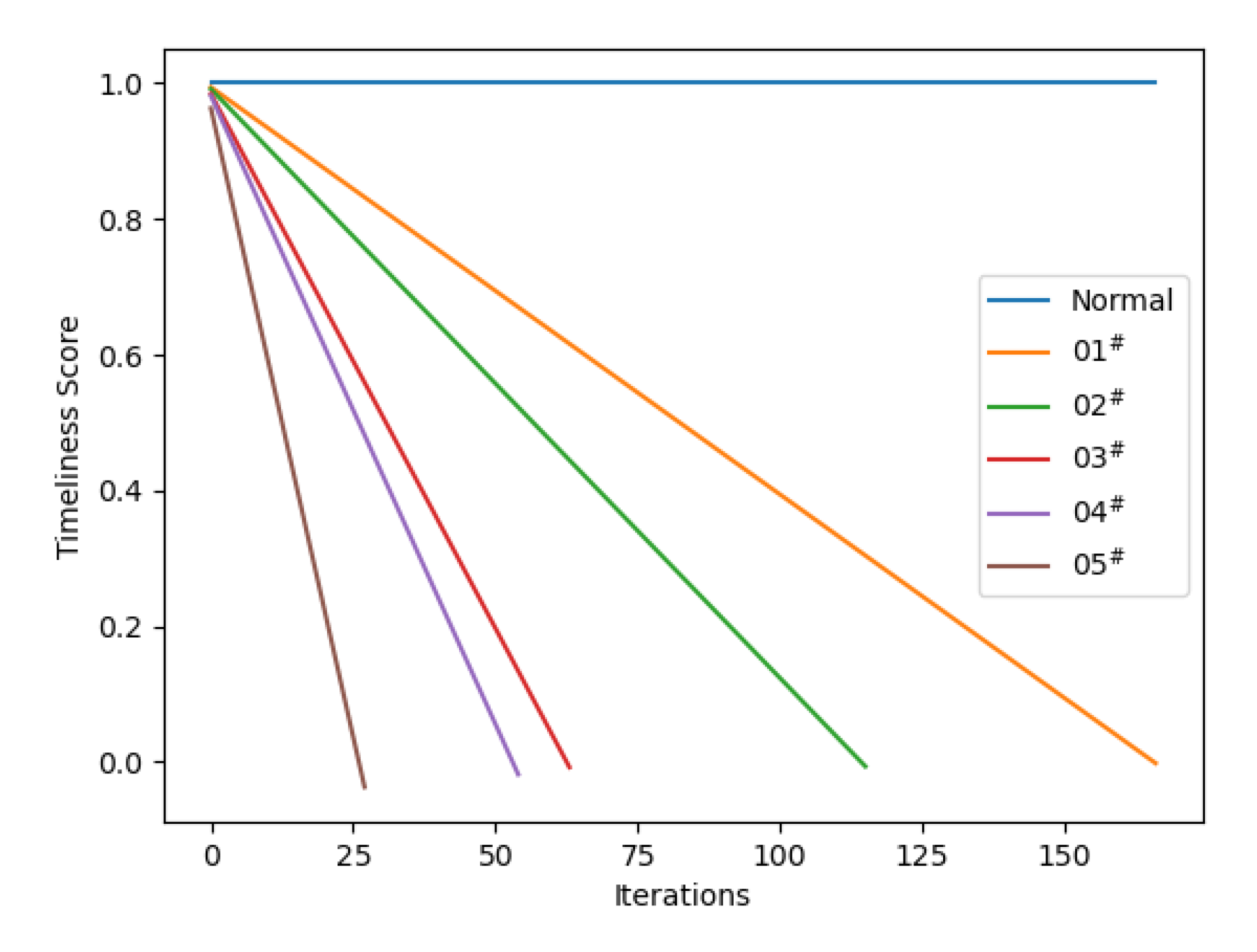
We generated synthetic datasets under different conditions to evaluate the performance of the periodic monitoring model. In order to verify the robustness of the model, we conducted two sets of simulation tests on the synthetic datasets. The first group of tests simulated the number of iterations required for the convergence of our monitoring model when the update time of cycle data in the manufacturing process is always later than the set cycle, as shown in Table 1. The number of iterations required for the convergence of the model when the data update time is always later than the set period ( T = 7 ). Figure 4 shows the trend of the model converging to 0 when the update time is later than the set period to varying degrees. The second group of tests simulated the number of iterations required for the convergence of our monitoring model when the update time of cycle data fluctuates around the set cycle in the manufacturing process, as shown in Table 2. The number of iterations required for the convergence of the model when the data update time is always earlier than the set period ( T = 7 ). Figure 4. Convergence trend of the model when the data are updated later. Figure 5 shows the convergence trend of the model in the case of updating times with different fluctuation amplitudes.
Table 1. The number of iterations required for the convergence of the model when the data update time is always later than the set period ( T = 7 ).
Parameter ValueThe Last
f n t , λ | A  
Iteration Times of
Model Convergence
01 # : α = 0.05, f a l l = 0.2, t = 09−0.002167
02 # : α = 0.05, f a l l = 0.2, t = 11−0.006116
03 # : α = 0.05, f a l l = 0.1, t = 11−0.00864
04 # : α = 0.10, f a l l = 0.1, t = 09−0.01855
05 # : α = 0.20, f a l l = 0.1, t = 09−0.03728
When the data update time is always later than the set period, different parameter configurations correspond to different model convergence speeds, as shown in Table 1. When the update cycle is normalized to T = 7 , we choose to show t = 9 and t = 11 for two main reasons. First, the time series of the input model are normalized to 0 14 , and t = 9 and t = 11 are more representative. Second, because the distribution of the time series is basically in line with the Gaussian distribution through statistical analysis, it is more reasonable to choose two values closer to cycle T = 7 .
Through the comparison of 01 # and 02 # experiments, we found that the same parameter configuration will also have different convergence speeds. The farther away the update time is from the period, the faster the model converges. Through the comparison of experiments 02 # and 03 # , we find that the same update time will also have different convergence speeds. The smaller the decay rate f a l l A , the faster the model converges. Through the comparison of experiments 04 # and 05 # , we find that the larger the periodic update rate α , the faster the model converges. To sum up, the convergence speed of the model is directly proportional to α and inversely proportional to f a l l A . The change trend of the timeliness score of the above five groups of experiments is shown in Figure 4.
Figure 4. Convergence trend of the model when the data are updated later.
Applsci 12 12917 g004
Figure 4 shows that the timeliness score changes linearly with the number of iterations under different parameters. The value of α can be dynamically adjusted according to the sensitivity requirements of different production lines for abnormal monitoring.
The update time of the data is earlier than the set period, and the attenuated value of the data timeliness score should be positive (i.e., Q d e c a y t , λ | A > 0 ) within a period. When the timeliness score after data update is greater than 1, its value will be reset to 1. The number of times greater than 1 is recorded with R A and the value of R A is monitored to reach the set threshold N A (i.e., Formula (10): N A = 100 × f a l l A × 1 α × 1 T t ). Under different parameter configurations, the threshold value to be met for the number of times the evaluation value reaches 1 is shown in Table 2.
Table 2. The number of iterations required for the convergence of the model when the data update time is always earlier than the set period ( T = 7 ).
Parameter ValueSetting of N A
A : α = 0.05, f a l l = 0.2, t = 5200
B : α = 0.05, f a l l = 0.2, t = 3100
C : α = 0.05, f a l l = 0.1, t = 350
D : α = 0.10, f a l l = 0.1, t = 550
E : α = 0.20, f a l l = 0.1, t = 525
Through the comparison between Table 1 and Table 2, it can be seen that under the same parameter configuration, the time to deviate from the set cycle is the same, and the threshold value N A set earlier than the set cycle update has a greater correlation with the number of iterations required to update the model convergence later than the set cycle. For example, the number of iterations (55 times) of the 04 # experiments ( t = 09 ,   t T = 2 ) is close to the threshold N A = 50 set by the parameters of group D ( t = 5 ,   T 3 = 2 ).
In order to test the effectiveness of the model in the case of abnormal fluctuation data (that is, whether the degree of deviation from the set value is the same), the synthetic datasets are input to the model. Table 3 shows the number of iterations required for model convergence under different parameters when the data update time fluctuates before and after the set cycle. Table 3 describes the number of iterations required to change the timeliness score from the initial value of f 1 = 0.5 to f n = 1 or f n = 0 when the data update time fluctuates around the set period. It clearly explains the influence of the time difference between the data update time and the set cycle on the convergence speed of the recurrent timeliness score.
Table 3. The number of iterations required for the convergence of the model when the data update time fluctuates around the set period ( T = 7 ).
Parameter ValueThe Last f n t , λ | A   Iteration Times
06 # : α = 0.05, f a l l = 0.2, t = 6|81.000899
07 # : α = 0.05, f a l l = 0.2, t = 5|91.003227
08 # : α = 0.05, f a l l = 0.1, t = 5|91.001337
09 # : α = 0.05, f a l l = 0.1, t = 6|9−0.001284
10 # : α = 0.05, f a l l = 0.1, t = 5|81.007139
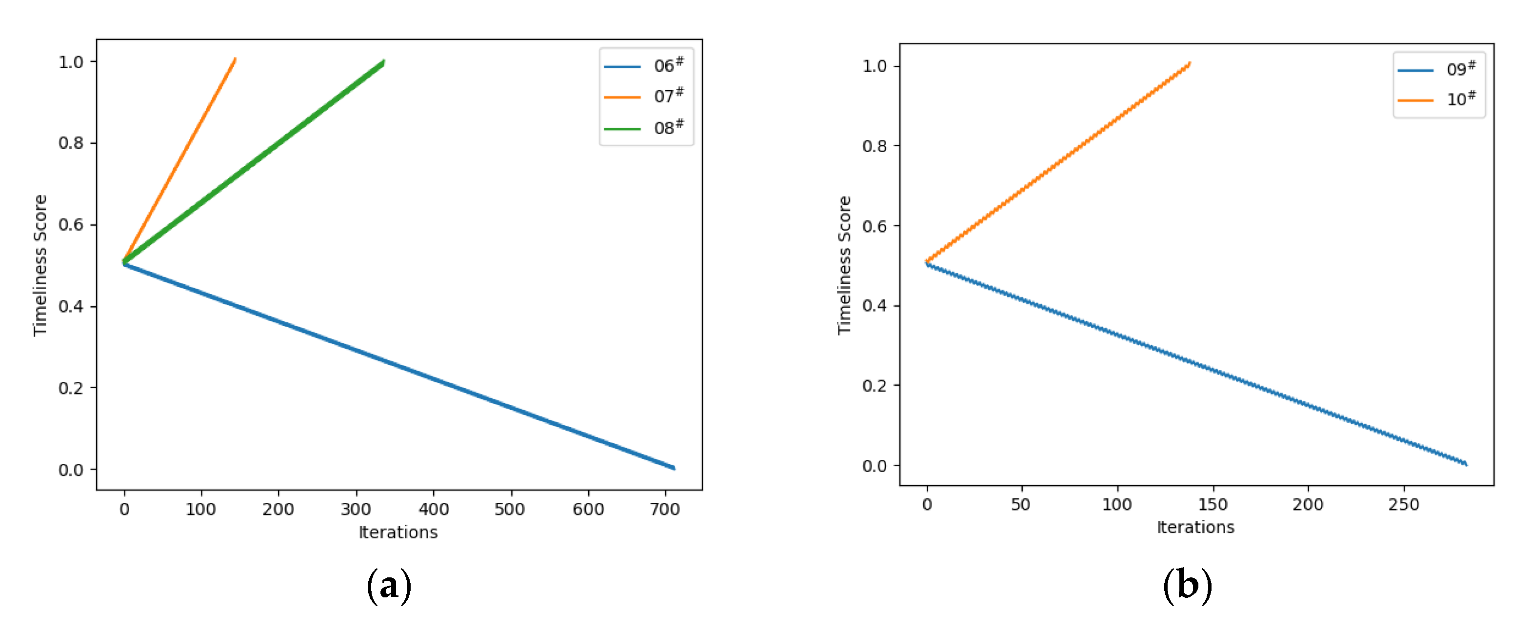
It can be seen from Table 3 that the model can effectively monitor the fluctuating data. Through the statistical analysis of the periodically generated data, it is found that the distribution of the time series basically obeys the Gaussian distribution. According to the data update period of T = 7 and characteristics of Gaussian distribution, t = 6 | 8 and t = 5 | 9 groups of data close to period T = 7 are selected for testing. Through the comparison of 06 # and 07 # , it can be seen that under the same parameter configuration, the greater the fluctuation range, the faster the model converges. Through the comparison of 07 # and 08 # , it can be seen that the smaller the f a l l A value is, the faster the convergence speed of the model is under the same fluctuation amplitude. Abnormal data of symmetric fluctuations were used in the above three groups of experiments. It can be concluded that inputting symmetrical time series to the model will increase or decrease the timeliness score, as shown in Figure 5a. Abnormal data of asymmetric fluctuations were used in the 09 # and 10 # experiments. Through the comparison of 09 # groups and 10 # groups of experiments, two conclusions can be drawn. First, if the time series is later than the cycle, the timeliness score will decrease. Second, if the time series is earlier than the cycle, the timeliness score will rise. The change trend of the experimental timeliness score values of groups 09 # and 10 # with the number of iterations is shown in Figure 5b.
Figure 5. Change trend of score value when periodic data update fluctuates around the set time.
Applsci 12 12917 g005
Figure 5 show that in the case of symmetric data (Figure 5a) and asymmetric data (Figure 5b), respectively, the score of data timeliness changes roughly linearly with the number of iterations. The reason for this change is that the timeliness score decreases exponentially before the arrival of the next updated data. For example, the 09 # experiment always fluctuates around the set period T = 7 , but the deviation degree t = 9 later than the set period is obviously greater than the deviation degree t = 6 earlier than the set period. In this case, the iterative update of the timeliness score tends to zero. This is because when t = 9 , the value of f n + 1 is negative Q 1 , and when t = 6 , the value of f n + 1 is positive Q 2 . At the same time, | Q 1 | is greater than | Q 2 | , so the iterative change of timeliness score tends to zero.

4.2. Conduct Simulation Experiments on Semiconductor Manufacturing Datasets

4.2.1. Experimental Data Set

The data set we use for simulation experiments is Secom. Secom data set first appeared in [27], which is the data collected by various types of sensors in the semiconductor production process. The data set is composed of 591 attributes and signals. A total of 1567 tests (104 of which failed) are recorded, and each test belongs to a production entity. By analyzing the data and finding out the correlation between test failure and test attributes, engineers can first understand the cause of the failure, and then understand which attribute has the greatest impact on the failure. Nearly 7% of the data in Secom data set is lost. These data points have either never been measured, or somehow lost and never entered the final record. However, not all recorded information is useful for data timeliness evaluation. From the perspective of data timeliness evaluation, we only care about the timeseries of Secom dataset. The time series of Secom dataset is shown in Table 4.
Table 4. Datasets of semiconductor manufacturing process.
Serial NumberTime Series
119/07/2008 11:55:00
219/07/2008 12:32:00
319/07/2008 13:17:00
419/07/2008 14:01:00
519/07/2008 14:43:00
155016/10/2008 02:22:00
155116/10/2008 02:55:00
155216/10/2008 03:37:00
155316/10/2008 04:11:00
155416/10/2008 04:58:00
If there are many extreme outlier(s) in the data, the calculated value of A A R D is likely to exceed one [22]. The Secom dataset in this paper has T P = 1463 , F P = 104 , and A A R D = 0.4819 is calculated. It can be seen that the degree of outlier of the dataset is relatively small. It is feasible for this model to use this dataset as an anomaly monitoring simulation experiment.

4.2.2. Process of Simulation Experiment

We have carried out simulation experiments on the data set of the actual semiconductor manufacturing process to test how the model can effectively monitor the abnormalities of the production line. Obviously, the time of data acquisition must be regularized first, especially when the time interval between two data updates is too large. Due to confidentiality, all data labels are anonymous or modified. However, the main results are still valid. As a manufacturing enterprise, the manufacturer is committed to providing users with reliable products. Therefore, the abnormal monitoring ability of the production line plays an important role in the normal work of the manufacturing enterprise.
The RTR model is based on the time stamp of each periodic data update, such as the time series of temperature, humidity, voltage and current generated periodically. The data are generated periodically, and the generated time series are transmitted to the model in real time. Then, the timeliness of periodic data is evaluated based on these time series. On this basis, the evaluation value of data timeliness is monitored for abnormalities. Monitor whether the timeliness score is less than 0 or more than 1 for many times.
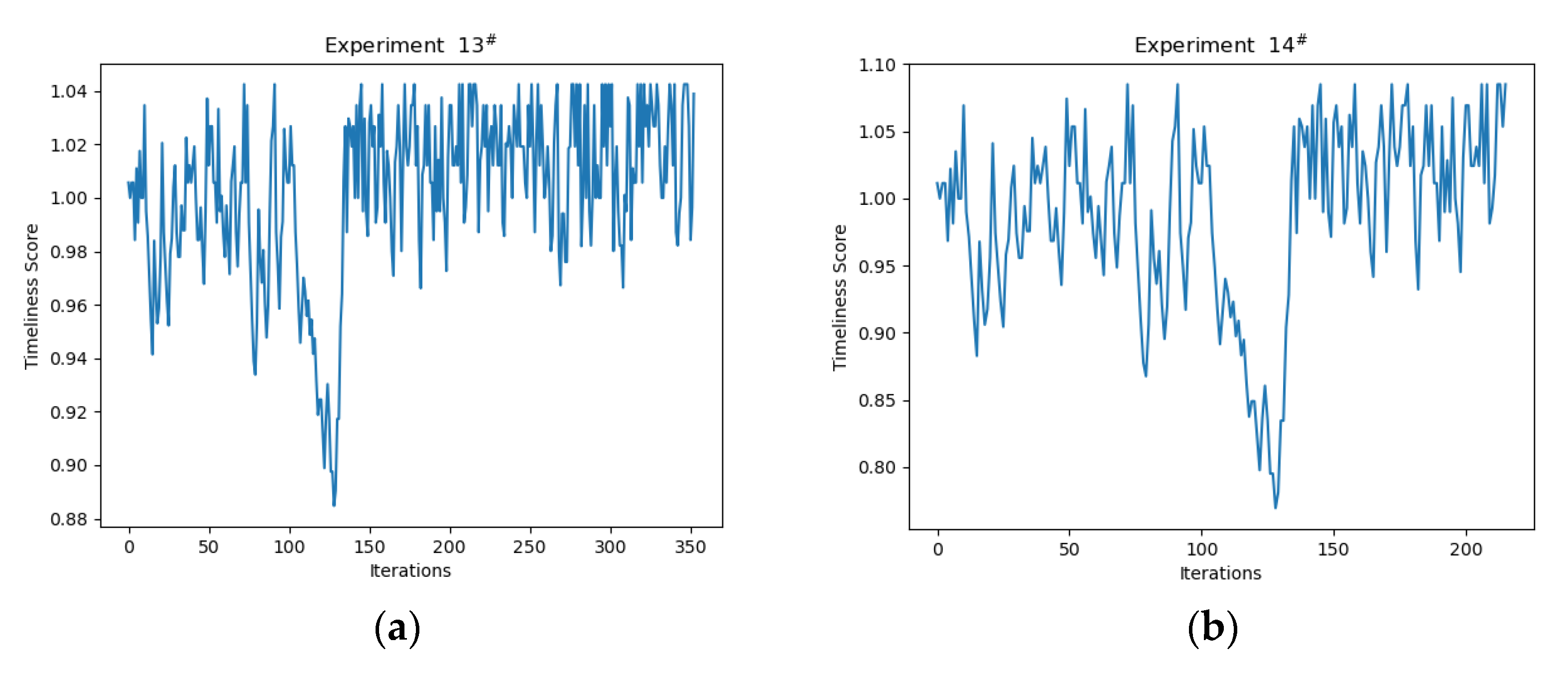
First, we convert all timestamps in the Secom dataset into UNIX timestamps. Then, we calculate the interval of every two adjacent timestamps and normalize the time interval. Finally, we input the processed time series into the RTR model. We conducted four groups of experiments. In these four groups of experiments, f a l l = 0.2 in group 11 # and group 12 # , f a l l = 0.1 in group 13 # and group 14 # . Among them, α = 0.05 in group 11 # and group 13 # experiments, and α = 0.10 in group 12 # and group 14 # experiments. In group 11 # and group 12 # experiments, the condition for model convergence is when the timeliness score is less than 0, as shown in Figure 6. In group 13 # and group 14 # experiments, the condition for model convergence is that the number of times the timeliness score is greater than 1 meets the set threshold, as shown in Figure 7.
Figure 6. The trend of timeliness score converging to 0.
Applsci 12 12917 g006
Figure 6 shows the trend that the timeliness score converges to 0 when two different periodic update rates α are used. Obviously, the larger the periodic update rate α , the faster the model converges.
The timeliness score value of the periodic data at the beginning of the first cycle is set to 1. During the iterative change of the timeliness score of periodic data, we record the times when the timeliness score is greater than 1. Since the maximum timeliness score is 1, it will be reset to 1 when the value is greater than 1. In this case, the condition for model convergence is that the number of times the timeliness score is greater than 1 meets the threshold. According to Formula (10), the threshold value set by group 13 # is 200 ( N A = 100 × f a l l A × 1 α × 1 T t = 100 × 0.1 × 20 × 1 = 200 ), and the threshold value set by group 14 # is 100 ( N A = 100 × f a l l A × 1 α × 1 T t = 100 × 0.1 × 10 × 1 = 100 ). Figure 7 shows the change of timeliness score.
Figure 7. The fluctuation amplitude of timeliness score is different under the two parameters.
Applsci 12 12917 g007
From Figure 7, we can conclude that the smaller the value of α , the faster the model converges. In addition, the larger the value of α , the larger the change range of the timeliness score. For example, when the f a l l value is the same and the 13 # experiment α = 0.05 is less than the 14 # experiment α = 0.1 , the number of iterations of the experiment shown in Figure 7a (up to 350) is greater than the number of iterations of the experiment shown in Figure 7b (more than 200). At the same time, we can see that the fluctuation range of timeliness score in Figure 7a (about 0.93 1.04 ) is smaller than that in Figure 7b (about 0.85 1.10 ).
In order to test the operation effect of the model considering multiple attributes (such as temperature, humidity, pressure, flow, etc.), we divided the original data set into four. According to Formulas (8) and (9), we carried out simulation experiments 15 # . The experimental 15 # results are shown in Figure 8.
Figure 8. The convergence trend of the model considering multiple attributes.
Applsci 12 12917 g008
In Figure 8, we consider four attributes: temperature, humidity, pressure and flow. Finally, the model converges because the timeliness score of the humidity attribute reaches 0. We can choose the appropriate α value according to the requirements of different properties of products on the sensitivity of abnormal monitoring, so that the production process can be dynamically adjusted.

4.3. Summary of the Experiment

Since the AMP-RTR model needs to process each generated data in turn, the time complexity of the model is 0 n . In addition, the spatial complexity of the model is mainly divided into two parts: one is to store the timeliness score value after each iteration update, and the spatial complexity of this part is 0 n ; the other part uses R A to record the times greater than the set threshold N A , and the spatial complexity of this part is 0 1 , so the spatial complexity of this model should be 0 n + 0 1 = 0 n , where n represents the size of the data volume.
In summary, we tested the robustness of the AMP-RTR model by performing 10 sets of simulation experiments on a synthetic dataset; we then performed four sets of simulation experiments on the semiconductor dataset to verify the applicability of the AMP-RTR model; finally, we performed a set 15 simulation experiments by splitting the original semiconductor dataset into four, validating the performance of the AMP-RTR model when accounting for multivariate properties.

5. Conclusions

In this paper, based on the theory of time stamp based timeliness evaluation method, and in view of the characteristics of periodic data generation, the Recurrent Timeliness Rules (RTR) is proposed. These rules define the basis for the regularity change of periodic data timeliness; that is, the attenuation function of the timeliness evaluation value in the data update cycle and Iteration principle of timeliness evaluation value. According to RTR, the updating iteration method of timeliness evaluation value is proposed. Therefore, the Anomaly Monitoring of Process based on Recurrent Timeliness Rules (AMP-RTR) is constructed. The AMP-RTR model monitors the regularity change of periodic data timeliness to measure the possibility of abnormality in the production line. The AMP-RTR model monitors the regularity change for periodic data timeliness by adjusting the decay rate f a l l A and periodic update rate α , so as to meet the customized requirements for monitoring sensitivity of different production lines in the manufacturing industry.
The robustness test of the AMP-RTR model with synthetic dataset shows that the model can monitor the abnormal situation of data bias and fluctuation. The applicability test of the AMP-RTR model with the semiconductor data set shows that the model can monitor anomalies according to the regularity change for periodic data timeliness. The semiconductor data set is divided into four parts, and the test results of temperature, humidity, flow rate and pressure on the AMP-RTR model show that the actual production line has good performance in anomaly monitoring. The analysis of the above 15 groups of simulation experiments shows that AMP-RTR model has strong applicability. The A A R D method is used to measure the experimental data set used by the model, A A R D = 0.4819 . It can be seen that the degree of outlier of the data set is relatively small, indicating that the simulation experiment of the AMP-RTR model is effective.
It is a complex and arduous task to evaluate the timeliness of periodic data and monitor the abnormal production process. In future research, the following two attempts can be made. First, in the timeliness evaluation of periodic data, because the equipment, process and environment involved in different industrial production lines are quite different, we can try to summarize the timeliness attenuation function corresponding to different scenarios. Second, we can try to set the threshold value N A as a dynamic change value, evaluate the timeliness of data, and monitor the abnormalities in the production process.

Author Contributions

Conceptualization, Y.J.; methodology, Z.L. and X.D.; validation, X.D. and J.T.; formal analysis, D.H. and J.T.; writing—original draft preparation, Z.L.; writing—review and editing, Z.L.; supervision, D.H. and Y.J. All authors have read and agreed to the published version of the manuscript.

Funding

This work was supported in part by the National Key R&D Program of China under Grant No. 2020YFB1707900 and 2020YFB1711800; the National Natural Science Foundation of China under Grant No. 62262074 U2268204 and 62172061; the Science and Technology Project of Sichuan Province under Grant No. 2022YFG0159, 2022YFG0155, 2022YFG0157, 2021GFW019, 2021YFG0152, 2021YFG0025 and 2020YFG0322.

Institutional Review Board Statement

Not applicable.

Informed Consent Statement

Not applicable.

Data Availability Statement

Not applicable.

Acknowledgments

It is our pleasure to acknowledge Ke Du and Chao Tang for their assistance and support with this project.

Conflicts of Interest

The authors declare no conflict of interest.

References

  1. Li, M.; Li, J.; Cheng, S.; Sun, Y. Uncertain Rule Based Method for Determining Data Currency. IEICE Trans. Inf. Syst. 2018, E101.D, 2447–2457. [Google Scholar] [CrossRef] [Green Version]
  2. Batini, C.; Scannapieco, M. Data and Information Quality: Dimensions, Principles and Techniques; Springer: Berlin/Heidelberg, Germany, 2016. [Google Scholar]
  3. Kaiser, M.; Klier, M.; Heinrich, B. How to Measure Data Quality? A Metric-Based Approach. ICIS 2007 2007, 31, 108. [Google Scholar]
  4. Even, A.; Shankaranarayanan, G.; Berger, P.D. Evaluating a Model for Cost-effective Data Quality Management in A Real-world CRM Setting. Decis. Support Syst. 2010, 50, 152–163. [Google Scholar] [CrossRef]
  5. Firmani, D.; Mecella, M.; Scannapieco, M.; Batini, C. On the Meaningfulness of “Big Data Quality” (Invited Paper). Data Sci. Eng. 2015, 1, 6–20. [Google Scholar] [CrossRef] [Green Version]
  6. Hevner, A.R.; March, S.T.; Park, J.; Ram, S. Design Science in Information Systems Research. Manag. Inf. Syst. Q. 2004, 28, 75. [Google Scholar] [CrossRef] [Green Version]
  7. Ballou, D.; Wang, R.; Pazer, H.; Tayi, G.K. Modeling Information Manufacturing Systems to Determine Information Product Quality. Manag. Sci. 1998, 44, 462–484. [Google Scholar] [CrossRef] [Green Version]
  8. Even, A.; Shankaranarayanan, G. Utility-driven Assessment of Data Quality. ACM SIGMIS Database: Database Adv. Inf. Syst. 2007, 38, 75–93. [Google Scholar] [CrossRef]
  9. Li, F.; Nastic, S.; Dustdar, S. Data Quality Observation in Pervasive Environments. In Proceedings of the 2012 IEEE 15th International Conference on Computational Science and Engineering, Paphos, Cyprus, 5–7 December 2012; pp. 602–609. [Google Scholar]
  10. Heinrich, B.; Klier, M. Metric-based data quality assessment—Developing and Evaluating a Probability-based Currency Metric. Decis. Support Syst. 2015, 72, 82–96. [Google Scholar] [CrossRef]
  11. Dalip, D.H.; Goncalves, M.A.; Cristo, M.; Calado, P. Automatic Quality Assessment of Content Created Collaboratively by Web Communities: A Case Study of Wikipedia. In Proceedings of the 9th Annual International ACM/IEEE Joint Conference on Digital Libraries, Austin, TX, USA, 15–19 June 2009; pp. 295–304. [Google Scholar]
  12. Dalip, D.H.; Lima, H.; Goncalves, M.A.; Cristo, M.; Calado, P. Quality Assessment of Collaborative Content with Minimal Information. In Proceedings of the 14th IEEE/ACM Joint Conference on Digital Libraries (JCDL)/18th International Conference on Theory and Practice of Digital Libraries (TPDL), London, UK, 8–12 September 2014; pp. 201–210. [Google Scholar]
  13. Warncke-Wang, M.; Cosley, D.; Riedl, J. Tell me more: An Actionable Quality Model for Wikipedia. In Proceedings of the 9th International Symposium on Open Collaboration, Hong Kong, China, 5–7 August 2013; Association for Computing Machinery: New York, NY, USA, 2013. Article 8. [Google Scholar]
  14. Dang, Q.V.; Ignat, C.L. Measuring Quality of Collaboratively Edited Documents: The case of Wikipedia. In Proceedings of the 2nd IEEE International Conference on Collaboration and Internet Computing (IEEE CIC), Pittsburgh, PA, USA, 1–3 November 2016; pp. 266–275. [Google Scholar]
  15. Dang, Q.-V.; Ignat, C.-L. An End-to-end Learning Solution for Assessing the Quality of Wikipedia Articles. In Proceedings of the 13th International Symposium on Open Collaboration, Galway, Ireland, 23–25 August 2017; Association for Computing Machinery: New York, NY, USA, 2017. Article 4. [Google Scholar]
  16. Heinrich, B.; Klier, M. A Novel Data Quality Metric for Timeliness Considering Supplemental Data. In 17th European Conference on Information Systems (ECIS); University of Verona: Verona, Italy, 2009. [Google Scholar]
  17. Azeroual, O.; Saake, G.; Wastl, J. Data Measurement in Research Information Systems: Metrics for The Evaluation of Data Quality. Scientometrics 2018, 115, 1271–1290. [Google Scholar] [CrossRef]
  18. Heinrich, B.; Klier, M.; Kaiser, M. A Procedure to Develop Metrics for Currency and its Application in CRM. J. Data Inf. Qual. 2009, 1, 1–28. [Google Scholar] [CrossRef] [Green Version]
  19. Klier, M.; Moestue, L.; Obermeier, A.A.; Widmann, T. Event-Driven Assessment of Currency of Wiki Articles: A Novel Probability-Based Metric. ICIS 2021 Proc. 2021, 14. Available online: https://aisel.aisnet.org/icis2021/data_analytics/data_analytics/14 (accessed on 10 October 2022).
  20. Ibrahimi, K.; Cherif, O.O.; Elkoutbi, M.; Rouam, I. Model to Improve the Forecast of the Content Caching based Time-Series Analysis at the Small Base Station. In Proceedings of the 2019 International Conference on Wireless Networks and Mobile Communications (WINCOM), Fez, Morocco, 29 October–1 November 2019; pp. 1–6. [Google Scholar]
  21. Torres Labrada, R. Multi-signal Anomaly Detection for Real-Time Embedded Systems. Master’s Thesis, University of Waterloo, Waterloo, ON, Canada, 2020. [Google Scholar]
  22. Prusty, B.R.; Jain, N.; Ranjan, K.G.; Bingi, K.; Jena, D. New Performance Evaluation Metrics for Outlier Detection and Correction. In Sustainable Energy and Technological Advancements; Advances in Sustainability Science and Technology; Springer: Singapore, 2022; pp. 837–845. [Google Scholar]
  23. Batini, C.; Cappiello, C.; Francalanci, C.; Maurino, A.; Viscusi, G. A capacity and Value Based Model for Data Architectures Adopting Integration Technologies. In Proceedings of the 17th Americas Conference on Information Systems, AMCIS 2011, Detroit, MI, USA, 4–8 August 2011. [Google Scholar]
  24. Pipino, L.L.; Lee, Y.W.; Wang, R.Y. Data Quality Assessment. Commun. ACM 2002, 45, 211–218. [Google Scholar] [CrossRef]
  25. Heinrich, B.; Klier, M. Assessing data currency—A Probabilistic Approach. J. Inf. Sci. 2011, 37, 86–100. [Google Scholar] [CrossRef] [Green Version]
  26. Cho, J.; Garcia-Molina, H. Effective Page Refresh Policies for Web Crawlers. ACM Trans. Database Syst. 2003, 28, 390–426. [Google Scholar] [CrossRef]
  27. McCann, M.; Li, Y.; Maguire, L.; Johnston, A. Causality Challenge: Benchmarking Relevant Signal Components for Effective Monitoring and Process Control. J. Mach. Learn. Res. 2010, 6, 277–288. [Google Scholar]
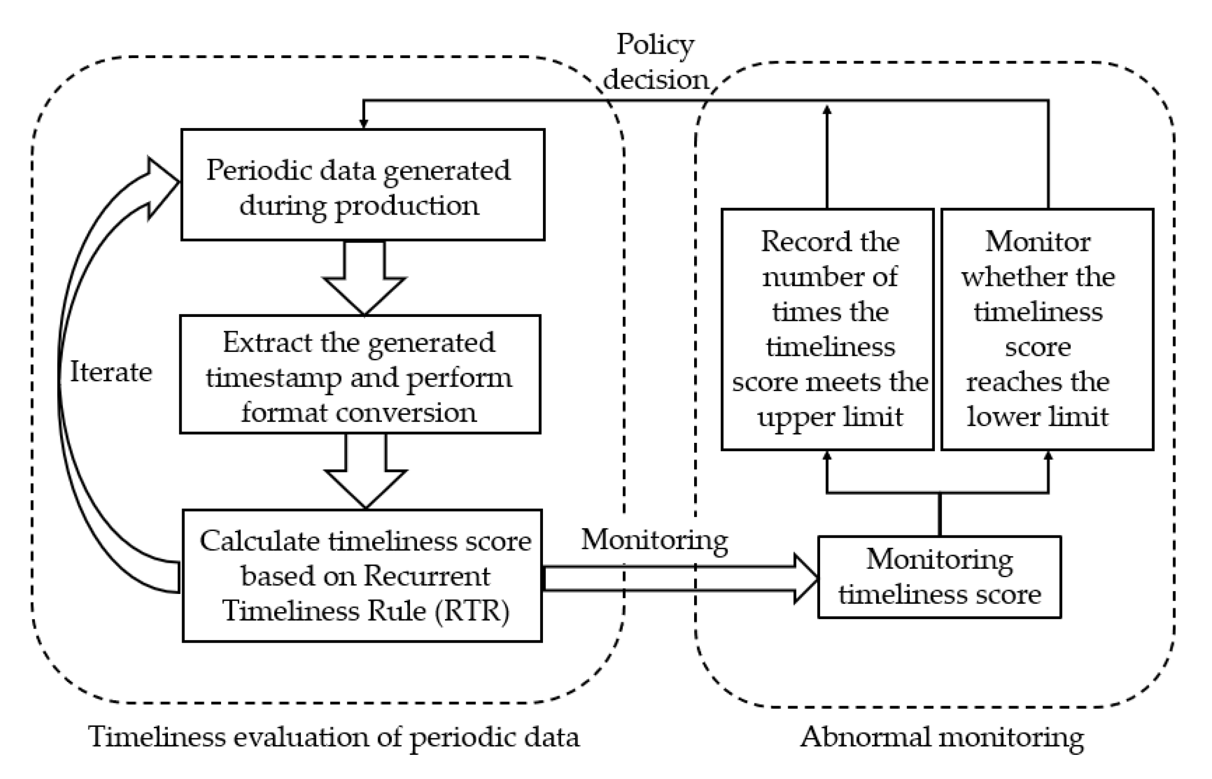
Figure 1. The AMP-RTR research flow diagram.
Applsci 12 12917 g001
Figure 3. Flow chart of abnormal monitoring.
Applsci 12 12917 g003
Publisher’s Note: MDPI stays neutral with regard to jurisdictional claims in published maps and institutional affiliations.