An Enhanced Water Quality Index for Water Quality Monitoring Using Remote Sensing and Machine Learning

Abstract

Water quality deterioration is a serious problem with the increase in the urbanization rate. However, water quality monitoring uses grab sampling of physico-chemical parameters and a water quality index method to assess water quality. Both processes are lengthy and expensive. These traditional indices are biased towards the physico-chemical parameters because samples are only collected from certain sampling points. These limitations make the current water quality index method unsuitable for any water body in the world. Thus, we develop an enhanced water quality index method based on a semi-supervised machine learning technique to determine water quality. This method follows five steps: (i) parameter selection, (ii) sub-index calculation, (iii) weight assignment, (iv) aggregation of sub-indices and (v) classification. Physico-chemical, air, meteorological and hydrological, topographical parameters are acquired for the stream network of the Rawal watershed. Min-max normalization is used to obtain sub-indices, and weights are assigned with tree-based techniques, i.e., LightGBM, Random Forest, CatBoost, AdaBoost and XGBoost. As a result, the proposed technique removes the uncertainties in the traditional indexing with a 100% classification rate, removing the necessity of including all parameters for classification. Electric conductivity, secchi disk depth, dissolved oxygen, lithology and geology are amongst the high weighting parameters of using LightGBM and CatBoost with 99.1% and 99.3% accuracy, respectively. In fact, seasonal variations are observed for the classified stream network with a shift from 55:45% (January) to 10:90% (December) ratio for the medium to bad class. This verifies the validity of the proposed method that will contribute to water management planning globally.

1. Introduction

Water is an essential resource for the sustenance of all living organisms. Being a significant resource, its quality needs to be monitored and managed properly. However, it is constantly being affected by anthropogenic activities caused by growing urbanization. Factors such as soil erosion and climate change can have a huge impact on the physical landscape of water bodies. These factors are usually ignored while assessing water quality, and traditionally, only the physico-chemical parameters, such as turbidity, conductivity and pH are used. However, such factors are not enough to accurately analyse the conditions that can have an impact on the water body. Thus, topographical and hydrological parameters, such as slope, aspect, lithology, geology and soil type, may have a direct/indirect impact on the overall quality of the water body. Similarly, the abundance of air pollutants such as nitrogen and carbon dioxide can cause water eutrophication [1], acidification [2] and nutrient pollution [3] that can be harmful for the aquatic ecosystem. Moreover, heavy precipitation can also directly affect the water cycle resulting in the deterioration of the water bodies [4].

In reality, the monitoring of multiple contamination sources is a tedious and expensive task that involves field visits and laboratory work. Utilizing remote sensing and machine learning technology to overcome such challenges is being used by many researchers [5]. This, in turn, can make the sampling process more robust and economical. In fact, such technology can be utilized to assess water quality based on the combined impact of different parameters that can be a complex task otherwise. Traditionally, a water quality index (WQI) is a weighted average of selected ambient concentrations of pollutants providing a single number that represents the overall water quality at a certain location and time. The most frequently used WQIs include the National Sanitation Foundation Water Quality Index (NSFWQI) [6], the Canadian Council of Ministers of the Environment Water Quality Index (CCME) [7], the Oregon Water Quality Index (OWQI) [8], etc. However, the application of the WQIs on water samples is a biased approach as each index is built specific to certain locations or water types or is sensitive to specific parameter concentrations or dependency on the weights assigned [9]. Such limitations make the traditional WQIs unsuitable for application on any general water body.

To overcome these challenges, an enhanced water quality index (EWQI) is proposed in this research that uses machine learning and data mining methods to analyse the combined impact of different factors, including hydrological, topographical, meteorological, air and physico-chemical parameters and assigns appropriate weights using the tree-based, i.e., CatBoost and LightGBM, methods. Thus, a machine learning approach is proposed as a replacement WQI that can remove the bias and can be applied to any water body regardless of the selected parameters. A total of twenty-two parameters are extracted for the time period of July 2018 to August 2022 that include seven water quality parameters, i.e., total dissolved solids (TDS), pH, electrical conductivity (EC), Secchi disk depth (SDD), dissolved oxygen (DO), turbidity (Tur) and chlorophyll-$\alpha$ (chl-$\alpha$) are acquired from the Sentinel-2 Multispectral Imager (S2-MSI) Level 1C (L1C) satellite; six air pollutants that include carbon monoxide (CO), nitrogen dioxide ($N{O}_2$), ozone ($O_3$), sulphur dioxide ($S{O}_2$), formaldehyde (HCHO) and methane ($C{H}_4$) are acquired from the Sentinel-5 Precursor Level 2 (S5P-L2) TROPOspHeric Monitoring Instrument (TROPOMI); three meteorological parameters, namely air temperature, wind speed and total precipitation are taken from the ERA5 Climate Reanalysis Project, (ERA5-CRP); and lastly, six hydrological and topographical parameters that include slope, aspect, soil type, lithology, geology and land use/land cover are acquired from the Digital Elevation Model (DEM) created with Shuttle Radar Topography Mission (SRTM) data. The NSFWQI method that uses the water quality parameters for evaluation is used to compare the quality of the Rawal Stream Network with the new proposed EWQI that is based on the extracted twenty-two parameters. Moreover, using a remote sensing and machine learning approach can help in analyzing the different factors affecting water quality which are applicable on a global scale. This research reveals that the new proposed EWQI is a much more reliable and accurate index compared to the state-of-the-art NSFWQI method as it: (i) operates well with or without missing parameters, (ii) identifies the temporal and seasonal variations, and (iii) considers all other environmental factors while classifying the water body. The major contributions of this study are as follows:

• Twenty-two parameters are extracted for the stream network of the Rawal watershed that include seven water quality parameters, six air pollutants and three meteorological and six hydrological/topographical parameters pertaining to the years (2018–2022) for the monsoon months of June to September.
• A multimodal indexing technique, EWQI, is proposed that involves five steps: parameter selection, sub-index calculation, weight assignment, aggregation of sub-indices and classification using a machine learning approach for weight assignment, sub-index calculation and remote sensing technology for parameter selection to extract twenty-two multimodal parameters.

This paper is organized as follows: Section 2 discusses the related work. Section 3 explains the proposed EWQI. Section 4 covers the proposed methodology for the extraction of the twenty-two parameters, and the application of the EWQI method is discussed for the Rawal stream network. The results of the comparison between NSFWQI and EWQI are discussed in Section 5. In Section 6, the conclusion of this research is presented.

2. Literature Review

WQIs that are based on physico-chemical and biological parameters are used for monitoring the quality of water at different locations, such as the United Kingdom [10], Dalmatia [11], Zimbabwe [12], Argentina [13] and India [14]. Over the years, a number of water quality indices have been proposed that first convert raw parameter concentrations into a sub-index or quality rating (q) value and aggregate these indices to obtain a final water quality index value [15]. This value lies in the range of 0 to 100 and is classified accordingly [16]. Among the most commonly used WQIs are NSFWQI, CCME, OWQI, weighted arithmetic WQI (WAWQI) and minimum operator index (MOI) [17]. The classification and number of parameters used for these indices are given in Table 1. WAWQI and NSFWQI use the unit weight (w) and q of the nth parameter to calculate the final WQI value as seen in Table 1. The CCME is based on: (1) scope $F_1$, (2) frequency $F_2$ and (3) amplitude $F_3$.

Table 1. Classification of WQI values for five Indices.

Index	No. of Parameters	WQI Value	Rating Class	Equation	Reference
WAWQI	10			$WAWQI=\frac{{\sum }_{i=1}^n{q}_i{w}_i}{{\sum }_{i=1}^n{w}_i}$	[18]
		0 to 25	Excellent	n = the number of parameters,
		25 to 50	Good	$q_n$ = quality rating of the nth parameter,
		51 to 75	Fair	$w_n$ = unit weight of the nth parameter
		76 to 100	Poor
		101 to 150	Very Poor
		Above 150	Unfit for Drinking
NSFWQI	9			$NSFWQI={\sum }_{i=1}^n{w}_i{q}_i$	[6]
		90 to 100	Excellent	n = the number of parameters,
		70 to 90	Good	$q_n$ = quality rating of the nth parameter,
		50 to 70	Medium	$w_n$ = unit weight of the nth parameter
		25 to 50	Bad
		0 to 25	Very Bad
CCME	47			$CCME=100-\left[\begin{array}{c}\frac{\sqrt{F_1^2+F_2^2+F_3^2}}{1.732}\end{array}\right]$	[7]
		95.0 to 100.0	Excellent	$F_1$ = No. of Failed/ Total variables × 100
		80.0 to 94.9	Good	$F_2$ = No. of Failed/ Total tests × 100
		65.0 to 79.9	Fair	$F_3$ = amount by which objectives not met
		45.0 to 64.9	Marginal
		0.0 to 44.9	Poor
OWQI	8			OWQI = $\sqrt{\frac{n}{{\sum }_{i=1}^n\frac{1}{S{I}_i^2}}}$	[8]
		to 100	Excellent	n = number of parameters,
		85 to 89	Good	$S{I}_i$ = SI is the sub-index for the ith parameter
		80 to 84	Fair
		60 to 79	Poor
		less than 60	Very Poor
MOI	8			MOI = $min(S{I}_1,S{I}_2,\cdots ,S{I}_n)$	[17]
		80 to 100	Eminently suitable for all uses	n = number of parameters,
		60 to 79	Suitable for all uses	$S{I}_n$ = SI is the sub-index for the nth parameter
		40 to 59	Main use may be compromised
		20 to 39	Unsuitable for several uses
		0 to 19	Totally unsuitable for many uses

Some of these indices use expert opinions in identifying important parameters, weight assignment and transformation to sub-indices [10]. Other development techniques include fuzzy interference [19] and the Delphi method is used in NSFWQI, OWQI and the index of water quality (IWQ) [20]. However, the common attribute amongst these indices is the use of physico-chemical variables. Of parameters used, 6% are biological, 24% are physical, and 70% are chemical [21]. Amongst them, the DO, total coliforms have an 87% selection rate [22]. Biological oxygen demand and pH are selected at a 73% rate [23]. Temperature, Tur, ammonia and TDS have a 47% selection rate [24]. The problem identified for most of these indices is that they are very sensitive to the parameters involved in classifying a water body. Even a single parameter with a slightly high concentration value can affect the index classification [9]. Studies have used grab sampling or data acquisition from government authorities to analyze physico-chemical parameters such as pH [25], conductivity [26], hardness [27], and phosphate [28], and the WQI is calculated to identify the underlying issues.

The literature reveals that the traditional indices are based on specific physico-chemical water parameters and thus have limitations that make these indices unsuitable for worldwide use. The uncertainty of the WQIs makes them unpredictable for complex environmental situations [29]. These indices are biased to a set of parameters, place, area and purpose of use. The dynamic nature of the water body can cause certain changes in the physico-chemical properties [30]. Moreover, the influence of air pollutants, meteorological features and hydrological features on the aquatic ecosystems is ignored in the development of the WQI method [31]. These challenges indicate that most WQIs fail to accurately classify a water body. Therefore, there is a need for a universally accepted index that removes the uncertainties and bias in the traditional standards.

3. Enhanced Water Quality Index

The WQI development method involves five common steps [32] that include parameter selection, sub-index calculation, weight assignment, sub-indices aggregation and classification. To enhance the methodology involved in the development of this technique, machine learning methods are used. Moreover, instead of using the traditional water quality standards for weight assignment, a tree-based scoring technique is used. For the development of the EWQI, the methods are trained on the training set, and the best performing technique is applied on the test set. The process is further described in detail as follows:

3.1. Parameter Selection

Most WQI development techniques involve subjective methods for selection of parameters that include water regulatory organizations, the Delphi method and expert opinion. Multiple parameters are involved in the calculation of a single WQI value. These mostly include the physico-chemical characteristics of the water bodies. Generally, these parameters are not enough for assessing the water quality of any water body. Certain parameters, such as hydrological, air and meteorological variables, can influence water quality in a wider manner and cannot be neglected in the calculation of the WQI value.

3.2. Sub-Index Calculation

This step is used to transform the different parameters to a uniform scale. Each parameter has a different unit. For example, the physico-chemical parameters, i.e., DO and chl-$\alpha$, are measured in mg/L. Air pollutants are measured in mol/m² for $N{O}_2$, $S{O}_2$, CO, $O_3$, $HCHO$ and parts per million (ppm) for $C{H}_4$. The meteorological parameters are measured in ms⁻¹ for wind speed and Kelvin for air temperature. Similarly, slope is given in % and aspect parameter in degrees. Traditionally, the transformation of parameters is performed by linear, non-linear functions, fuzzy membership and expert opinion that may involve using national and international standards. These standards are applied to a formula to obtain a sub-index value in the range of 100. In machine learning, the normalization of parameters is a common data preprocessing step. The most used normalization is the min–max method. Here, this technique is applied to the preprocessed training data to transform the values in a 0–100 range. The new sub-index formula is given in Equation (1), where q = sub-index value, v = parameter value, $ma{x}_A$ = maximum value of the parameter, and $mi{n}_A$ = minimum value of the parameter.

$$q=\frac{v-mi{n}_A}{ma{x}_A-mi{n}_A}(100-0)$$

(1)

3.3. Weight Assignment

This step involves assigning weights to each parameter. Previously, WQI calculation involved assigning unequal weights to parameters [6] or giving equal weights or no weights [7]. Usually, this is accomplished by assigning a 1–5 range to the variables. The high priority variables are given a weighting of five and low priority variables a value of one. Then, relative weights are computed. This method is known as the ranking method. Other weighting techniques are expert opinion, fuzzy interference and the Delphi method. Such weighting methods can introduce bias in the method and are dependent on the inclusion of all the selected parameters. Any missing parameter will directly affect the resultant WQI value. In our index, this process is replaced by a semi-supervised technique that involves first clustering the data and then applying an algorithm. The K-means clustering method is applied on the training data. The Elbow method is used to obtain the number of K. Once the training set is clustered, the tree-based feature importance scores are calculated. There are five tree-based feature importance methods in machine learning, i.e., XGBoost (XGB), Random Forest (RF), LightGBM (LGBM), CatBoost (CatB) and AdaBoost (AdaB) are taken to obtain weights for the parameters, and then the relative weights are computed. The final weights with the highest accuracy are used to calculate the EWQI on the test set. Equation (2) shows the formula for the relative weight of the parameter n where $S_n$ = Score of the nth parameter.

$$W_n=\frac{S_n}{{\sum }_{i=1}^n{S}_i}$$

(2)

3.4. Sub-Indices Aggregation

Once the weights are assigned and the sub-index values are calculated, the EWQI is computed by aggregating the values using either geometric or arithmetic mean, logarithmic function or root square. The formula for the EWQI is given in Equation (3). Here, n is the number of the parameters selected which are mentioned in Section 3.1, $q_n$ is the quality rating or sub-index of the nth parameter which is calculated by Equation (1), and $W_n$ is the relative weight of the nth parameter calculated by Equation (2).

$$EWQI=\frac{{\sum }_{i=1}^n{q}_i{W}_i}{{\sum }_{i=1}^n{W}_i}$$

(3)

3.5. Classification

The values of the computed EWQI are classified in five categories: (i) excellent (90–100), (ii) good (70–90), (iii) medium (50–70), (iv) bad (25–50), and (v) poor (<25).

4. Methodology

The methodology for the application of the EWQI is given in detail in this section. The proposed EWQI is applied on the study area of the Rawal watershed. Figure 1 shows the high-level methodology applied for the acquisition of features and development of the new index.

Figure 1. The steps involved in the extraction of multimodal parameters (1–7), extraction of samples (8), dataset formation (9), calculation and application of the EWQI for the study area (10,11).

4.1. Study Area

The Rawal watershed [33] begins at a lake located at latitude: 33${}^{\circ }$42${}^{\prime }$ N, longitude: 73${}^{\circ }$7${}^{\prime }$ E in Islamabad, Pakistan which supplies water to a population of around 3 million. Using Geographic Information System (GIS) tools, a water stream network is extracted from the Rawal watershed to analyze the water-associated properties of the area, excluding the land attributes. The SRTM [34] data is mosaicked for the selected region to create a DEM, and sequentially, a stream network is clipped by applying the GIS hydrology tools. Figure 2 shows the DEM of the study area, i.e., the Rawal watershed encompassing the stream network.

Figure 2. Study area map for the Rawal watershed located in Islamabad, Pakistan.

4.2. Data Acquisition

Four categories of data are acquired which encompass (i) aysicochemical parameters, (ii) hydrological and topographical parameters, (iii) air parameters, and (iv) meteorological parameters. The sources of the extracted parameters are listed in Table 2.

Table 2. Types of data acquired and their sources.

Category	Type of Data	Sources
Physicochemical Parameters	TDS pH EC SDD DO Tur chl-$\alpha$	SRTM DEM S2-MSI L1C [35]
Hydrological and Topographical Parameters	Slope Aspect	SRTM DEM
	Soil Type	SRTM DEM Digital Soil Map [36]
	Geology Lithology	SRTM DEM GeoTypes [37]
	Land use/Land Cover	SRTM DEM ESA Worldcover [38]
Air Parameters	CO	SRTM DEM Earth Engine [39]
	$N{O}_2$	SRTM DEM S5P-L2 TROPOMI Earth Engine [40]
	$O_3$	SRTM DEM S5P-L2 TROPOMI Earth Engine [41]
	$S{O}_2$	SRTM DEM S5P-L2 TROPOMI Earth Engine [42]
	HCHO	SRTM DEM S5P-L2 TROPOMI Earth Engine [43]
	$C{H}_4$	SRTM DEM S5P-L2 TROPOMI Earth Engine [44]
Meteorological Parameters	Air Temperature Wind Speed Total Precipitation	SRTM DEM ERA5-CRP Earth Engine [45]

4.2.1. Physico-Chemical Parameters

The data was acquired from the Google Earth Engine, which comprised S2-MSI L1C images for extracting water quality parameters. The SRTM data is used for the creation of DEM. The S2-MSI L1C contains Top of Atmosphere (TOA) images factored by a value of 10,000. These images were observed for the monsoon season, i.e., June to September of 2018 to 2022 for the Rawal stream network. The different band compositions of the images were used to acquire physical parameters for the stream network using the adapted equations for calculating the TDS, pH, EC, SDD, DO, Tur and chl-$\alpha$ that are mentioned in Table 3. The equation (given in Table 3) shows the Tur and chl-$\alpha$ calculation, which are based on bands 3, 4 and 8a that gave a Root Mean Square Error (RMSE) of 7.65 NTU and 10.15 mg/L, respectively, when observed with the ground truth values obtained for the study area. The equation for pH shows an RMSE of 3.36 using bands 11, 3 and 4. EC is based on band 11 with an RMSE of 228.7 mS/cm. DO and TDS are based on bands 8a and 1 with an RMSE of 2.82 mg/L and 111.92 mg/L, respectively. Lastly, bands 2 and 4 are used to calculate SDD with an RMSE of 0.22 m. Figure 3 shows a sample of the parameters extracted for July 2020.

Table 3. Adapted equations for water quality parameters.

Parameter	Adapted Equations	Reference	RMSE
Tur	35.121 − 14.489 ((R3)/(R4)) − 0.911 (R8a)	[46]	7.65 NTU
pH	8.790 + 0.141 (R11) − 0.228 (R3/R4)	[47]	3.36
EC	422.034 − 1080.365 (R11)	[47]	228.7 mS/cm
chl-$\alpha$	54.658 + 520.451 (R2) − 1221.89 (R3) + 611.115 (R4) − 198.199 (R8a)	[48]	10.15 mg/L
DO	10.841 − 0.682 ((R1)/(R8a)) − 0.002 ((R2)/(R8a) + (B2))	[47]	2.82 mg/L
TDS	120.750 + 264.752 (R8a/R1)	[47]	111.92 mg/L
SDD	0.2 + 1.4 ln (R2/R4)	[49]	0.22 m

Figure 3. Physicochemical parameters for the Rawal watershed.

4.2.2. Hydrological and Topographical Parameters

The hydrological and topographical parameters were acquired from the different sources that are mentioned in Table 2. The slope for the study area was then acquired from the DEM using ArcGIS tools. The slope attribute extracted for the observed study area is classified into six classes; (i) flat (0–3%), (ii) gentle sloping (3–8%), (iii) sloping (8–15%), (iv) moderately steep (15–30%), (v) steep (30–50%), and (vi) very steep (>50%) as seen in Figure 4. The Rawal watershed mostly lies in the moderately steep class. The steepness of the slopes determines the momentum of the runoff. Faster run off can cause soil erosion that naturally ends up in the waterways, causing the water to pollute. Thus, the moderately steep slope with a partial runoff is considered to have a good water quality. Similarly, the aspect parameter was derived from the DEM and distributed in 10 classes namely; (i) flat (−1), (ii) north (0–22.5), (iii) northeast (22.5–67.5), (iv) east (67.5–112.5), (v) southeast (112.5–157.5), (vi) south (157.5–202.5), (vii) southwest (202.5–247.5), (viii) west (247.5–292.5), (ix) northwest (292.5–337.5), and (x) north (337.5–360) as seen in Figure 4. The impact of sun is determined by the aspect parameter which gives an understanding of the plants that colonize the slope and eventually determines the animals that may be seeking food. The Rawal watershed has a south-facing slope which is warmer, and the soil tends to dry out faster in such slopes. The soil type parameter is also an important attribute that plays a part in assessing the quality of the water. Soils with higher infiltration capacity can decrease the runoff to a great degree. The soil types for the Rawal watershed are classified as (i) Be—eutric cambisois and (ii) Rc—calcaric regosois, with a 99:1% ratio. The eutric cambisois class lies in the hydro group B category which means that such soil types have a moderate infiltration rate.

Figure 4. Hydrological and Topographical Parameters for the Rawal watershed.

Moreover, the topographical parameters, i.e., the geological formations, of the study area are classified as Cenozoic and Upper Paleozoic (Dev, Car, Per) with a 44:56% ratio. Lithology for the Rawal watershed has siliciclastic sedimentary consolidated (Ss) and mixed sedimentary consolidated (Sm) rocks with a 44:56% ratio. Such rocks have a high resistance to erosion and poor solubility rate. Additionally, the type of land use is an important factor in determining the behaviour of the watershed as they affect the water infiltration rate. The land use/land cover parameter for the watershed is classified as (i) trees, (ii) shrubland, (iii) grassland, (iv) cropland, (v) built-up, (vi) barren/sparse vegetation, (vii) open water, and (viii) herbaceous wetland.

4.2.3. Air Parameters

The air parameters were extracted from S5P-L2 satellite images that comprise six pollutants: CO, $N{O}_2$, $O_3$, $S{O}_2$, HCHO and $C{H}_4$, shown in Figure 5. The $N{O}_2$ concentrations are extracted using band 4 of the TROPOMI L2’s UV, UV-VIS spectrometer [50]. Band 3 of the UV-VIS spectrometer is used to derive the $HCHO$ [51], $O_3$ [52] and $S{O}_2$ [53] concentrations. Band 7 of the SWIR spectrometer is used to measure $C{H}_4$ and $CO$ concentrations [54].

Figure 5. Air parameters for the Rawal watershed.

4.2.4. Meteorological Parameters

Air temperature, wind speed and total precipitation were extracted from the ERA5-CRP [55], shown in Figure 6. This project has a climate data store that was assembled using assimilation and advanced modelling to obtain the historical observations into a global consistent form. The air temperature is at a 2 m distance, and wind speed is at a 10 m distance from the surface of the Earth.

Figure 6. Meteorological parameters for the Rawal watershed.

4.3. Data Preprocessing

Data were acquired using the Google Earth Engine [56] software. The maps were prepared by Arc-Map 10.8 [57]. The S2-MSI L1C, S5P-L2, ERA5-CRP images were preprocessed to extract the parameters from the selected Rawal watershed DEM. GIS clipping tools were used to select the target boundaries from the image to extract the area of interest. A total of 4998 points were extracted from each monsoon month in the time period of July 2018 to August 2022, giving a total of 284,889 or approximately 0.3 M sample points. These sample points were extracted from the Rawal stream network as the watershed region covers a land and water region. To make a dataset with all the features, the four categories of data were joined based on the matching dates and latitude–longitude. The hydrological and topographical data is consistent or stable data that generally remains the same regardless of the time and is joined on the basis of matching latitude–longitude. Once the sample points are extracted and the dataset with the twenty-two parameters is created, a set of preprocessing techniques is performed that include:

• Replacing the missing values: The missing values are replaced using imputation techniques. The numerical data is imputed with the average or mean. The categorical data is imputed using the most frequent value method.
• Replacing the categorical data: The categorical data is converted to numeric form by using the encoding technique. For example, geology (Cenozoic: 1, Upper Paleozoic (Dev, Car, Per): 2), soil type (Be: 1, Rc: 2), lithology (Ss: 1, Sm: 2) and land cover/land use (trees: 10, shrubland: 20, grassland: 30, cropland: 40, built-up: 50, barren/sparse vegetation: 60, snow and ice: 70, open water: 80, herbaceous wetland: 90).
• Splitting the dataset: The data are split into train and test sets with a 60:40 ratio.

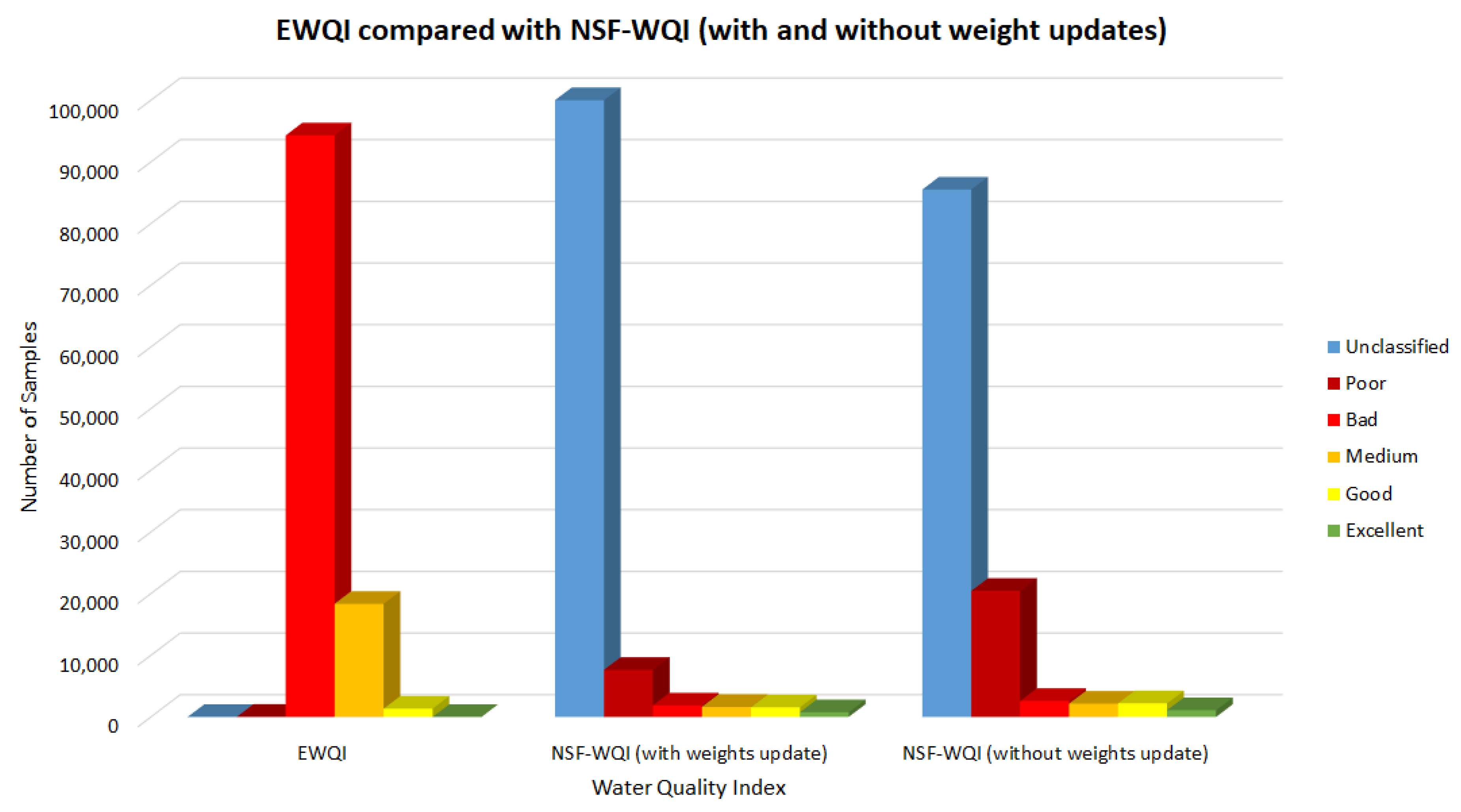
5. Results and Discussion

Once the dataset is compiled and preprocessed using the methods mentioned in Section 4, the selected twenty-two parameters are used for calculating the EWQI. These include six air pollutants (CO, $N{O}_2$, $O_3$, $S{O}_2$, HCHO and $C{H}_4$), six hydrological parameters (lithology, land use/land cover, soil type, slope, aspect and geology), three meteorological variables (air temperature, wind speed and total precipitation) and seven physico-chemical water quality features (TDS, pH, EC, SDD, DO, Tur and chl-$\alpha$). The selection of parameters is reassessed in the “Weight Assignment” stage using the tree-based algorithms. Next, the selected parameters are transformed using min–max normalization to a range of 0–100. The physico-chemical parameters, i.e., DO and chl-$\alpha$ are measured in mg/L, while air pollutants are measured in mol/m². Thus, this step is necessary to obtain a uniform dataset.

Then, a feature weighting technique is applied. For this step, the dataset is divided into 60:40% train and test sets. Both the training and test set results are mentioned. Moreover, with the 40% test set used to verify the proposed technique, a set of test data is acquired for the year 2020. This test set is taken to explore the EWQI results whether the index is functional under seasonal restrictions or there are certain missing parameters such as the state-of-the-art NSF method. It contains the days from other seasons besides the monsoon months that were originally used in the training dataset. This will help in the analysis and verification of the newly developed EWQI. The optimal number of clusters is four for the preprocessed train data. The clustering is performed to categorize the data samples as Class 1, 2, 3 and 4. Once the data is clustered and labelled, tree-based feature weighting is applied to obtain the parameter scores.

Table 4 shows the weighting methods, scores and accuracy achieved on the training data. The best accuracy of 99.34% and 99.1% was achieved with the CatB and LGBM methods. The LGBM gave the best accuracy with 21 parameters, where the “Geology” parameter is discarded. The CatB method gave its best accuracy with the 22 parameters. Table 4 also shows the parameter scores of the feature weighting methods. XGB gave the highest scores to EC, SDD and lithology parameters. RF gave the highest scores to EC, TDS and geology, whereas LGBM gave SDD, pH, DO and O₃ the highest scores. Geology, EC, lithology and DO are the top scorers for CatB. This proves that multiple parameters play a part in categorizing the water. In order to test this hypothesis, the weighting methods were also tested for physico-chemical parameters alone and physico-chemical, air and meteorological parameters. Table 5 shows the results for the selected parameters for the top performing algorithms where the highest accuracy achieved was up to 82%. The dependencies of different parameters on the water quality can be seen with the inclusion of all 22 parameters that gave a 99% accuracy rate.

Table 4. Feature weighting method results on the training data.

Feature Weighting Method	No. of Parameters	Score		Accuracy
XGB	20	chl-$\alpha$: 0.00183 DO: 0.07315 EC: 0.19124 pH: 0.04043 SDD: 0.12290 TDS: 0.08795 Tur: 0.00593 Air Temperature: 0.00382 Precipitation: 0.02134 Wind: 0.01571 CO: 0.00534	$N{O}_2$: 0.03497 $O_3$: 0.02866 $S{O}_2$: 0.00398 HCHO: 0.01529 $C{H}_4$: 0.00246 Aspect: 0.00316 Slope: 0.00147 Lithology: 0.33722 Landcover: 0.00314	98.46%
RF	22	chl-$\alpha$: 0.04159 DO: 0.08917 EC: 0.13447 pH: 0.09033 SDD: 0.06160 TDS: 0.11201 Tur: 0.04504 Air Temperature: 0.00448 Precipitation: 0.00896 Wind: 0.00844 CO: 0.01142	$N{O}_2$: 0.02785 $O_3$: 0.03457 $S{O}_2$: 0.00452 HCHO: 0.01582 $C{H}_4$: 0.00056 Aspect: 0.00520 Slope: 0.00955 Lithology: 0.14103 Soil Type: 0.00087 Landcover: 0.01397 Geology: 0.13857	98.83%
LGBM	21	chl-$\alpha$: 269.00000 DO: 1092.00000 EC: 790.00000 pH: 1181.00000 SDD: 1287.00000 TDS: 777.00000 Tur: 221.00000 Air Temperature: 337.00000 S9: 325.00000 Wind: 325.00000 CO: 676.00000	$N{O}_2$: 790.00000 $O_3$: 1072.00000 $S{O}_2$: 287.00000 HCHO: 735.00000 $C{H}_4$: 98.00000 Aspect: 390.00000 Slope: 489.00000 Lithology: 482.00000 Soil Type: 9.00000 Landcover: 368.00000	99.11% 2
CatB	22	chl-$\alpha$: 1.96433 DO: 10.02918 EC: 12.98044 pH: 6.98978 SDD: 6.19110 TDS: 5.29395 Tur: 3.04026 Air Temperature: 1.40388 Precipitation: 1.21085 Wind: 1.76956 CO: 2.32570	$N{O}_2$: 3.83250 $O_3$: 5.40983 $S{O}_2$: 1.50510 HCHO: 3.38323 $C{H}_4$: 0.13716 Aspect: 1.13175 Slope: 1.91270 Lithology: 11.99015 Soil Type:0.10634 Landcover: 1.96139 Geology: 15.43083	99.34% 1
AdaB	16	DO: 0.08000 EC: 0.10000 pH: 0.08000 SDD: 0.10000 TDS: 0.12000 Precipitation: 0.04000 Wind: 0.02000 CO: 0.04000	$N{O}_2$: 0.04000 $O_3$: 0.06000 $S{O}_2$: 0.06000 HCHO: 0.02000 Slope: 0.10000 Lithology: 0.02000  Landcover: 0.04000 Geology: 0.08000	85.49%

¹ The first highest accuracy achieved ² The second highest accuracy achieved.

Table 5. Feature weighting method results on the training data for selected parameters.

Feature Weighting Method	No. of Parameters	Score		Accuracy
CatB	7	chl-$\alpha$: 8.99274, DO: 24.24110, EC: 22.92371, pH: 10.68041, SDD: 12.36481, TDS: 13.93459, Tur: 6.86264		78%
LGBM	16	chl-$\alpha$: 604.00000 DO: 1325.00000 EC: 993.00000 pH: 1468.00000 SDD: 1212.00000 TDS: 1131.00000 Tur: 494.00000 Air Temperature: 311.00000	Precipitation: 298.00000 Wind Speed: 301.00000 CO: 718.00000 $N{O}_2$: 973.00000 $O_3$: 1021.00000 $S{O}_2$: 311.00000 HCHO: 785.00000 $C{H}_4$: 55.00000	81.88%

The results of the classification achieved with the top two performing feature weighting techniques on the test set are given in Table 6. CatB weights classified the test set in four classes, i.e., bad (82.7%), medium (16%), poor (1.2%) and good (0.005%), whereas the LGBM classified the test data in two classes, i.e., bad (82.6%) and medium (17%). The test data was also classified using the traditional NSFWQI method. The weights in the NSFWQI were assigned based on the selection of the physico-chemical parameters. Thus, the NSFWQI weights need to readjusted for the current physico-chemical parameters used. The results of the classification of the test set using EWQI (CatB weighting), NSFWQI (without weight updates) and NSFWQI (with weight updates) is shown in Figure 7. Figure 7 represents the classification of samples with EWQI, NSFWQI (with weights updated) and NSFWQI (without weights updated). It shows the number of samples that fall in each class i.e., poor, bad, medium and excellent. It can be seen that with NSFWQI, more than 75% of the data remains unclassified, even with weight updates. This, in turn, proves that the results achieved with the EWQI are reliable and accurate.

Table 6. Relative weights and the classified samples using CatB and LGBM methods on the test set.

Method	Relative Weights (${\mathit{W}}_{\mathit{n}}$)		Class	No. of Samples
CatB	$W_1$ = 0.019643 $W_2$ = 0.100292 $W_3$ = 0.129804	$W_{11}$ = 0.023257 $W_{12}$ = 0.038325 $W_{13}$ = 0.054098	Bad	94,282
	$W_4$ = 0.069898 $W_5$ = 0.061911 $W_6$ = 0.052939 $W_7$ = 0.030403	$W_{14}$ = 0.015051 $W_{15}$ = 0.033832 $W_{16}$ = 0.001372 $W_{17}$ = 0.011317	Medium	18,336
	$W_8$ = 0.014039 $W_9$ = 0.012108	$W_{18}$ = 0.019127 $W_{19}$ = 0.119901 $W_{20}$ = 0.001063	Good	1332
	$W_{10}$ = 0.017696	$W_{21}$ = 0.019614 $W_{22}$ = 0.154308	Poor	6
LGBM	$W_1$ = 0.022417 $W_2$ = 0.091 $W_3$ = 0.065833 $W_4$ = 0.098417 $W_5$ = 0.10725	$W_{11}$ = 0.056333 $W_{12}$ = 0.065833 $W_{13}$ = 0.089333 $W_{14}$ = 0.023917 $W_{15}$ = 0.06125	Bad	94,103
	$W_6$ = 0.06475 $W_7$ = 0.018417 $W_8$ = 0.028083 $W_9$ = 0.027083 $W_{10}$ = 0.027083	$W_{16}$ = 0.008167 $W_{17}$ = 0.0325 $W_{18}$ = 0.04075 $W_{19}$ = 0.040167 $W_{20}$ = 0.00075 $W_{21}$ = 0.030667 $W_{22}$ = 0	Medium	19,853

Figure 7. EWQI compared with NSF-WQI (with and without weight updates) on the test data.

Figure 8 and Figure 9 show the map for the classified Rawal stream network using both EWQI and NSFWQI. Test samples for 3 September 2018 and 2019 are classified as bad (shown in red) and medium (shown in orange) classes with EWQI, whereas the samples are mostly unclassified with the NSFWQI method.

Figure 8. EWQI compared with NSFWQI for 3 September 2018 (test data).

Figure 9. EWQI compared with NSFWQI for 3 September 2019 (test data).

In addition to the 40% test data that are acquired for the monsoon months (June–September), 4998 sample points are collected from each non-monsoon or winter season of the year 2020. These data are used to further analyze the performance of the EWQI and are compared with the traditional NSFWQI. Table 7 shows the results for the test sets of six months, i.e., January, February, March, April, November and December 2020. The NSFWQI failed to classify the test subsets for these months of 2020. The parameters used for NSFWQI are the seven physico-chemical water quality parameters. The test sets for the year 2020 had some missing parameters, such as for November and December the meteorological parameters are missing, for January 2020 $C{H}_4$ is missing. However, even with the missing parameters, the EWQI weights are applicable and have classified the data which is in contrast to the application of NSFWQI. Moreover, it can be seen that with EWQI throughout January to March, the classified samples have a 55:45 ratio for medium to bad class. However, for April this ratio shifted to 90:10. For November, the ratio further shifted to 45:55 and finally for December, the ratio wass 10:90. The 10% to 90% ratio of medium to bad class indicates the river water pollution that occurs due to anthroprogenic activities during winter [58]. This shows that the seasonal variations are visible with the EWQI method that is trained on the data collected for just monsoon months. Figure 10 and Figure 11 display the test samples for January and February using the EWQI (LGBM) method. These classification maps are produced in ArcMap after applying post classification smoothing [59] using spatial analyst tools.

Table 7. Results on test subsets acquired for non-monsoon months of the year 2020.

Test Set	Parameters	Method	Class	Samples
26 January 2020	21	EWQI (LGBM)	Medium	2856
			Bad	2137
			Good	4
	7	NSFWQI	Unclassified	4998
10 February 2020	21	EWQI (LGBM)	Medium	2537
			Bad	2461
	7	NSFWQI	Unclassified	4998
1 March 2020	22	EWQI (LGBM)	Medium	2551
			Bad	2447
	7	NSFWQI	Unclassified	4998
10 April 2020	21	EWQI (LGBM)	Medium	4081
			Bad	917
	7	NSFWQI	Unclassified	4998
26 November 2020	17	EWQI (LGBM)	Medium	2030
			Bad	2968
	7	NSFWQI	Unclassified	4998
6 December 2020	16	EWQI (LGBM)	Medium	846
			Bad	4152
	7	NSFWQI	Unclassified	4998

Figure 10. EWQI for 26 January 2020 (test data).

Figure 11. EWQI for 10 February 2020 (test data).

Although EWQI has all six levels of water quality like the NSFWQI method, the Rawal stream network does not contain samples that fall in all six classes as seen with the acquired data. Thus, this is a limitation of the study, and in future, other lakes and watersheds can be investigated with the EWQI to show samples that belong to all the classes.

6. Conclusions

The physico-chemical, hydrological and topographical air pollutants and meteorological parameters were extracted from S2-MSI L1C, SRTM DEM, S5P-L2 and ERA5-CRP, respectively, for the Rawal stream network for the monsoon months (June to September) for the years 2018 to 2022. The water quality was assessed using WQI methodology to rank the water bodies. However, the application of the WQIs on water samples is a biased approach as each index is built specific to certain locations or water types or is sensitive to specific parameter concentrations or is dependent on the weights assigned. Such limitations make the traditional WQIs unsuitable for application on any general water body. Thus, this study aimed to determine the impact of other natural factors in the environment to understand and classify the water quality using an enhanced water quality index method. An enhanced indexing methodology is proposed that, compared to the traditional or state-of-the-art WQI, is based on a multitude of parameters and machine learning techniques. The first step of building the EWQI method was the parameter selection, where 22 physico-chemical, hydrological and topographical air pollutants and meteorological parameters were selected, i.e., lithology, geology, soil type, wind speed, air temperature, CO, $N{O}_2$, $O_3$, DO, TDS, etc. Next, the sub-index calculation was performed using the min–max normalization technique to transform the data in the 0 to 100 range. The third and most crucial step was assigning weights where the train data was clustered using the Elbow method to find the K value. The final weights were then calculated on the clustered train data with LGBM and CatB models giving a 99% accuracy. These weights were then assigned to the test data. Once the sub-index and weights were calculated, the sub-indices aggregation took place by applying the formula given in Equation (3). The final step was the classification of the EWQI values using the WHO ranking system.

The conclusions drawn from the analysis of the newly proposed indexing technique are that the use of tree-based LGBM weighting and min–max normalization methods can lead to the accurate classification of the stream network as compared to the traditional NSFWQI. Moreover, the parameters, i.e., physico-chemical and other natural factors such as air pollutants, air temperature, slope, aspect, etc. all play a role in categorizing the water quality where EC, SDD, DO, lithology and geology are given high scores or weights with the feature weighting methods LGBM and CatB. Contrary to the NSFWQI, the missing parameters do not influence the classification of the water body using the EWQI. Even with more than five missing parameters for November and December 2020, the classification maps are produced with each sample assigned to a bad, medium or good class. The EWQI works well for all seasons as the seasonal variations can also be observed for January to December where the water quality class ratio shifted from 55:45 to 10:90 ratio for medium to bad class. In contrast, NSFWQI failed to classify the samples. Thus, the new and improved EWQI method will help remove the uncertainties involved in the traditional methods and can contribute to water management planning on a global scale. In the future, the EWQI can be explored further for other water bodies such as Khanpur, Mangla and Tarbela Dam.

References

- Yang, X.E.; Wu, X.; Hao, H.L.; He, Z.L. Mechanisms and assessment of water eutrophication. J. Zhejiang Univ. Sci. B 2008, 9, 197–209. [Google Scholar] [CrossRef]
- Doney, S.C.; Fabry, V.J.; Feely, R.A.; Kleypas, J.A. Ocean acidification: The other CO2 problem. Annu. Rev. Mar. Sci. 2009, 1, 169–192. [Google Scholar] [CrossRef]
- Board, O.S.; National Research Council. Clean Coastal Waters: Understanding and Reducing the Effects of Nutrient Pollution; National Academies Press: Washington, DC, USA, 2000. [Google Scholar]
- Puczko, K.; Jekatierynczuk-Rudczyk, E. Extreme hydro-meteorological events influence to water quality of small rivers in urban area: A case study in Northeast Poland. Sci. Rep. 2020, 10, 1–14. [Google Scholar] [CrossRef] [PubMed]
- Yang, X.; Zheng, Y.; Geng, G.; Liu, H.; Man, H.; Lv, Z.; He, K.; de Hoogh, K. Development of PM2.5 and NO2 models in a LUR framework incorporating satellite remote sensing and air quality model data in Pearl River Delta region, China. Environ. Pollut. 2017, 226, 143–153. [Google Scholar] [CrossRef] [PubMed]
- McClelland, N.I. Water Quality Index Application in the Kansas River Basin; US Environmental Protection Agency: Washington, DC, USA, 1974; Volume 74.
- Canadian Council of Ministers of the Environment. Canadian Water Quality Guidelines for the Protection of Aquatic Life: CCME Water Quality Index 1.0, User’s Manual; Canadian Council of Ministers of the Environment: Winnipeg, MB, Canada, 2001. [Google Scholar]
- Cude, C.G. Oregon water quality index a tool for evaluating water quality management effectiveness 1. J. Am. Water Resour. Assoc. 2001, 37, 125–137. [Google Scholar] [CrossRef]
- Ahmed, M.; Mumtaz, R.; Hassan Zaidi, S.M. Analysis of water quality indices and machine learning techniques for rating water pollution: A case study of Rawal Dam, Pakistan. Water Supply 2021, 21, 3225–3250. [Google Scholar] [CrossRef]
- House, M.; Newsome, D. Water quality indices for the management of surface water quality. In Urban Discharges and Receiving Water Quality Impacts; Elsevier: Amsterdam, The Netherlands, 1989; pp. 159–173. [Google Scholar]
- Nives, S.G. Water quality evaluation by index in Dalmatia. Water Res. 1999, 33, 3423–3440. [Google Scholar]
- Jonnalagadda, S.; Mhere, G. Water quality of the Odzi River in the eastern highlands of Zimbabwe. Water Res. 2001, 35, 2371–2376. [Google Scholar] [CrossRef]
- Pesce, S.F.; Wunderlin, D.A. Use of water quality indices to verify the impact of Córdoba City (Argentina) on Suquía, River. Water Res. 2000, 34, 2915–2926. [Google Scholar] [CrossRef]
- Sargaonkar, A.; Deshpande, V. Development of an overall index of pollution for surface water based on a general classification scheme in Indian context. Environ. Monit. Assess. 2003, 89, 43–67. [Google Scholar] [CrossRef]
- Ott, W.R. Environmental Indices: Theory and Practice. 1978. Available online: https://www.osti.gov/biblio/6681348 (accessed on 3 September 2022).
- Bouza-Deaño, R.; Ternero-Rodríguez, M.; Fernández-Espinosa, A. Trend study and assessment of surface water quality in the Ebro River (Spain). J. Hydrol. 2008, 361, 227–239. [Google Scholar] [CrossRef]
- Smith, D.G. A better water quality indexing system for rivers and streams. Water Res. 1990, 24, 1237–1244. [Google Scholar] [CrossRef]
- Brown, R.M.; McClelland, N.I.; Deininger, R.A.; O’Connor, M.F. A water quality index—Crashing the psychological barrier. In Indicators of Environmental Quality; Springer: Berlin/Heidelberg, Germany, 1972; pp. 173–182. [Google Scholar]
- Lermontov, A.; Yokoyama, L.; Lermontov, M.; Machado, M.A.S. River quality analysis using fuzzy water quality index: Ribeira do Iguape river watershed, Brazil. Ecol. Indic. 2009, 9, 1188–1197. [Google Scholar] [CrossRef]
- Dinius, S. Design of An Index of Water Quality. J. Am. Water Resour. Assoc. 1987, 23, 833–843. [Google Scholar] [CrossRef]
- Soumaila, K.I.; Niandou, A.S.; Naimi, M.; Mohamed, C.; Schimmel, K.; Luster-Teasley, S.; Sheick, N.N. A systematic review and meta-analysis of water quality indices. J. Agric. Sci. Technol. B 2019, 9, 1–14. [Google Scholar]
- Said, A.; Stevens, D.K.; Sehlke, G. An innovative index for evaluating water quality in streams. Environ. Manag. 2004, 34, 406–414. [Google Scholar] [CrossRef]
- Liou, S.M.; Lo, S.L.; Wang, S.H. A generalized water quality index for Taiwan. Environ. Monit. Assess. 2004, 96, 35–52. [Google Scholar] [CrossRef]
- Gitau, M.W.; Chen, J.; Ma, Z. Water quality indices as tools for decision making and management. Water Resour. Manag. 2016, 30, 2591–2610. [Google Scholar] [CrossRef]
- Srebotnjak, T.; Carr, G.; de Sherbinin, A.; Rickwood, C. A global Water Quality Index and hot-deck imputation of missing data. Ecol. Indic. 2012, 17, 108–119. [Google Scholar] [CrossRef]
- Selvam, S.; Manimaran, G.; Sivasubramanian, P.; Balasubramanian, N.; Seshunarayana, T. GIS-based evaluation of water quality index of groundwater resources around Tuticorin coastal city, South India. Environ. Earth Sci. 2014, 71, 2847–2867. [Google Scholar] [CrossRef]
- Wu, Z.; Wang, X.; Chen, Y.; Cai, Y.; Deng, J. Assessing river water quality using water quality index in Lake Taihu Basin, China. Sci. Total. Environ. 2018, 612, 914–922. [Google Scholar] [CrossRef] [PubMed]
- Karunanidhi, D.; Aravinthasamy, P.; Subramani, T.; Muthusankar, G. Revealing drinking water quality issues and possible health risks based on water quality index (WQI) method in the Shanmuganadhi River basin of South India. Environ. Geochem. Health 2021, 43, 931–948. [Google Scholar] [CrossRef] [PubMed]
- Silvert, W. Fuzzy indices of environmental conditions. Ecol. Model. 2000, 130, 111–119. [Google Scholar] [CrossRef]
- Khan, F.I.; Abbasi, S. Multivariate hazard identification and ranking system. Process. Saf. Prog. 1998, 17, 157–170. [Google Scholar] [CrossRef]
- Ahmed, M.; Mumtaz, R.; Baig, S.; Zaidi, S.M.H. Assessment of correlation amongst physico-chemical, topographical, geological, lithological and soil type parameters for measuring water quality of Rawal watershed using remote sensing. Water Supply 2022, 22, 3645–3660. [Google Scholar] [CrossRef]
- Swamee, P.K.; Tyagi, A. Improved method for aggregation of water quality subindices. J. Environ. Eng. 2007, 133, 220–225. [Google Scholar] [CrossRef]
- Ali, M.; Qamar, A.M.; Ali, B. Data analysis, discharge classifications, and predictions of hydrological parameters for the management of Rawal Dam in Pakistan. In Proceedings of the 2013 12th International Conference on Machine Learning and Applications, Miami, FL, USA, 4–7 December 2013; Volume 1, pp. 382–385. [Google Scholar]
- Van Zyl, J.J. The Shuttle Radar Topography Mission (SRTM): A breakthrough in remote sensing of topography. Acta Astronaut. 2001, 48, 559–565. [Google Scholar] [CrossRef]
- Sentinel-2 MSI: Multispectral Instrument, Level-1c|Earth Engine Data Catalog|Google Developers. Available online: https://developers.google.com/earth-engine/datasets/catalog/COPERNICUS_S2 (accessed on 26 October 2022).
- Digital Soil Map. Available online: https://worldmap.harvard.edu/data/geonode:DSMW_RdY (accessed on 26 October 2022).
- GeoTypes. Available online: http://geotypes.net/downloads.html (accessed on 26 October 2022).
- Esa Worldcover 10 m V100|Earth Engine Data Catalog|Google Developers. Available online: https://developers.google.com/earth-engine/datasets/catalog/ESA_WorldCover_v100 (accessed on 26 October 2022).
- Sentinel-5P OFFL CO: Offline Carbon Monoxide|Earth Engine Data Catalog|Google Developers. Available online: https://developers.google.com/earth-engine/datasets/catalog/COPERNICUS_S5P_OFFL_L3_CO (accessed on 26 October 2022).
- Sentinel-5P OFFL NO2: Offline Nitrogen Dioxide|Earth Engine Data Catalog|Google Developers. Available online: https://developers.google.com/earth-engine/datasets/catalog/COPERNICUS_S5P_OFFL_L3_NO2 (accessed on 26 October 2022).
- Sentinel-5P OFFL O3: Offline Ozone|Earth Engine Data Catalog|Google Developers. Available online: https://developers.google.com/earth-engine/datasets/catalog/COPERNICUS_S5P_OFFL_L3_O3 (accessed on 26 October 2022).
- Sentinel-5P OFFL SO2: Offline Sulfur Dioxide|Earth Engine Data Catalog|Google Developers. Available online: https://developers.google.com/earth-engine/datasets/catalog/COPERNICUS_S5P_OFFL_L3_SO2 (accessed on 26 October 2022).
- Sentinel-5P OFFL HCHO: Offline Formaldehyde|Earth Engine Data Catalog|Google Developers. Available online: https://developers.google.com/earth-engine/datasets/catalog/COPERNICUS_S5P_OFFL_L3_HCHO (accessed on 26 October 2022).
- Sentinel-5P OFFL CH4: Offline Methane|Earth Engine Data Catalog|Google Developers. Available online: https://developers.google.com/earth-engine/datasets/catalog/COPERNICUS_S5P_OFFL_L3_CH4 (accessed on 26 October 2022).
- ERA5 Daily Aggregates—Latest Climate Reanalysis Produced by ECMWF/Copernicus Climate Change Service|Earth Engine Data Catalog|Google Developers. Available online: https://developers.google.com/earth-engine/datasets/catalog/ECMWF_ERA5_DAILY (accessed on 26 October 2022).
- Khattab, M.F.; Merkel, B.J. Application of Landsat 5 and Landsat 7 images data for water quality mapping in Mosul Dam Lake, Northern Iraq. Arab. J. Geosci. 2014, 7, 3557–3573. [Google Scholar] [CrossRef]
- Abdullah, H.S. Water Quality Assessment for Dokan Lake Using Landsat 8 Oli Satellite Images. Ph.D. Thesis, University of Sulaimani, Sulaymaniyah, Iraq, 2015. [Google Scholar]
- Lim, J.; Choi, M. Assessment of water quality based on Landsat 8 operational land imager associated with human activities in Korea. Environ. Monit. Assess. 2015, 187, 1–17. [Google Scholar] [CrossRef]
- Deutsch, E.; Alameddine, I.; El-Fadel, M. Developing Landsat Based Algorithms to Augment in Situ Monitoring of Freshwater Lakes and Reservoirs. In Proceedings of the 11th International Conference on Hydroinformatics, New York, NY, USA, 17–21 August 2014; Volume 1. [Google Scholar]
- Van Geffen, J.; Boersma, K.F.; Eskes, H.; Sneep, M.; Ter Linden, M.; Zara, M.; Veefkind, J.P. S5P TROPOMI NO2 slant column retrieval: Method, stability, uncertainties and comparisons with OMI. Atmos. Meas. Tech. 2020, 13, 1315–1335. [Google Scholar] [CrossRef]
- De Smedt, I.; Theys, N.; Yu, H.; Danckaert, T.; Lerot, C.; Compernolle, S.; Van Roozendael, M.; Richter, A.; Hilboll, A.; Peters, E.; et al. Algorithm theoretical baseline for formaldehyde retrievals from S5P TROPOMI and from the QA4ECV project. Atmos. Meas. Tech. 2018, 11, 2395–2426. [Google Scholar] [CrossRef]
- Garane, K.; Koukouli, M.E.; Verhoelst, T.; Lerot, C.; Heue, K.P.; Fioletov, V.; Balis, D.; Bais, A.; Bazureau, A.; Dehn, A.; et al. TROPOMI/S5P total ozone column data: Global ground-based validation and consistency with other satellite missions. Atmos. Meas. Tech. 2019, 12, 5263–5287. [Google Scholar] [CrossRef]
- Theys, N.; De Smedt, I.; Yu, H.; Danckaert, T.; van Gent, J.; Hörmann, C.; Wagner, T.; Hedelt, P.; Bauer, H.; Romahn, F.; et al. Sulfur dioxide retrievals from TROPOMI onboard Sentinel-5 Precursor: Algorithm theoretical basis. Atmos. Meas. Tech. 2017, 10, 119–153. [Google Scholar] [CrossRef]
- Magro, C.; Nunes, L.; Gonçalves, O.C.; Neng, N.R.; Nogueira, J.M.; Rego, F.C.; Vieira, P. Atmospheric trends of CO and CH4 from extreme wildfires in Portugal using Sentinel-5P TROPOMI level-2 data. Fire 2021, 4, 25. [Google Scholar] [CrossRef]
- Hersbach, H.; Bell, B.; Berrisford, P.; Hirahara, S.; Horányi, A.; Muñoz-Sabater, J.; Nicolas, J.; Peubey, C.; Radu, R.; Schepers, D.; et al. The ERA5 global reanalysis. Q. J. R. Meteorol. Soc. 2020, 146, 1999–2049. [Google Scholar] [CrossRef]
- United States Geological Survey. Earthexplorer. Available online: https://earthexplorer.usgs.gov/ (accessed on 4 October 2022).
- ArcGIS Pro. Available online: https://www.esri.com/en-us/arcgis/products/arcgis-pro/overview (accessed on 4 October 2022).
- Patel, V.; Parikh, P. Assessment of seasonal variation in water quality of River Mini, at Sindhrot, Vadodara. Int. J. Environ. Sci. 2013, 3, 1424–1436. [Google Scholar]
- Huang, H.; Legarsky, J.J.; Gudimetla, S.; Davis, C.H. Post-classification smoothing of digital classification map of St. Louis, Missouri. In Proceedings of the 2004 IEEE International Geoscience and Remote Sensing Symposium, Anchorage, AK, USA, 20–24 September 2004; Volume 5, pp. 3039–3041. [Google Scholar]
Publisher’s Note: MDPI stays neutral with regard to jurisdictional claims in published maps and institutional affiliations. |
© 2022 by the authors. Licensee MDPI, Basel, Switzerland. This article is an open access article distributed under the terms and conditions of the Creative Commons Attribution (CC BY) license (https://creativecommons.org/licenses/by/4.0/).