The Power Zeghdoudi Distribution: Properties, Estimation, and Applications to Real Right-Censored Data

Abstract

A new two-parameter power Zeghdoudi distribution (PZD) is suggested as a modification of the Zeghdoudi distribution using the power transformation method. As a result, the PZD may have increasing, decreasing, and unimodal probability density function and decreasing mean residual life function. In addition, other properties are presented, such as moments, order statistics, reliability measures, Bonferroni and Lorenz curves, Gini index, stochastic ordering, mean and median deviations, and quantile function. Following this, a section is devoted to the related model parameters which are estimated using the maximum likelihood estimation method, the weighted least squares and least squares methods, the maximum product of spacing method, the Cramer–von Mises method, and the right-tail and left-tail Anderson–Darling methods, and the Nikulin–Rao–Robson test statistic is considered. A simulation study is conducted to assess these methods and to investigate the distribution properties with right-censored data. The applicability of the proposed model is studied based on three real data sets of failure times, bladder cancer patients, and glass fiber data with a comparison with such competitors as the gamma, xgamma, Lomax, Darna, power Darna, power Lindley, and exponentiated power Lindley models. According to several established criteria, the comparative findings are overwhelmingly favorable to the suggested model.

1. Introduction

Ref. [1] investigated the characteristics of the Lindley distribution (LD) in great depth. According to [2], there are some circumstances in which the LD may not be appropriate from a theoretical or applied point of view. Due to this, ref. [2] introduced the power Lindley (PL) distribution, a more adaptable distribution, using a power transformation method. Ref. [2] showed that based on the values of the parameters, the hazard function of the PL distribution can rise, decrease, or decrease–increase–decrease. Some of the other distributions that have been suggested utilizing the power transformation method are the power Shanker distribution by [3], the power Ishita and Aradhana distributions by [4], and the power Rama and Garima distributions by [5,6]. The power Ishita distribution is proposed by [7], the power Sujatha distribution is considered by [8], and the power Prakaamy distribution is proposed by [9]. In addition, ref. [10] suggested the power half-logistic distribution, ref. [11] introduced the power binomial exponential distribution, ref. [12] proposed the power length-biased Suja distribution, ref. [13] discussed a novel three-parameter distribution known as the power Darna distribution (PDD), ref. [14] offered the power XLindley distribution, and ref. [15] proposed the power-modified Kies-exponential distribution. All of the power-transformed distributions are shown to be more adaptable than their respective baseline distributions, and more effective for analyzing complicated data structures in various spheres of life.

Ref. [16] provided a novel lifetime distribution with one parameter for modeling lifetime data from engineering and medical science, known as Zeghdοudi distribution (ZD), with a cumulative distribution function (cdf) given by

$$F(y;\theta )=1-\left(1+\frac{{\theta }^2{y}^2+\theta (\theta +2)y}{2+\theta }\right)e^{-\theta y},y>0,\theta >0,$$

(1)

and a survival function defined as

$$S(y;\theta )=1-F(y;\theta )=\left(1+\frac{{\theta }^2{y}^2+\theta (\theta +2)y}{2+\theta }\right)e^{-\theta y}.$$

The probability density function (pdf) of the ZD is

$$f(y;\theta )=\frac{{\theta }^3}{2+\theta }y\left(1+y\right)e^{-\theta y},y>0,\theta >0,$$

and its hazard function has the form

$$h(y;\theta )=\frac{f(y,\theta )}{1-F(y,\theta )}=\frac{{\theta }^{3}y\left(1+y\right)}{2+\theta +{\theta }^2{y}^2+\theta (\theta +2)y}.$$

The ZD has the mean $E(Y)=\frac{2\left(\theta +3\right)}{\theta (\theta +2)}$, variance $Var\left(Y\right)=\frac{2\left({\theta }^2+6\theta +6\right)}{{\theta }^2{(2+\theta )}^2},$ coefficient of skewness $SK=\frac{24\left(\theta +5\right){\left(\theta +2\right)}^2}{{\left(2{\theta }^2+12\theta +12\right)}^{\frac{3}{2}}}$, and coefficient of kurtosis $Ku=\frac{30\left(\theta +6\right){\left(\theta +2\right)}^3}{{\left({\theta }^2+6\theta +6\right)}^6}$.

According to [16], the maximum likelihood (MLE) and method of moment (MOM) estimators of the distribution parameter have the same forms as

$${\widehat{\theta }}_{\mathrm{MOM}}={\theta }_{\mathrm{MLE}}=\frac{1}{y}\left(1-\overline{y}+\sqrt{{\overline{y}}^2+4\overline{y}+1}\right)$$

where $\overline{y}=\frac{1}{n}{\displaystyle \sum _{i=1}^n{y}_i}$.

The accuracy of the parametric distributions is tested using several statistical methods. Numerous fresh initiatives are investigated to address these problems. Based on the well-known Kaplan and Meyer estimators, refs. [17,18] recommended a new form of the Chi-squared test for randomly censored actual data. Then, for the accelerated loss distributions, ref. [19] assumed certain nonparametric adjustments for the Kolmogorov-Smirnov statistic (KSS), Anderson–Darling statistic (ADS), and Cramer–von Mises statistic (KVMS). A different Chi-squared GOF test statistic is recently presented and demonstrated by [20] for the correct censored data. For distributional validation using right-censored approaches, Bagdonavicius and Nikulin’s (B-N) is the most current Chi-squared GOF test statistic in use.

The B-N GOF test and a new modified Chi-square GOF test are both utilized in this research to provide a censored maximum likelihood estimation for the right-censored validation. The results are checked for accuracy using a modified GOF statistical test on the right-censored actual data set. A modified GOF test that is based on the censored maximum likelihood estimators on the initial data is able to recover the information loss, whereas the grouped data have a Chi-square distribution. The modified criteria tests’ components are attained. Finally, the filtered technique is demonstrated with real-world data set applications for validation.

To the best of our knowledge, this paper is the first to suggest the power Zeghdoudi distribution, which offers more precision and flexibility for fitting actual data than some of the competitors considered in this study. The following sections make up the article: The density and cumulative distribution functions of the PZD are provided in Section 2 with graphical representations. The statistical properties of the PZD and related measures are described in Section 3. Various estimation techniques are presented in Section 4 and some simulations are given in Section 5. Applications of three actual real data sets in engineering and medical sciences are provided in Section 6. Closing observations and recommendations for further works are formulated in Section 7.

2. The Power Zeghdοudi Distribution

In this section, based on the same power transformation considered by [2], $X=Y^{\frac{1}{\beta }},$ a random variable X is said to have a power Zeghdοudi distribution with parameters $\theta$ and $\beta$ if its survival function is given by

$$\begin{gathered} S_{PZD}(x;\theta ,\beta )=P(X>x)=1-F_{PZD}(x;\theta ,\beta ) \\ =\frac{{\mathrm{e}}^{-x^{\beta }\theta }\left(2+\theta +x^{\beta }\theta \left(2+\theta +x^{\beta }\theta \right)\right)}{2+\theta },x>0,\theta >0,\beta >0 \end{gathered}$$

(2)

Figure 1 involves some plots of the survival function of the PZD for some distribution parameters. We can note that the survival function of the PZD has many shapes, such as decreasing–constant ($\theta =10$, $\beta =2$) and decreasing ($\theta =2.5$, $\beta =0.9$), which are heavy-tailed to the right.

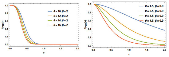
Figure 1. Plots of the PZD survival function for different parameter values.

Hence, from (3) the corresponding cdf of PZD is given by

$$F_{PZD}(x;\theta ,\beta )=1-\left(1+\frac{\theta x^{\beta }\left(\theta +2+\theta x^{\beta }\right)}{\theta +2}\right)e^{-\theta x^{\beta }},x>0,\theta >0,\beta >0.$$

(3)

It is clear that for $\beta =1$, the PZD reduces to the ZD. Plots of the PZD cdf for some selections of $\beta$ and $\theta$ are presented in Figure 2. It is noted that the cdf shapes of the PZD vary with the distribution parameter values.

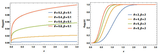
Figure 2. Plots of the cdf of PZD for selected values of $\beta$ and $\theta$.

The pdf of the PZD can be obtained by taking the derivative of $F_{PZD}(x;\theta ,\beta )$ as

$$f_{PZD}(x;\beta ,\theta )=\frac{\beta {\theta }^3}{2+\theta }{x}^{2\beta -1}\left(1+x^{\beta }\right){\mathrm{e}}^{-\theta x^{\beta }},x>0,\theta >0,\beta >0.$$

(4)

Different PZD pdf plots are given in Figure 3 with various parameters. The suggested distribution pdf is asymmetric, unimodal, semi-symmetric ($\theta =8$,$\beta =5$), increasing–decreasing ($\theta =16$,$\beta =1.5$), skewed to the left ($\theta =0.2$,$\beta =5$), and skewed to the right ($\theta =5$,$\beta =0.8$), according to the parameter’s values.

Figure 3. Pdf plots of the PZD with various values of parameters.

The Mode PZD

The logarithm of the PZD pdf given in Equation (4) is

$$log\left[f_{PZD}(x;\beta ,\theta )\right]=log\left(\frac{\beta {\theta }^3}{2+\theta }\right)+(2\beta -1)\log (x)+\log \left(1+x^{\beta }\right)-\theta x^{\beta }.$$

The first derivative of this equation with respect to x is

$$\frac{\partial log\left[f_{PZD}(x;\beta ,\theta )\right]}{\partial x}=\frac{2\beta +x^{\beta }\left[-\left(\beta \left(\theta +\theta x^{\beta }-3\right)+1\right)\right]-1}{x\left(x^{\beta }+1\right)}$$

Let $\frac{\partial log\left[f_{PZD}(x;\beta ,\theta )\right]}{\partial x}=0$ to obtain the mode of the distribution as

$$x_0={\left(\frac{-1+3\beta -\beta \theta +\sqrt{-4\left(1-2\beta \right)\beta \theta +{\left(1-3\beta +\beta \theta \right)}^2}}{2\beta \theta }\right)}^{\frac{1}{\beta }}.$$

3. Statistical Properties

In this section, some of the main statistical properties of the PZD are derived and some simulations are provided.

3.1. Moments

The rth moment about the origin of the PZD is defined as

$$E\left(X_{PZD}^r\right)=\frac{\beta (\theta +2)+r}{\beta (\theta +2)}{\theta }^{-\frac{r}{\beta }}\Gamma \left(\frac{r}{\beta }+2\right),r=1,2,3,...$$

(5)

and hence the mean of the distribution is

$$E\left(X_{PZD}^{}\right)=\frac{\beta (\theta +2)+1}{\beta (\theta +2){\theta }^{\frac{1}{\beta }}}\Gamma \left(\frac{1}{\beta }+2\right)$$

The inverse moment of the PZD is

$$E\left(\frac{1}{X_{PZD}^r}\right)=\frac{\beta (\theta +2)-r}{\beta (\theta +2)}{\theta }^{r/\beta }\Gamma \left(2-\frac{r}{\beta }\right),r=1,2,3,...$$

(6)

While kurtosis of a random variable measures the degree of tail heaviness, skewness of a random variable measures the degree of long-tail. The coefficient of skewness $\left({ƛ}_1\right)$, coefficient of variation $\left({ƛ}_2\right)$, and coefficient of kurtosis $\left({ƛ}_3\right)$ of the PZD are given, respectively, by

$${ƛ}_1=\frac{\begin{array}{l}{\beta }^2{(\theta +2)}^2\left[\beta (\theta +2)+3\right]\Gamma \left(2+\frac{3}{\beta }\right)+2{\left[\beta (\theta +2)+1\right]}^3\Gamma {\left(2+\frac{1}{\beta }\right)}^3\\ -3\beta (\theta +2)\left[\beta (\theta +2)+1\right]\left[\beta (\theta +2)+2\right]\Gamma \left(2+\frac{2}{\beta }\right)\Gamma \left(2+\frac{1}{\beta }\right)\end{array}}{{\left(\beta (\theta +2)\left[\beta (\theta +2)+2\right]\Gamma \left(2+\frac{2}{\beta }\right)-{\left[\beta (\theta +2)+1\right]}^2\Gamma {\left(2+\frac{1}{\beta }\right)}^2\right)}^{3/2}}$$

(7)

$${ƛ}_2=\frac{\sqrt{\beta (\theta +2)\left[\beta (\theta +2)+2\right]\Gamma \left(2+\frac{2}{\beta }\right)-{\left[\beta (\theta +2)+1\right]}^2\Gamma {\left(2+\frac{1}{\beta }\right)}^2}}{\left[\beta (\theta +2)+1\right]\Gamma \left(2+\frac{1}{\beta }\right)}$$

(8)

$${ƛ}_3=\frac{A_1-A_2-A_3}{{\left({\left[\beta (\theta +2)+1\right]}^2\Gamma {\left(2+\frac{1}{\beta }\right)}^2-\beta (\theta +2)\left[\beta (\theta +2)+2\right]\Gamma \left(2+\frac{2}{\beta }\right)\right)}^2}$$

(9)

where

$$A_1={\beta }^3{(\theta +2)}^3\left[\beta (\theta +2)+4\right]\Gamma \left(2+\frac{4}{\beta }\right),$$

$$A_2=4{\beta }^2{(\theta +2)}^2\left[\beta (\theta +2)+1\right]\left[\beta (\theta +2)+3\right]\Gamma \left(2+\frac{3}{\beta }\right)\Gamma \left(2+\frac{1}{\beta }\right),$$

$$A_3=3{\left[\beta (\theta +2)+1\right]}^2\Gamma {\left(2+\frac{1}{\beta }\right)}^2\left\{{\left[\beta (\theta +2)+1\right]}^2\Gamma {\left(2+\frac{1}{\beta }\right)}^2+2\beta (\theta +2)\left[\beta (\theta +2)+2\right]\Gamma \left(2+\frac{2}{\beta }\right)\right\}.$$

Table 1 gives the mean $\left({\mu }_X\right)$, standard deviation $\left({\sigma }_X\right)$, ${ƛ}_1$, ${ƛ}_2$, and ${ƛ}_3$ of the PZD for various selections of the parameters.

Table 1. Values of ${\mu }_X,{\sigma }_X,{ƛ}_1,{ƛ}_2,{ƛ}_3$ for the PZD for selected parameters.

$\mathit{\theta }$	${\mathit{\mu }}_{\mathit{X}}$	${\mathit{\sigma }}_{\mathit{X}}$	${\mathit{ƛ}}_{\mathbf{1}}$	${\mathit{ƛ}}_{\mathbf{2}}$	${\mathit{ƛ}}_{\mathbf{3}}$	$\mathit{\beta }$	${\mathit{\mu }}_{\mathit{X}}$	${\mathit{\sigma }}_{\mathit{X}}$	${\mathit{ƛ}}_{\mathbf{1}}$	${\mathit{ƛ}}_{\mathbf{2}}$	${\mathit{ƛ}}_{\mathbf{3}}$
			$\mathit{\beta }\mathbf{=}\mathbf{3}$						$\mathit{\theta }\mathbf{=}\mathbf{2}$
3	0.881	0.211	0.239	0.003	2.856	4.0	1.012	0.181	0.179	−0.195	2.977
3.1	0.870	0.208	0.239	0.004	2.855	4.1	1.012	0.177	0.175	−0.209	2.990
3.2	0.860	0.206	0.240	0.006	2.854	4.2	1.011	0.173	0.171	−0.222	3.002
3.3	0.850	0.204	0.240	0.007	2.853	4.3	1.010	0.169	0.167	−0.234	3.015
3.4	0.841	0.202	0.240	0.009	2.853	4.4	1.010	0.165	0.163	−0.246	3.028
3.5	0.832	0.200	0.241	0.010	2.852	4.5	1.009	0.161	0.160	−0.258	3.041
3.6	0.823	0.198	0.241	0.011	2.852	4.6	1.009	0.158	0.157	−0.269	3.054
3.7	0.815	0.196	0.241	0.013	2.851	4.7	1.008	0.155	0.153	−0.280	3.067
3.8	0.807	0.195	0.241	0.014	2.851	4.8	1.008	0.152	0.150	−0.290	3.080
3.9	0.799	0.193	0.241	0.015	2.851	4.9	1.008	0.149	0.147	−0.300	3.093

The results in Table 1 indicate that the distribution is skewed to the right for these parameter value selections, with relatively small values of skewness. In addition, it is noted that the mean and variance values are decreasing as one parameter’s values are increasing for a fixed value of the other parameter.

3.2. Order Statistics

Let $X_1,X_2,...,X_m$ be a random sample selected from PZD with cdf (4) and pdf (5) and $X_{(1)},$ $X_{(2)},...,X_{(m)}$ be its order statistics; then, the pdf of the ith $\left(i=1,2,...,m\right)$ order statistic, $X_{(i)}$, is given by

$$\begin{gathered} f_{(i)}(x;\theta ,\beta )=\frac{m!}{(i-1)!(m-i)!}{[F(x;\theta ,\beta )]}^{i-1}{[S(x;\theta ,\beta )]}^{m-i}f(x;\theta ,\beta ) \\ \begin{array}{l}\\ =\frac{\beta {\theta }^{3}m!x^{2\beta -1}\left(x^{\beta }+1\right)e^{-\theta i{x}^{\beta }}{\left[\frac{\theta x^{\beta }\left(\theta +\theta x^{\beta }+2\right)+\theta +2}{\theta +2}\right]}^i{\left[\theta +2-e^{-\theta x^{\beta }}\left(\theta x^{\beta }\left(\theta +\theta x^{\beta }+2\right)+\theta +2\right)\right]}^{m-i}}{\Gamma (i)\Gamma (1-i+m){\left(\theta +2\right)}^m\left[\theta +\theta x^{\beta }\left(\theta +\theta x^{\beta }+2\right)+2\right]}\end{array} \end{gathered}$$

(10)

For $i=1$ and m in (12), the pdfs of the smallest and largest order statistics, respectively, are given by

$$f_{(1)}(x;\theta ,\beta )=\frac{\beta {\theta }^{3}m{x}^{2\beta -1}\left(x^{\beta }+1\right)e^{-\theta x^{\beta }}{\left\{\theta +2-\left[\theta x^{\beta }\left(\theta +\theta x^{\beta }+2\right)+\theta +2\right]e^{-\theta x^{\beta }}\right\}}^{m-1}}{{\left(\theta +2\right)}^m},$$

and

$$f_{(m)}(x;\theta ,\beta )=\frac{\beta {\theta }^{3}m{x}^{2\beta -1}\left(x^{\beta }+1\right)e^{-m\theta x^{\beta }}{\left[\theta x^{\beta }\left(\theta +\theta x^{\beta }+2\right)+\theta +2\right]}^{m-1}}{{\left(\theta +2\right)}^m}.$$

Figure 4 represents the three-dimensional plots of the minimum and maximum pdfs with $m=5$, $\beta =2$ and $1\le \theta \le 4$.

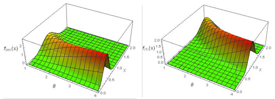
Figure 4. Three-dimensional plots of maximum and minimum pdf of the PZD for $m=5,\beta =2$.

3.3. Reliability Measures

The reliability and hazard functions of any lifetime equipment are the fundamental tools for analyzing aging and associated features. The conditional probability of failure, assuming it has lasted up to time $x\ge 0$, is represented by the hazard function. The hazard, reversed hazard rate, and odds functions of the PZD are given, respectively, by

$$H_{PZD}(x;\theta ,\beta )=\frac{f_{PZD}(x;\theta ,\beta )}{S_{PZD}(x;\theta ,\beta )}=\frac{\beta {\theta }^3{x}^{2\beta -1}\left(x^{\beta }+1\right)}{\theta +\theta x^{\beta }\left(\theta +\theta x^{\beta }+2\right)+2},$$

(11)

$$R{H}_{PZD}(x;\theta ,\beta )=\frac{f_{PZD}(x;\theta ,\beta )}{F_{PZD}(x;\theta ,\beta )}=\frac{\beta {\theta }^3{x}^{2\beta -1}\left(x^{\beta }+1\right)}{(\theta +2)e^{\theta x^{\beta }}-\left(\theta +2+\theta x^{\beta }\left(\theta +\theta x^{\beta }+2\right)\right)},$$

(12)

$$O_{PZD}(x;\theta ,\beta )=\frac{F_{PZD}(x;\theta ,\beta )}{S_{PZD}(x;\theta ,\beta )}=\frac{{\mathrm{e}}^{x^{\beta }\theta }\left(2+\theta \right)}{2+\theta +x^{\beta }\theta \left(2+\theta +x^{\beta }\theta \right)}-1.$$

(13)

Plots of the hazard, reversed hazard rate, and odds functions of the PZD are illustrated in Figure 5, Figure 6, and Figure 7, respectively.

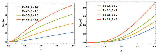
Figure 5. The hazard function plots of PZD for various values of parameters.

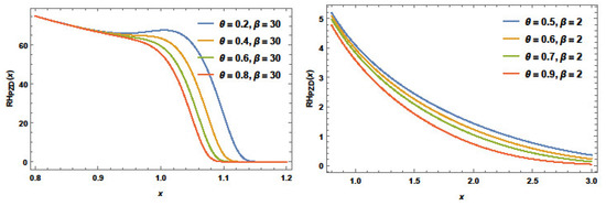
Figure 6. The RHF plots of PZD for various values of parameters.

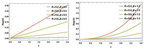
Figure 7. The odds function plots of PZD for selected values of parameters.

Mean residual life (MRL) is crucial in demography, reliability, and survival analysis. The mean residual life function of PZD is defined as

$$\begin{array}{ll}MR{L}_{PZD}(x;\theta ,\beta )& =E(X-x|X>x)=\frac{1}{1-F_{PZD}(x;\theta ,\beta )}{\displaystyle \underset{x}{\overset{\infty }{\mathsf{\int }}}\left(1-F_{PZD}(t;\theta ,\beta )\right)}dt\\ & =\frac{e^{\theta x^{\beta }}\left[\left((\theta +2)\Gamma \left(1+\frac{1}{\beta },x^{\beta }\theta \right)+\Gamma \left(2+\frac{1}{\beta },x^{\beta }\theta \right)+(\theta +2)\Gamma \left(\frac{1}{\beta },x^{\beta }\theta \right)\right)\right]}{\beta {\theta }^{1/\beta }\left[\theta +\theta x^{\beta }\left(\theta +\theta x^{\beta }+2\right)+2\right]}.\end{array}$$

(14)

MRL plots of the PZD for some particular parameters are offered in Figure 8. This figure reveals that the MRL for PZD is decreasing for these values with different behavior decreasing–constant $\left(\theta =8,\beta =0.6\right)$ and decreasing $\left(\theta =2,\beta =3\right)$.

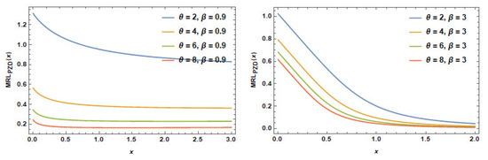
Figure 8. The MRL plots of PZD for selected values of $\theta ,\beta$.

Remark 1. 

It is to be noted that$MR{L}_{PZD}(0;\theta ,\beta )=\mu =\frac{\beta (\theta +2)+1}{\beta (\theta +2){\theta }^{1/\beta }}\Gamma \left(2+\frac{1}{\beta }\right)$.

3.4. Mean and Median Deviations

The mean deviations from the mean and median, which are both essential measurements of the scatter in the population, are defined as

$$\begin{array}{l}{𝒦}_{\mu }={\displaystyle \underset{0}{\overset{\mu }{\int }}(\mu -x)f(x)dx}+{\displaystyle \underset{\mu }{\overset{\infty }{\int }}(x-\mu )f(x)dx}=2\mu F(\mu )-2{\displaystyle \underset{0}{\overset{\mu }{\int }}xf(x)dx}\\ =\frac{2\mu }{\beta {(\theta +2)}^2}\left(\begin{array}{l}{(\theta \mu )}^{-1/\beta }\left[\theta \Gamma \left(2+\frac{1}{\beta },\theta {\mu }^{\beta }\right)+\Gamma \left(3+\frac{1}{\beta },\theta {\mu }^{\beta }\right)-\theta \Gamma \left(2+\frac{1}{\beta }\right)-\Gamma \left(3+\frac{1}{\beta }\right)\right]\\ -\left[\theta \left(\theta {\mu }^{\beta }+\theta +2\right){\mu }^{\beta }+\theta +2\right]{\mathrm{e}}^{-\theta {\mu }^{\beta }}+\theta +2\end{array}\right)\end{array}$$

(15)

and

$$\begin{array}{c}{𝒦}_m={\displaystyle \underset{0}{\overset{m}{\int }}(m-x)f(x)dx}+{\displaystyle \underset{m}{\overset{\infty }{\int }}(x-m)f(x)dx}=\mu -2{\displaystyle \underset{0}{\overset{m}{\int }}xf(x)dx}\\ =\frac{2\beta \left[\theta \Gamma \left(2+\frac{1}{\beta },m^{\beta }\theta \right)+\Gamma \left(3+\frac{1}{\beta },m^{\beta }\theta \right)\right]-\left[\beta (\theta +2)+1\right]\Gamma \left(2+\frac{1}{\beta }\right)}{\beta (\theta +2){\theta }^{1/\beta }},\end{array}$$

(16)

where $\mu =\frac{\beta (\theta +2)+1}{\beta (\theta +2){\theta }^{1/\beta }}\Gamma \left(2+\frac{1}{\beta }\right)$ and m is the population median.

3.5. Quantile Function and Stochastic Ordering

In this section, the quantile function and stochastic ordering are presented and discussed.

3.5.1. Quantile Function

Let $X\sim f_{PZD}(x;\beta ,\theta )$ given in (4). The quantile function, say $Q(p)$, $0<p<1$ defined by $F\left(Q(p)\right)=p$, is the root of the equation

$$\ln \left(\theta +2+\theta Q{(p)}^{\beta }\left(\theta +2+\theta Q{(p)}^{\beta }\right)\right)-\theta Q{(p)}^{\beta }=\ln (1-p)+\ln (\theta +2)$$

(17)

Table 2 presents some quantile values for some choices of p where the real and positive roots are assigned. It can be noted that the $Q(p)$ values are increasing in p.

Table 2. Values for some selected values of p.

p	$\mathit{\theta }\mathbf{=}\mathbf{2}$$\mathbf{,}\mathit{\beta }\mathbf{=}\mathbf{4}$	$\mathit{\theta }\mathbf{=}\mathbf{3}$$\mathbf{,}\mathit{\beta }\mathbf{=}\mathbf{3}$	$\mathit{\theta }\mathbf{=}\mathbf{7}$$\mathbf{,}\mathit{\beta }\mathbf{=}\mathbf{5}$	$\mathit{\theta }\mathbf{=}\mathbf{0.5}$$\mathbf{,}\mathit{\beta }\mathbf{=}\mathbf{0.8}$
0.1	0.77493	0.60731	0.61184	2.14411
0.2	0.86098	0.70059	0.66758	3.43875
0.25	0.89311	0.73638	0.68827	4.05443
0.30	0.92166	0.76861	0.70656	4.67193
0.40	0.97244	0.82687	0.73904	5.95421
0.50	1.01894	0.88125	0.76862	7.36366
0.60	1.06452	0.93544	0.79746	8.99532
0.70	1.11224	0.99309	0.82749	11.0074
0.75	1.13820	1.02484	0.84376	12.2477
0.80	1.16675	1.06003	0.86158	13.7405
0.90	1.24005	1.15175	0.90702	18.2684
0.95	1.29868	1.22643	0.94301	22.7118
0.99	1.40436	1.36385	1.00707	32.9481

3.5.2. Stochastic Ordering

To define the stochastic ordering, a random variable X is smaller than a random variable Y in the following:

(1)

Mean residual life order $(X\underset{MRLO}{\le }Y)$, if $m_X(t)\le m_Y(t)$ for all t.

(2)

Likelihood ratio order $(X\underset{LRO}{\le }Y)$, if $\frac{f_X(t)}{f_Y(t)}$ decreases for all t.

(3)

Hazard rate order $(X\underset{HRO}{\le }Y)$, if $h_X(t)\ge h_Y(t)$ for all t.

(4)

Stochastic order $(X\underset{SO}{\le }Y)$, if $F_X(t)\le F_Y(t)$ for all t.

Remark 2. 

$X\underset{LRO}{\le }Y\Rightarrow X\underset{\underset{X\underset{SO}{\le }Y}{{\displaystyle \Downarrow }}}{\underset{HRO}{\le }}Y\Rightarrow X\underset{MRLO}{\le }Y$.

Theorem 1. 

Let$X_{PZD}\sim f_{XPZD}(t;\beta ,\theta )$and$Y_{PZD}\sim f_{YPZD}(t;\alpha ,\upsilon )$be two random variables. If ($\beta >\alpha$,$\forall \theta ,\upsilon$), or ($\beta =\alpha$with$\theta >\upsilon$), then$X\underset{LRO}{\le }Y$, and thus$X\underset{HRO}{\le }Y$,$X\underset{MRLO}{\le }Y$and$X\underset{SO}{\le }Y$.

Proof. 

Let $X_{PZD}\sim f_{XPZD}(x;\beta ,\theta )$ and $Y_{PZD}\sim f_{YPZD}(x;\alpha ,\upsilon )$. Therefore,

$$\frac{f_{XPZD}(t;\beta ,\theta )}{f_{YPZD}(t;\alpha ,\upsilon )}=\frac{\frac{\beta {\theta }^3}{2+\theta }{t}^{2\beta -1}\left(1+t^{\beta }\right){\mathrm{e}}^{-\theta t^{\beta }}}{\frac{\alpha {\upsilon }^3}{2+\upsilon }{t}^{2\alpha -1}\left(1+t^{\alpha }\right){\mathrm{e}}^{-\upsilon t^{\alpha }}.}=\frac{\beta {\theta }^3\left(2+\upsilon \right)}{\alpha {\upsilon }^3\left(2+\theta \right)}\frac{t^{2\beta -1}\left(1+t^{\beta }\right)}{t^{2\alpha -1}\left(1+t^{\alpha }\right)}{e}^{-(\theta t^{\beta }-\upsilon t^{\alpha })}.$$

For simplification, we have

$$\ln \frac{f_{XPZD}(t;\beta ,\theta )}{f_{YPZD}(t;\alpha ,\upsilon )}=\ln \left(\frac{\beta {\theta }^3\left(2+\upsilon \right)}{\alpha {\upsilon }^3\left(2+\theta \right)}\right)+\ln \left(t^{2\beta -2\alpha }\right)+\ln \left(\frac{1+t^{\beta }}{1+t^{\alpha }}\right)-(\theta t^{\beta }-\upsilon t^{\alpha })$$

Thus,

$$\frac{\partial }{\partial t}\ln \frac{f_{XPZD}(t;\beta ,\theta )}{f_{YPZD}(t;\alpha ,\upsilon )}=\frac{\beta \left(3-\frac{1}{1+t^{\beta }}-t^{\beta }\theta \right)+\alpha \left(-3+\frac{1}{1+t^{\alpha }}+t^{\alpha }\upsilon \right)}{t}$$

To this end, if ($\beta >\alpha$, $\forall \theta ,\upsilon$), or ($\beta =\alpha$ with $\theta >\upsilon$), then $\frac{\partial }{\partial t}\ln \left(\frac{f_{XPZD}(t;\beta ,\theta )}{f_{YPZD}(t;\alpha ,\upsilon )}\right)<0.$ This shows that $X\underset{LRO}{\le }Y$, and according to Remark 2, the theorem is proved. □

3.6. Some Curves and Gini Index

Assume that X is a continuous random variable with a non-negative, twice-differentiable cumulative distribution function. The Bonferroni curve of the random variable X is defined as

$$B(p)=\frac{1}{p\mu } \left(\mu -\underset{q}{\overset{\infty }{\int }}xf(x)dx\right)=\frac{\left[\beta (\theta +2)+1\right]\Gamma \left(2+\frac{1}{\beta }\right)-\beta \left[\theta \Gamma \left(2+\frac{1}{\beta },q^{\beta }\theta \right)+\Gamma \left(3+\frac{1}{\beta },q^{\beta }\theta \right)\right]}{p\left[\beta (\theta +2)+1\right]\Gamma \left(2+\frac{1}{\beta }\right)},$$

(18)

$q=F^{-1}(p)$ and $p\in (0,1]$, and the Lorenz curve is given as

$$L(p)=\frac{1}{\mu } \left(\mu -\underset{q}{\overset{\infty }{\int }}xf(x)dx\right)=1-\frac{\beta \left[\theta \Gamma \left(2+\frac{1}{\beta },q^{\beta }\theta \right)+\Gamma \left(3+\frac{1}{\beta },q^{\beta }\theta \right)\right]}{\left[\beta (\theta +2)+1\right]\Gamma \left(2+\frac{1}{\beta }\right)}, q=F^{-1}(p).$$

(19)

The Gini index of the PZD can be expressed as

$$\begin{array}{ll}GI& =1-\frac{1}{\mu } \underset{0}{\overset{\infty }{\int }}{\left(1-F(x)\right)}^{2}dx\\ & =1-\frac{2^{-\frac{1}{\beta }-4}(\beta +1)\left\{\beta \left[2\beta \left(8\beta {(\theta +2)}^2+2\theta (\theta +8)+27\right)+4\theta +13\right]+1\right\}\Gamma \left(\frac{1}{\beta }\right)}{{\beta }^4(\theta +2)\left[\beta (\theta +2)+1\right]\Gamma \left(2+\frac{1}{\beta }\right)}\end{array}$$

(20)

4. Methods of Estimation and Test

As is well known, the properties of maximum likelihood estimators are not always verified for small samples. Therefore, in recent years, classical and new estimation methods have been developed. One purpose of this work is to investigate different methods to estimate the unknown distribution parameters of the new model, such as maximum likelihood estimation (MLE), ordinary least square (LS), weighted least square (WLS), maximum product of spacing (MPS), Cramer–von Mises estimation (CME), and Anderson–Darling estimation (ADE) methods based on the empirical function distribution. In addition, the Nikulin–Rao–Robson test is considered in this section.

4.1. The MLE

Because of their properties, the maximum likelihood estimators are preferred in providing the values of the unknown parameters. Considering $x_1,x_2,...x_n$ to be a random sample following the $\mathrm{PZD}$ with parameters $\Psi =\left(\theta ,\beta \right)$, the log-likelihood function becomes

$$\log L=n\ln \left(\beta \right)+3n\ln \left(\theta \right)-n\ln \left(2+\theta \right)+\left(2\beta -1\right){\sum }_{i=1}^n\ln \left(x_i\right)+{\sum }_{i=1}^n\ln \left(1+x_i^{\beta }\right)-\theta {\sum }_{i=1}^n{x}_i^{\beta }$$

The maximum likelihood estimators $\widehat{\theta }$ and $\widehat{\beta }$ of the unknown parameters $\theta$ and $\beta ,$ respectively, can be obtained from the following nonlinear score equations as

$$\frac{\partial \log L}{\partial \theta }=0\Rightarrow \frac{3n}{\theta }-\frac{n}{2+\theta }-{\displaystyle \sum _{i=1}^n{x}_i^2}=0.$$

Hence,

$$\widehat{\theta }\left(\widehat{\beta }\right)=\frac{\sqrt{4n\left({\displaystyle \sum _{i=1}^n{x}_i^{\widehat{\beta }}}\right)+{\left({\displaystyle \sum _{i=1}^n{x}_i^{\widehat{\beta }}}\right)}^2+n^2}-{\displaystyle \sum _{i=1}^n{x}_i^{\widehat{\beta }}}+n}{{\displaystyle \sum _{i=1}^n{x}_i^{\widehat{\beta }}}}.$$

(21)

In addition,

$$\frac{\partial \log L}{\partial \beta }=0\Rightarrow \frac{n}{\beta }+2{\sum }_{i=1}^n\ln \left(x_i\right)+{\sum }_{i=1}^n\frac{x_i^{\beta }\ln \left(x_i\right)}{1+x_i^{\beta }}-\theta {\sum }_{i=1}^n{x}_i^{\beta }\ln \left(x_i\right)=0.$$

(22)

The simultaneous solution of the above likelihood equations constitutes the MLEs of $\theta$ and $\beta$. However, analytical solutions are not feasible. Therefore, using R Core Team [21] software, we approximated the solution to the aforementioned normal equations. In addition, we have

$$\frac{{\partial }^2\log L}{\partial {\beta }^2}=-\theta {\displaystyle \sum _{i=1}^n{x}_i^{\beta }}{\log }^2\left(x_i\right)+{\displaystyle \sum _{i=1}^n\left(\frac{x_i^{\beta }{\log }^2\left(x_i\right)}{x_i^{\beta }+1}-\frac{x_i^{2\beta }{\log }^2\left(x_i\right)}{{\left(x_i^{\beta }+1\right)}^2}\right)}-\frac{n}{{\beta }^2}<0,$$

and

$$\frac{{\partial }^2\log L}{\partial {\beta }^2}=-\theta {\displaystyle \sum _{i=1}^n{x}_i^{\beta }}{\log }^2\left(x_i\right)+{\displaystyle \sum _{i=1}^n\left(\frac{x_i^{\beta }{\log }^2\left(x_i\right)}{x_i^{\beta }+1}-\frac{x_i^{2\beta }{\log }^2\left(x_i\right)}{{\left(x_i^{\beta }+1\right)}^2}\right)}-\frac{n}{{\beta }^2}<0,$$

$$\frac{{\partial }^2\log L}{\partial {\theta }^2}=\frac{n}{{(\theta +2)}^2}-\frac{3n}{{\theta }^2}<0.$$

4.2. Methods of LS and WLS

As the explicit forms of the maximum likelihood estimators cannot be obtained every time, some other methods are developed to overcome this problem. The LS and the WLS are well-known methods used for estimating unknown parameters [22]. Here, we consider these two approaches for estimating the unknown parameters of the $PZD$. Let $x_{1,}{x}_{2,\dots },x_n$ be the ordered observations obtained from a sample of size $n$ from the $PZD$. By calculating the minimum of the function

$$S\left(\Psi \right)={\sum }_{i=1}^n{\eta }_i{\left\{1-\left(1+\frac{\theta x_i^{\beta }\left(\theta +2+\theta x_i^{\beta }\right)}{2+\theta }\right)e^{-\theta x_i^{\beta }}-\frac{i}{n+1}\right\}}^2$$

(23)

with respect to $\theta$ and $\beta ,$ respectively, the LS estimates ${\widehat{\theta }}_{LSE}$ and ${\widehat{\beta }}_{LSE}$ can be obtained by setting ${\eta }_i=1$, while we can obtain the $\mathrm{WLS}$ estimates ${\widehat{\theta }}_{WLS}$ and ${\widehat{\beta }}_{WLS}$ by setting ${\eta }_i=\frac{{(n+1)}^2\left(n+2\right)}{i\left(n-i+1\right)}.$ The following equations can be solved to yield these estimates as well as

$$\frac{\partial S\left(\Psi \right)}{\partial \theta }={\sum }_{i=1}^n{\eta }_i\left\{1-\left(1+\frac{\theta x_i^{\beta }\left(\theta +2+\theta x_i^{\beta }\right)}{2+\theta }\right)e^{-\theta x_i^{\beta }}-\frac{i}{n+1}\right\}{\phi }_1\left(x_i,\Psi \right)=0,$$

$$\frac{\partial S\left(\Psi \right)}{\partial \beta }={\sum }_{i=1}^n{\eta }_i\left\{1-\left(1+\frac{\theta x_i^{\beta }\left(\theta +2+\theta x_i^{\beta }\right)}{2+\theta }\right)e^{-\theta x_i^{\beta }}-\frac{i}{n+1}\right\}{\phi }_2\left(x_i,\Psi \right)=0,$$

where

$${\phi }_1\left(x_i,\Psi \right)=\frac{\left(\theta x_i^{\beta }+2x_i^{\beta }+\theta +3\right){\theta }^2{x}_i^{2\beta }{e}^{-\theta x_i^{\beta }}}{2+\theta },\mathrm{and}{\phi }_2\left(x_i,\Psi \right)=\frac{\left(1+x_i^{\beta }\right){\theta }^3{x}_i^{2\beta }\ln \left(x_i\right)e^{-\theta x_i^{\beta }}}{2+\theta }.$$

4.3. Method of Maximum Product of Spacing

According to [23], and based on the differences among the values of the cdf at successive data points, the maximum product of spacing is an estimation method as interesting as that of MLE. Moreover, ref. [24] concluded that the $\mathrm{MPS}$ estimator method outperforms all the other estimator methods.

The uniform spacings can be defined using a random sample of size n from a distribution with cdf $F\left(x_i,\Psi \right)$ as follows:

$$D_i\left(\Psi \right)=F\left(x_i,\Psi \right)-F\left(x_{i-1},\Psi \right),i=1,2,...,n$$

where $F\left(x_0,\Psi \right)=0$ and $F\left(x_{n+1},\Psi \right)=1$. The $\mathrm{MPS}$ estimates denoted by ${\widehat{\theta }}_{MPS}$ and ${\widehat{\beta }}_{MPS}$ maximize the function $M\left(\Psi \right)$ with respect to the unknown parameters $\theta$ and $\beta$ as

$$\begin{gathered} M\left(\Psi \right)=\frac{1}{n+1}{\sum }_{i=1}^{n+1}\log D_i\left(\Psi \right)= \\ \frac{1}{n+1}{\displaystyle \sum }_{i=1}^{n+1}\log \left\{e^{-\theta x_{i-1}^{\beta }}\left(1+\frac{\theta x_{i-1}^{\beta }\left(\theta +2+\theta x_{i-1}^{\beta }\right)}{2+\theta }\right)-e^{-\theta x_i^{\beta }}\left(1+\frac{\theta x_i^{\beta }\left(\theta +2+\theta x_i^{\beta }\right)}{2+\theta }\right)\right\}, \end{gathered}$$

or by solving the subsequent equations

$$\frac{\partial M\left(\Psi \right)}{\partial \theta }=\frac{1}{n+1}{\displaystyle \sum }_{i=1}^{n+1}\frac{{\phi }_1\left(x_{i-1},\Psi \right)-{\phi }_1\left(x_i,\Psi \right)}{D_i}=0,$$

$$\frac{\partial M\left(\Psi \right)}{\partial \beta }=\frac{1}{n+1}{\displaystyle \sum }_{i=1}^{n+1}\frac{{\phi }_2\left(x_{i-1},\Psi \right)-{\phi }_2\left(x_i,\Psi \right)}{D_i}=0,$$

where ${\phi }_1\left(x_i,\Psi \right)$ and ${\phi }_2\left(x_i,\Psi \right)$ are given earlier. For more details on this method, see [25].

4.4. Cramer–Von Mises and Anderson–Darling Methods

In recent years, some authors have used classical GOF statistics such as Cramer–von Mises and Anderson–Darling statistics to derive the estimators of the unknown parameters. Ref. [26] used these methods for the binomial-exponential 2 distributions, while [27] evaluated the process capability index for normal distribution. Aside from these methods and using this approach, we propose the use of the Pearson Chi-square statistic $X^2$ where the estimators noted $CSMM$ are obtained by calculating the minimum of $X^2$ with respect to the unknown parameters.

Ref. [28] and later [29] showed that the Cramer–von Mises estimates based on the distance of Cramer–von Mises GOF statistics are the least biased compared to the other estimators. For calculation purposes, ref. [29] gives the formula $C\left(\Psi \right)$ for this statistic, where the estimators ensure its minimum concerning the unknown parameters, where

$$C\left(\Psi \right)=\frac{1}{12n}+{\sum }_{i=1}^n{\left\{1-\left(1+\frac{\theta x_i^{\beta }\left(\theta +2+\theta x_i^{\beta }\right)}{2+\theta }\right)e^{-\theta x_i^{\beta }}-\frac{2i-1}{2n}\right\}}^2.$$

(24)

They also can be gained as the solution of the subsequent equations:

$$\frac{\partial C\left(\Psi \right)}{\partial \theta }={\sum }_{i=1}^n\left\{1-\left(1+\frac{\theta x_i^{\beta }\left(\theta +2+\theta x_i^{\beta }\right)}{2+\theta }\right)e^{-\theta x_i^{\beta }}-\frac{2i-1}{2n}\right\}{\phi }_1\left(x_i,\Psi \right)=0$$

$$\frac{\partial C\left(\Psi \right)}{\partial \beta }={\sum }_{i=1}^n\left\{1-\left(1+\frac{\theta x_i^{\beta }\left(\theta +2+\theta x_i^{\beta }\right)}{2+\theta }\right)e^{-\theta x_i^{\beta }}-\frac{2i-1}{2n}\right\}{\phi }_2\left(x_i,\Psi \right)=0.$$

The Anderson–Darling estimation method is based on the classical Anderson and Darling $\left(AD\right)$ goodness-of-fit statistic test proposed by [30]. This statistic is essentially used to fit data to a theoretical hypothesized model $F_0\left(x\right).$ When the parameters are unknown, they can be estimated by ${\widehat{\theta }}_{ADE}$, ${\widehat{\beta }}_{ADE}$ which minimize the $AD$ statistic given in the form

$$ADE\left(\Psi \right)=-n-n^{-1}{\displaystyle \sum }_{i=1}^n(2i-1)\left\{\log F\left(x_i\right)+\log \left(1-F\left(x_{-i+n+1}\right)\right)\right\},$$

which is equivalent to canceling the first derivatives of this function with respect to $\beta$ and $\theta$. For more details on this method, see [29]. In their paper, ref. [31] showed that the $ADE$ estimation method gives the most efficient estimators. As is known, the Anderson–Darling statistic gives more weight to the tails of the distribution, so for right- or left-tailed distributions, the $ADE$ right tail ($AD{E}_{R-T})$ and $ADE$ left tail ($AD{E}_{L-T})$ can be considered for estimating the unknown parameters, as in [27,31,32].

The $AD{E}_{R-T}$ estimators of $\theta$ and $\beta$ denoted by ${\widehat{\theta }}_{AD{E}_{\left(R-T\right)}}$, ${\widehat{\beta }}_{AD{E}_{\left(R-T\right)}}$, respectively, are found by minimizing the equation given by

$$AD{E}_{\left(R-T\right)}\left(\Psi \right)=\frac{n}{2}-2{\sum }_{i=1}^n\log F\left(x_i\right)-\frac{1}{n}{\sum }_{i=1}^n(2i-1)\log \left\{1-F\left(x_{-i+n+1}\right)\right\}$$

or

$$\frac{\partial }{\partial \theta }\left[AD{E}_{\left(R-T\right)}\left(\Psi \right)\right]=0,\hspace{1em}\frac{\partial }{\partial \beta }\left[AD{E}_{\left(R-T\right)}\left(\Psi \right)\right]=0$$

Similarly, the $AD{E}_{L-T}$ estimators denoted by ${\widehat{\theta }}_{AD{E}_{\left(L-T\right)}}$, ${\widehat{\beta }}_{AD{E}_{\left(L-T\right)}}$ are acquired by minimizing the equation

$$AD{E}_{\left(L-T\right)}\left(\Psi \right)=-\frac{3}{2}n+2{\sum }_{i=1}^{n}F\left(x_i\right)-\frac{1}{n}{\sum }_{i=1}^n(2i-1)\log \left\{F\left(x_i\right)\right\}$$

or

$$\frac{\partial }{\partial \theta }\left[AD{E}_{\left(L-T\right)}\left(\Psi \right)\right]=0,\hspace{1em}\frac{\partial }{\partial \beta }\left[AD{E}_{\left(L-T\right)}\left(\Psi \right)\right]=0$$

with respect to the unknown distribution parameters. For more about the Anderson–Darling estimators, see [27,31,32]. Conversely, ref. [33] demonstrated that the $ADE$ minimum-distance estimation method is a highly competitive method compared to the $\mathrm{ML}$ estimation. In addition, ref. [24] confirmed the superiority of this method.

4.5. The Nikulin–Rao–Robson Test

The probability distribution used to describe any phenomenon is very important in this analysis. Since the twentieth century, researchers have continued to develop techniques to validate the different models. In addition to the classical procedures, we considered in this work a criteria test statistic based on the Nikulin–Rao–Robson statistic (NRR) to fit data to the $\mathrm{PZD}$. The great interest of the NRR statistic is that it recovers all the information lost while grouping data. Based on the MLE on initial data, this statistic $Y^2$ introduced by [34,35] is a modification of the well-known Chi-square Pearson statistic $T^2$. For testing the null hypothesis $H_0$, given by

$$H_0=P\left(X_i\le x\right)=F\left(x,\Psi \right),x\ge 0.$$

According to the above, the sample $X_1,X_2,\dots , X_n$ belongs to the parametric family $F\left(x,\Psi \right)$ with unknown parameters, and $Y^2$ consists in grouping data into $r$ equiprobable intervals $I_1,I_2,$...$,I_r$, where

$$I_j=\left]a_{j-1},a_j\right];I_i\cap I_j=\varphi i\ne j;\underset{j=1}{\overset{r}{{\displaystyle \cup }}}{I}_j=R^1,$$

such as

$$p_j={\int }_{a_{j-1}}^{a_j}f\left(x,\Psi \right)dx=\frac{1}{r},\hspace{1em}j=1,2,...,r.$$

If $\upsilon ={\left({\upsilon }_1,{\upsilon }_2,...,{\upsilon }_r\right)}^T$ represents the number of observed $X_i$ grouping into these intervals $I_j$, and the vector $T_n\left(\Psi \right)$ is given by

$$T_n\left(\widehat{\Psi }\right)={\left(\frac{v_1-n{p}_1\left(\widehat{\Psi }\right)}{\sqrt{n{p}_1\left(\widehat{\Psi }\right)}},\frac{v_2-n{p}_2\left(\widehat{\Psi }\right)}{\sqrt{n{p}_2\left(\widehat{\Psi }\right)}},\dots ,\frac{v_r-n{p}_r\left(\widehat{\Psi }\right)}{\sqrt{n{p}_r\left(\widehat{\Psi }\right)}}\right)}^t.$$

The NRR statistic $Y^2$ is defined as

$$Y_n^2\left(\widehat{\Psi }\right)=T_n^2\left(\widehat{\Psi }\right)+\frac{1}{n}{l}^T\left(\widehat{\Psi }\right){\left(I\left(\widehat{\Psi }\right)-J\left(\widehat{\Psi }\right)\right)}^{-1}l\left(\widehat{\Psi }\right),$$

where $I\left(\widehat{\Psi }\right)$ and $J\left(\widehat{\Psi }\right)$ are the estimated information matrices on non-grouped and grouped data, respectively, and $\widehat{\Psi }$ is the vector of the ML estimators on initial data. The components of the vector $l\left(\widehat{\Psi }\right)={\left(l_s\left(\widehat{\Psi }\right)\right)}_{1\times s}^t$ and the matrix $J\left(\widehat{\Psi }\right)$ are

$$l_s\left(\widehat{\Psi }\right)={\displaystyle \sum }_{i=1}^r\frac{{\nu }_j}{p_j}\frac{\partial p_j\left(\widehat{\Psi }\right)}{\partial {\widehat{\Psi }}_s},$$

$$J\left(\widehat{\Psi }\right)={\left(\frac{1}{\sqrt{p_j}}\frac{\partial p_j\left(\widehat{\Psi }\right)}{\partial {\widehat{\Psi }}_k}\right)}_{r\times s}^t{\left(\frac{1}{\sqrt{p_j}}\frac{\partial p_j\left(\widehat{\Psi }\right)}{\partial {\widehat{\Psi }}_k}\right)}_{r\times s},j=1,2,\dots ,r\mathrm{and}k=1,2,\dots ,s,$$

where $s$ represents the number of parameters. The distribution of $Y^2\left(\widehat{\Psi }\right)$ is a Chi-square with $r-1$ degrees of freedom. To construct the test statistic $Y^2$ corresponding to the PZD $\left(\widehat{\Psi }\right)$ we calculated the ML estimators $\widehat{\Psi }={(\widehat{\beta },\widehat{\theta })}^t,$ the limit intervals $a_j$, and the derivatives $\frac{\partial p_j\left(\widehat{\Psi }\right)}{\partial {\widehat{\Psi }}_k}$ for our model.

$$\frac{\partial p_j\left(\widehat{\Psi }\right)}{\partial \widehat{\theta }}={\phi }_1\left(x_j,\widehat{\Psi }\right)-{\phi }_1\left(x_{j-1},\widehat{\Psi }\right),\frac{\partial p_j\left(\widehat{\Psi }\right)}{\partial \widehat{\beta }}={\phi }_2\left(x_j,\widehat{\Psi }\right)-{\phi }_2\left(x_{j-1},\widehat{\Psi }\right).$$

Then, after computing the estimated information matrices $I\left(\widehat{\Psi }\right)$ and $J\left(\widehat{\Psi }\right)$, we obtained the statistic $Y^2\left(\widehat{\Psi }\right)$ for the $PZD$ distribution. This method is used to construct GOF test statistics for some generalized models; for examples see [36,37,38,39].

5. Simulations

In this section, we investigate the performance of the estimation procedures used in this paper. To that end, we generated $10,000$ samples with different sizes ($n=10,$ $n=25,$ $n=35,$ $n=75,$ $n=200$, and $n=400)$ from the $PDZ$ model, and then computed the different estimators and their mean square errors (MSE) (values in brackets) for the unknown parameters using R statistical software when $\theta =5$ and $\beta =0.5$. The results are given by sample size in Table 3.

Table 3. Estimators’ values of $\theta =5$ and $\beta =0.5$ with different estimation methods.

	$\mathit{\theta }=5$	$\mathit{\beta }=0.5$	$\mathit{\theta }=5$	$\mathit{\beta }=0.5$
	n = 10		n = 25
MLE	4.8841 (0.0122)	0.5899 (0.0124)	4.8993 (0.0105)	0.5776 (0.0106)
WLS	4.8973 (0.0120)	0.5832 (0.0117)	4.9176 (0.0103)	0.5719 (0.0099)
MPS	4.8812 (0.0136)	0.6118 (0.0147)	4.8935 (0.0119)	0.5995 (0.0129)
CMEs	5.0735 (0.0126)	0.3099 (0.0131)	5.0632 (0.0109)	0.4023 (0.0113)
LSE	5.0759 (0.0098)	0.4244 (0.0093)	5.0607 (0.0086)	0.4355 (0.0085)
ADE	5.1405 (0.0158)	0.3768 (0.0159)	5.1282 (0.0141)	0.3928 (0.0141)
ADEL-R	5.1477 (0.0167)	0.3709 (0.0171)	5.1354 (0.0150)	0.3851 (0.0153)
ADEL-T	5.1656 (0.0175)	0.3653 (0.0177)	5.1533 (0.0158)	0.3782 (0.0159)
	$n=35$		$n=75$
MLE	4.9146 (0.0090)	0.5611 (0.0089)	4.9644 (0.0040)	0.5348 (0.0037)
WLS	4.9391 (0.0088)	0.5567 (0.0082)	4.9271 (0.0079)	0.5445 (0.0070)
MPS	4.9069 (0.0104)	0.5832 (0.0112).	4.9224 (0.0090)	0.5567 (0.0077)
CMEs	5.0517 (0.0094)	0.4152 (0.0096)	5.0364 (0.0072)	0.4274 (0.0061)
LSE	5.0454 (0.0071)	0.4507 (0.0068)	5.0329 (0.0055)	0.4623 (0.0052)
ADE	5.1068 (0.0127)	0.4011 (0.0124)	5.0852 (0.0111)	0.4143 (0.0093)
ADEL-R	5.1143 (0.0136)	0.3980 (0.0136)	5.0924 (0.0120)	0.4112 (0.0099)
ADEL-T	5.1319 (0.0144)	0.3914 (0.0142)	5.1103 (0.0125)	0.4056 (0.0116)
	$n=200$		$n=400$
MLE	4.9869 (0.0027)	0.5123 (0.0024)	4.9989 (0.0012)	0.5003 (0.0009)
WLS	4.9586 (0.0061)	0.5183 (0.0053)	4.9813 (0.0043)	0.5054 (0.0035)
MPS	4.9437 (0.0072)	0.5304 (0.0060)	4.9763 (0.0056)	0.5078 (0.0042)
CMEs	5.0195 (0.0053)	0.5412 (0.0044)	5.0096 (0.0038)	0.4834 (0.0026)
LSE	5.0167 (0.0039)	0.4785 (0.0035)	5.0035 (0.0023)	0.4908 (0.0015)
ADE	5.0527 (0.0093)	0.4408 (0.0076)	5.0234 (0.0077)	0.4733 (0.0058)
ADEL-R	5.0633 (0.0102)	0.4377 (0.0081)	5.0302 (0.0086)	0.4702 (0.0063)
ADEL-T	5.0741 (0.0110)	0.4321 (0.0094)	5.0416 (0.0092)	0.4646 (0.0076)

Based on Table 2, it can be noted that the bias and MSE values of different estimators decrease as the sample size increases. For example, when $\theta =5$ with $n=10$ and $n=400$, the MLE values are $\widehat{\theta }=4.8841$ and $\widehat{\theta }=4.9989$, respectively. In addition, for the same case of $\theta =5$, $n=10$, and $n=400$, the values of the LSE are $\widehat{\theta }=5.0759$ and $\widehat{\theta }=5.0167,$ respectively. In general, we can say that the LSE method performs better than other methods up to $n\le 35$, while the MLE is the best one for $n\ge 75$ in terms of the MSE.

6. Applications

The analysis of three real data sets is considered to show the usefulness of the proposed distribution in modeling different phenomena and the performances of the methods used to determine the unknown parameters. In addition to the traditional model selection techniques, we calculated the $Y^2$ statistic to prove that the proposed model fits some data sets better than some commonly used alternative distributions, such as:

-

The xgamma distribution suggested by [40] with pdf given by

$$f(x;\theta )=\frac{{\theta }^2}{1+\theta }\left(1+\frac{\theta }{2}{x}^2\right)e^{-\theta x},x>0,\theta >0.$$

-

Gamma distribution with pdf given by

$$f(x;\alpha ,\beta )=\frac{1}{{\beta }^{\alpha }\Gamma (\alpha )}{x}^{\alpha -1}{e}^{-\frac{x}{\beta }},x>0,\alpha ,\beta >0.$$

-

Lomax distribution with pdf given by

$$f(x;\alpha ,\lambda )=\frac{\alpha }{\lambda }{\left(1+\frac{x}{\lambda }\right)}^{-(\alpha +1)},x>0,\theta ,\beta >0.$$

-

Darna distribution proposed by [41] with pdf given by

$$f_{DD}(y;\theta ,\alpha )=\frac{\theta }{2{\alpha }^2+{\theta }^2}\left(2\alpha +\frac{{\theta }^4{y}^2}{2{\alpha }^3}\right)e^{-\frac{\theta y}{\alpha }};y>0,\theta >0,\alpha >0,$$

-

Power Darna distribution introduced by [13] with pdf given by

$$f_{PDD}(x;\alpha ,\beta ,\theta )=\frac{\beta \theta }{2{\alpha }^3\left(2{\alpha }^2+{\theta }^2\right)}{x}^{\beta -1}\left(4{\alpha }^4+{\theta }^4{x}^{2\beta }\right)e^{-\frac{\theta x^{\beta }}{\alpha }},x>0,\theta ,\beta ,\alpha >0.$$

-

Power Lindley distribution proposed by [2] with pdf defined as

$$f_{PLD}(x;\beta ,\theta )=\frac{\beta {\theta }^2}{1+\theta }{x}^{\beta -1}\left(1+x^{\beta }\right){\mathrm{e}}^{-\theta x^{\beta }},x>0,\theta ,\beta >0.$$

-

Exponentiated power Lindley distribution (EPLD) offered by [42] with pdf given by

$$f_{EPLD}(x;\beta ,\theta )=\frac{\alpha \beta {\theta }^2{x}^{\beta -1}}{1+\theta }\left(1+x^{\beta }\right){\mathrm{e}}^{-\theta x^{\beta }}{\left[1-\left(1+\frac{\theta x^{\beta }}{1+\theta }\right){\mathrm{e}}^{-\theta x^{\beta }}\right]}^{\alpha -1},x>0,\theta ,\beta >0.$$

6.1. First Data: Failure Times of Devices

The first real data set refers to the failure times of 50 items put under a life test. It is generally known that this data set displays bathtub behavior of the hazard rate function [43]. This data set has been analyzed by many authors. The data are 0.1, 1.0, 1.0, 1.0, 2.0, 3.0, 82.0, 83.0, 84.0, 6.0, 7.0, 11.0, 36.0, 40.0, 45.0, 12.0, 18.0, 18.0, 21.0, 18.0, 0.2, 1.0, 1.0, 18.0, 18.0, 32.0, 45.0, 47.0, 63.0, 63.0, 67.0, 67.0, 50.0, 55.0, 60.0, 67.0, 67.0, 72.0, 85.0, 85.0, 85.0, 85.0, 75.0, 79.0, 82.0, 84.0, 84.0, 85.0, 86.0, 86.0. Figure 9 displays the density, total time on test transform (TTT), probability–probability (P–P) plot, and quantile–quantile (Q–Q) plot of the PZD for the failure times data.

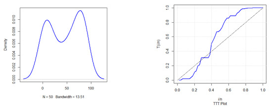
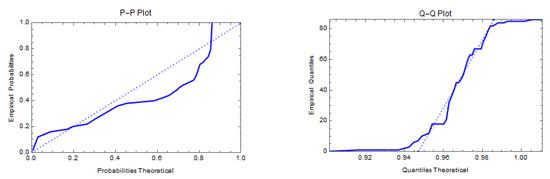
Figure 9. The density, TTT, P–P, and Q–Q plots of the PZD for the failure times data.

Table 4 represents the values of the parameter estimators for the hypothesized distribution $PZD$ obtained by the different methods, and Kolmogorov–Smirnov (KS) and the corresponding p-values. Because $n=50>30,$ it is established by the simulation study that the $MLE$ methods give the best results.

Table 4. Different parameter estimators for failure times data.

Method	$\mathit{\beta }$	$\mathit{\theta }$	KS	p-Value
MLE	0.6763	4.6777	0.1726	0.9496
WLS	0.3646	2.3162	0.1976	0.9284
MPS	0.2346	3.4677	0.2011	0.9202
CMEs	0.3679	5.6626	0.1938	0.9334
LSE	0.5976	4.7647	0.1784	0.9412
ADE	0.6696	6.6133	0.2134	0.9177
ADEL-R	0.8010	7.6727	0.2212	0.9086
ADEL-T	0.9262	8.7689	0.2276	0.9010

As the maximum likelihood parameter estimators for the competing distributions are required to calculate their corresponding NRR test statistic $Y^2$, the MLE values are calculated and given in Table 5.

Table 5. ML parameter estimates for the alternative distributions based on failure times data.

Distributions	Estimates
PZD	$\widehat{\beta }=0.6763$$,\widehat{\theta }=4.6777$
ZD	$\widehat{\theta }=1.7826$
Lomax	$\widehat{\alpha }=2.3467$$,\widehat{\lambda }=1.0934$
Xgamma	$\widehat{\theta }=1.3476$
Gamma	$\widehat{\alpha }=1.7266$$,\widehat{\beta }=0.0839$
Darna	$\widehat{\alpha }=1.6346$$,\widehat{\theta }=2.7682$
Power Lindley	$\widehat{\alpha }=1.6235$$,\widehat{\beta }=2.0145$,
Power Darna	$\widehat{\alpha }=2.856$$,\widehat{\beta }=3.1624$$,\widehat{\theta }=0.0935$
EP LD	$\widehat{\alpha }=8.6321$$,\widehat{\beta }=0.8562$$,\widehat{\theta }=3.4152$

To distinguish between the proposed model and its alternatives, we used classical criteria for model selection, and the NRR statistics with the corresponding values are summarized in Table 6.

Table 6. Values of criteria statistics for model selection based on failure times data.

Distributions	Y2	W	A	K-S (p-Value)	-NLL	AIC	CAIC	BIC
PZD	8.4684	0.2986	0.6844	0.1726 (0.9496)	213.8102	431.6204	431.8757	435.4444
ZD	10.3344	0.4144	0.7468	0.2633 (0.9264)	236.7156	475.4312	475.5145	477.3432
Lomax	10.9816	0.5282	0.7677	0.4476 (0.9103)	253.4021	510.8042	511.0595	514.6282
Xgamma	12.6326	0.5633	0.9436	0.3466 (0.9098)	241.0956	484.1312	484.2145	486.1032
Gamma	11.3392	0.4496	0.8434	0.5233 (0.9126)	262.3364	528.6728	528.9281	532.4968
Darna	9.2204	0.3642	0.6939	0.1833 (0.9312)	221.9302	447.8604	448.1157	451.6844
Power Lindley	12.8596	0.5698	0.9445	0.5325 (0.8965)	268.9236	541.8472	542.1025	545.6710
Power Darna	8.7659	0.3245	0.6862	0.1756 (0.9423)	221.3546	448.7092	449.2309	454.4450
EP LD	13.0251	0.5702	0.9512	0.5366 (0.8902)	272.3256	550.6512	551.1729	556.3870

From Table 6, we can see that the smallest values of the different criteria for model selection are obtained for the PZD, which confirms that the proposed PZD model describes these data better than all the alternatives.

6.2. Second Data: Remission Times

The second case addressed the lengths of remission times (in months) of 128 bladder cancer patients who are randomly selected, as reported by [44]. The data observations are 0.08, 4.87, 6.94, 8.66, 2.09, 3.48, 13.11, 23.63, 0.20, 13.80, 25.74, 0.50, 2.23, 3.52, 4.98, 6.97, 9.02, 3.88, 5.32, 7.39, 10.34, 13.29, 0.40, 2.26, 9.22, 2.46, 3.64, 5.09, 7.26, 0.51, 2.54, 14.76, 26.31, 0.81, 3.70, 5.17, 7.28, 9.47, 14.24, 25.82, 9.74, 2.62, 3.82, 5.32, 2.69, 4.23, 5.41, 7.62, 7.32, 10.06, 14.77, 32.15, 2.64, 14.83, 34.26, 4.33, 5.49, 7.66, 0.90, 5.34, 7.59, 10.66, 15.96, 2.69, 4.18, 36.66, 12.05, 10.75, 16.62, 43.01, 5.41, 7.63, 11.25, 17.14, 79.05, 17.12, 46.12, 4.40, 5.85, 8.26, 1.26, 2.83, 1.35, 2.87, 5.62, 1.19, 2.75, 4.26, 7.87, 11.64, 4.34, 5.71, 7.93, 11.79, 17.36, 1.40, 3.02, 18.10, 1.46, 11.98, 19.13, 12.02, 2.02, 3.31, 1.76, 3.25, 12.03, 20.28, 2.02, 4.50, 6.25, 8.37, 4.51, 6.54, 8.53, 3.36, 6.76, 8.65, 12.63, 22.69, 12.07, 21.73, 3.57, 5.06, 7.09, 2.07, 3.36, 6.93. Figure 10 represents the density, TTT, P–P, and Q–Q plots of the PZD for the 128 bladder cancer patients’ data. Various parameter estimators based on cancer patients’ data are summarized in Table 7.

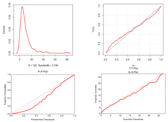
Figure 10. The density, TTT, P–P, and Q–Q plots of the PZD for bladder cancer patients’ data.

Table 7. Different parameter estimators for cancer patients’ data.

Method	$\mathit{\beta }$	$\mathit{\theta }$	KS	p-Value
MLE	0.4342	5.1267	0.0314	0.8434
WLS	0.6764	6.3616	0.0386	0.8383
MPS	0.6989	7.7768	0.0497	0.8198
CMEs	0.4213	4.9674	0.0478	0.8266
LSE	0.3417	4.1625	0.0412	0.8317
ADE	0.7895	8.4616	0.0519	0.8078
ADEL-R	0.7618	8.7786	0.0581	0.7984
ADEL-T	0.8216	9.7633	0.0553	0.8010

As the ML parameter estimators for the competing distributions are needed to compute their corresponding NRR test statistic $Y^2$, the MLE values are calculated and given in Table 8.

Table 8. ML parameter estimates for the alternative distributions based on cancer patients’ data.

Distributions	Estimates
PZD	$\widehat{\beta }=0.4342$$,\widehat{\theta }=5.1267$
ZD	$\widehat{\theta }=2.3461$
Lomax	$\widehat{\alpha }=1.6798$$,\widehat{\lambda }=0.9436$
Xgamma	$\widehat{\theta }=1.9826$
Gamma	$\widehat{\alpha }=2.3639$$,\widehat{\beta }=0.1364$
Darna	$\widehat{\alpha }=0.9671$$,\widehat{\theta }=1.3478$
Power Lindley	$\widehat{\alpha }=1.8963$$,\widehat{\beta }=3.0596$,
Power Darna	$\widehat{\alpha }=3.0614$$,\widehat{\beta }=2.9356$$,\widehat{\theta }=0.1796$
EP LD	$\widehat{\alpha }=5.6947$$,\widehat{\beta }=0.4972$$,\widehat{\theta }=1.7693$

To show that this model can also describe this type of data, we used all classical criteria for model selection and the modified Chi-square NRR. All of the corresponding values are computed and given in Table 9.

Table 9. Values of criteria statistics for model selection based on cancer patients’ data.

Distributions	Y2	A	W	K-S (p-Value)	-NLL	AIC	BIC
PZD	9.8906	0.6782	0.0934	0.0314 (0.8434)	346.3315	696.6630	700.4870
ZD	12.7648	0.7341	0.1598	0.0346 (0.7946)	352.9865	707.9730	709.8850
Darna	10.9636	0.6914	0.1241	0.0324 (0.8126)	349.6614	703.3228	707.1468
Xgamma	13.9246	0.7633	0.1739	0.0377 (0.7767)	354.6978	711.3956	713.3076
Gamma	11.8246	0.7146	0.1433	0.0334 (0.8098)	351.2365	706.4730	710.2970
Lomax	13.0146	0.7424	0.1646	0.0356 (0.7833)	353.6748	711.3496	715.1736
Power Lindley	12.5362	0.8125	0.1762	0.0374 (0.7614)	356.2350	716.4700	722.1740
Power Darna	10.0236	0.6825	0.1143	0.0320 (0.8234)	348.6320	703.2640	711.8200
EP LD	14.5236	0.9125	0.1726	0.0402 (0.7522)	362.2530	730.5060	739.0620

From Table 9, we can see that the smallest values of the different criteria for model selection are obtained for the PZD, which confirms that the proposed model describes these data better than all the alternatives considered here.

6.3. Third Data: Strengths of 1.5 cm Glass Fibers

We then considered the data set representing the strengths of 1.5 cm glass fibers. The data set is also analyzed by [45,46]. The data are 0.55, 0.93, 1.25, 1.36, 1.49, 1.52, 1.58, 1.61, 1.64, 1.68, 1.73, 1.81, 2.00, 0.74, 1.04, 1.27, 1.39, 1.49, 1.53, 1.59, 1.61, 1.66, 1.68, 1.76, 1.82, 2.01, 0.77, 1.11, 1.28, 1.42, 1.50, 1.54, 1.60, 1.62, 1.66, 1.69, 1.76, 1.84, 2.24, 0.81, 1.13, 1.29, 1.48, 1.50, 1.55, 1.61, 1.62, 1.66, 1.70, 1.77, 1.84, 0.84, 1.24, 1.30, 1.48, 1.51, 1.55, 1.61, 1.63, 1.67, 1.70, 1.78, 1.89. Figure 11 represents the density, TTT, P–P, and Q–Q plots of the PZD for the glass fiber data.

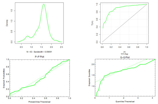
Figure 11. The density, TTT, P–P, and Q–Q plots of the PZD with glass fiber data.

Table 10 represents the values of the parameter estimators for the hypothesized distribution PZD obtained by the different methods and the corresponding p-values.

Table 10. Different parameter estimators with glass fiber data.

Method	$\mathit{\beta }$	$\mathit{\theta }$	KS	p-Value
MLE	0.3152	3.5162	0.0422	0.8496
WLS	0.2365	5.0215	0.0485	0.8377
MPS	0.5326	4.9936	0.0502	0.8222
CMEs	0.4152	3.5162	0.0564	0.8143
LSE	0.3465	4.0321	0.0446	0.8435
ADE	0.2526	4.5136	0.0534	0.8102
ADEL-R	0.0236	2.6351	0.0599	0.7933
ADEL-T	0.1635	3.5162	0.0578	0.8089

As the maximum likelihood parameter estimators for the competing distributions are needed to compute their corresponding NRR test statistic Y², the MLE values are calculated and given in Table 11.

Table 11. ML parameter estimates for the alternative distributions with glass fiber data.

Distributions	Estimates
PZD	$\widehat{\beta }=0.3152$$,\widehat{\theta }=3.5162$
ZD	$\widehat{\theta }=3.5614$
Lomax	$\widehat{\alpha }=2.1635$$,\widehat{\lambda }=0.7263$
Xgamma	$\widehat{\theta }=1.5312$
Gamma	$\widehat{\alpha }=3.1259$$,\widehat{\beta }=0.0985$
Darna	$\widehat{\alpha }=0.8132$$,\widehat{\theta }=1.7452$
Power Lindley	$\widehat{\alpha }=1.3416$$,\widehat{\beta }=1.9236$
Power Darna	$\widehat{\alpha }=1.285$$,\widehat{\beta }=2.6351$$,\widehat{\theta }=0.0632$
EP LD	$\widehat{\alpha }=6.2451$$,\widehat{\beta }=0.7325$$,\widehat{\theta }=4.201$

To show that this model can also describe this type of data, we used all classical criteria for model selection and the modified chi-square NRR. All the corresponding values are computed and given in Table 12.

Table 12. Values of criteria statistics for model selection with glass fiber data.

Distributions	Y2	A	W	K-S (p-Value)	-NLL	AIC	BIC
PZD	7.2365	0.5623	0.0785	0.0422 (0.8496)	89.623	183.246	187.532
ZD	8.6235	0.6748	0.0946	0.0512 (0.8348)	93.516	189.032	191.175
Darna	9.1532	0.7146	0.1016	0.0533 (0.8273)	94.623	193.246	197.532
Xgamma	12.130	0.8189	0.1203	0.0862 (0.7869)	99.889	201.778	203.921
Gamma	11.846	0.8133	0.1176	0.0785 (0.7902)	98.495	200.99	205.276
Lomax	11.526	0.8041	0.1135	0.0674 (0.7945)	97.648	199.296	203.582
Power Lindley	9.8462	0.7688	0.1078	0.0584 (0.8135)	95.784	195.568	199.854
Power Darna	7.5263	0.6325	0.0823	0.0476 (0.8412)	91.253	188.506	194.935
EP LD	10.236	0.7914	0.1106	0.0624 (0.8053)	96.667	199.334	205.763

7. Conclusions and Suggestions

The power transformation approach is used in this research to generalize the Zeghdoudi distribution of one parameter to a power Zeghdoudi distribution of two parameters. Some statistical properties, including moments, reliability functions, order statistics, Bonferroni and Lorenz curves, Gini index, stochastic ordering, quantile function, and mean and median deviations are derived. Numerous estimation techniques are considered, such as the maximum likelihood estimation, least squares, weighted least squares, maximum product of spacing methods, the Cramer–von Mises method, and the right-tail and left-tail Anderson–Darling estimation methods. A simulation study is carried out to assess these estimation approaches and determine the distribution properties. Three actual data sets are examined and fitted and the Anderson–Darling and Nikulin–Rao–Robson test statistics are considered for the novel PZD to investigate the distribution’s applicability in different fields compared with the gamma, xgamma, Lomax, Darna, power Darna, power Lindley, and exponentiated power Lindley models. It is found that PZD often performs better than other distributions in fitting the three data sets considered in this study. In addition, the MSE values of different proposed estimators decrease for increased values of the sample size. Future work could include bivariate extensions, transmutation extensions, discrete extensions, and additional regression models. In addition, the PZD parameters can be estimated using the ranked set sampling method and some of its modifications. See [47] for stratified median ranked set sampling and [48] for double percentile ranked set samples.

References

- Ghitany, M.E.; Atieh, B.; Nadarajah, S. Lindley distribution and its application. Math. Comput. Simul. 2008, 78, 493–506. [Google Scholar] [CrossRef]
- Ghitany, M.; Al-Mutairi, D.K.; Balakrishnan, N.; Al-Enezi, L. Power Lindley distribution and associated inference. Comput. Stat. Data Anal. 2013, 64, 20–33. [Google Scholar] [CrossRef]
- Shanker, R.; Shukla, K.K. Power Shanker distribution and its application. Turk. Klin. Biyoistatistik 2017, 9, 175–187. [Google Scholar] [CrossRef]
- Shanker, R.; Shukla, K.K. A two-parameter power Aradhana distribution with properties and application. Indian Soc. Ind. Appl. Math. 2018, 9, 210–220. [Google Scholar] [CrossRef]
- Abebe, B.; Tesfay, M.; Eyob, T.; Shanker, R. A two-parameter power Garima distribution with properties and applications. Annal. Biostat. Biomed. Appl. 2019, 1, 515. [Google Scholar]
- Abebe, B.; Tesfay, M.; Eyob, T.; Shanker, R. A two-parameter power Rama distribution with properties and applications. Biom. Biostat. Int. J. 2019, 8, 6–11. [Google Scholar]
- Shukla, K.K.; Shanker, R. Power Ishita distribution and its application to model lifetime data. Stat. Transit. New Ser. 2018, 19, 135–148. [Google Scholar] [CrossRef]
- Shanker, R.; Shukla, K.K. A two-parameter power Sujatha distribution with properties and application. Int. J. Math. Stat. 2019, 20, 11–22. [Google Scholar]
- Shukla, K.K.; Shanker, R. Power Prakaamy distribution and its applications. Int. J. Comput. Theor. Stat. 2020, 7, 25–36. [Google Scholar]
- Krishnarani, S. On a power transformation of half-logistic distribution. J. Probab. Stat. 2016, 2016, 2084236. [Google Scholar] [CrossRef]
- Habibi, M.; Asgharzadeh, A. Power binomial exponential distribution: Modeling, simulation and application. Commun. Stat.-Simul. Comput. 2018, 47, 3042–3061. [Google Scholar] [CrossRef]
- Al-Omari, A.; Alhyasat, K.; Ibrahim, K.; Abu Bakar, M. Power length-biased Suja distribution: Properties and application. Electron. J. Appl. Stat. Anal. 2019, 12, 429–452. [Google Scholar]
- Al-Omari, A.I.; Aidi, K.; Alsultan, R. Power Darna distribution with right censoring: Estimation, testing, and applications. Appl. Sci. 2022, 12, 8272. [Google Scholar] [CrossRef]
- Meriem, B.; Gemeay, A.M.; Almetwally, E.M.; Halim, Z.; Alshawarbeh, E.; Abdulrahman, A.T.; Hussam, E. The Power XLindley Distribution: Statistical Inference, Fuzzy Reliability, and COVID-19 Application. J. Funct. Spaces 2022, 2022, 9094078. [Google Scholar] [CrossRef]
- Afify, A.Z.; Gemeay, A.M.; Alfaer, N.M.; Cordeiro, G.M.; Hafez, E.H. Power-Modified Kies-Exponential Distribution: Properties, Classical and Bayesian Inference with an Application to Engineering Data. Entropy 2022, 24, 883. [Google Scholar] [CrossRef]
- Messaadia, H.; Zeghdoudi, H. Zeghdoudi distribution and its applications. Int. J. Comput. Sci. Math. 2018, 9, 58–65. [Google Scholar] [CrossRef]
- Habib, M.; Thomas, D. Chi-square goodness-if-fit tests for randomly censored data. Ann. Stat. 1986, 14, 759–765. [Google Scholar] [CrossRef]
- Hollander, M.; Pena, E.A. A chi-squared goodness-of-fit test for randomly censored data. J. Am. Stat. Assoc. 1992, 87, 458–463. [Google Scholar] [CrossRef]
- Galanova, N.; Lemeshko, B.Y.; Chimitova, E. Using nonparametric goodness-of-fit tests to validate accelerated failure time models. Optoelectron. Instrum. Data Process. 2012, 48, 580–592. [Google Scholar] [CrossRef]
- Bagdonavicius, V.; Nikulin, M. Chi-squared goodness-of-fit test for right censored data. Int. J. Appl. Math. Stat. 2011, 24, 30–50. [Google Scholar]
- R Core Team. R: A Language and Environment for Statistical Computing; R Foundation for Statistical Computing: Vienna, Austria, 2020. [Google Scholar]
- Swain, J.J.; Venkatraman, S.; Wilson, J.R. Least-squares estimation of distribution functions in Johnson’s translation system. J. Stat. Comput. Simul. 1988, 29, 271–297. [Google Scholar] [CrossRef]
- Cheng, R.C.H.; Amin, N.A.K. Estimating parameters in continuous univariate distribution with a shifted origin. J. R. Stat. Soc. 1983, 45, 394–403. [Google Scholar] [CrossRef]
- Al-Mofleh, H.; Afify, A.Z. A generalization of Ramos-Louzada distribution: Properties and estimation, properties and estimation. arXiv 2019, arXiv:1912.08799v1. [Google Scholar]
- Cheng, R.C.H.; Stephens, M.A. A goodness-of-fit test using Moran’s statistic with estimated parameters. Biometrika 1989, 76, 385–392. [Google Scholar] [CrossRef]
- Bakouch, H.S.; Dey, S.; Ramos, P.L.; Louzada, F. Binomial-exponential 2 distribution: Different estimation methods with weather applications. TEMA 2017, 18, 233–251. [Google Scholar] [CrossRef]
- Saha, M.; Dey, S.; Yadav, A.S.; Ali, S. Confidence intervals of the index Cpk for normally distributed quality characteristics using classical and Bayesian methods of estimation. Braz. J. Probab. Stat. 2021, 35, 138–157. [Google Scholar] [CrossRef]
- MacDonald, P.D.M. Comment on an estimation procedure for mixtures of distributions” by choi and bulgren. J. R. Stat. Society. Ser. B (Methodol.) 1971, 33, 326–329. [Google Scholar]
- Boos, D.D. Minimum distance estimators for location and goodness of fit. J. Am. Stat. Assoc. 1981, 76, 663–667. [Google Scholar] [CrossRef]
- Anderson, T.W.; Darling, D.A. Asymptotic Theory of Certain “Goodness of Fit” Criteria Based on Stochastic Processes. Ann. Math. Statist. 1952, 23, 193–212. [Google Scholar] [CrossRef]
- Rodrigues, G.C.; Louzada, F.; Ramos, P.L. Poisson–exponential distribution. different methods of estimation. J. Appl. Stat. 2018, 45, 128–144. [Google Scholar] [CrossRef]
- ZeinEldin, R.A.; Ahsan ul Haq, M.; Hashmi, S.; Elsehety, M. Alpha power transformed inverse Lomax distribution with different methods of estimation and applications. Complexity 2020, 2020, 1860813. [Google Scholar] [CrossRef]
- Akgül, F.G. Comparison of the estimation methods for the parameters of exponentiated reduced Kies distribution. J. Nat. Appl. Sci. 2018, 22, 1209–1216. [Google Scholar]
- Nikulin, M.S. Chi-square test for continuous distributions with location and scale parameters. Teor. Veroyatnostei Primen. 1973, 18, 583–591. [Google Scholar]
- Rao, K.C.; Robson, D.S. A Chi-square statistic for goodness-of-fit tests within the exponential family. Commun. Stat. 1974, 3, 1139–1153. [Google Scholar] [CrossRef]
- Goual, H.; Seddik-Ameur, N. Chi-squared type test for the AFT-generalized inverse Weibull distribution. Commun. Stat.-Theory Methods 2014, 43, 2605–2617. [Google Scholar] [CrossRef]
- Seddik-Ameur, N.; Aidi, K. Chi-square tests for generalized exponential distributions with censored data. Electron. J. Appl. Stat. Anal. 2016, 9, 371–384. [Google Scholar]
- Tilbi, D.; Seddik-Ameur, N. Chi-squared goodness-of-fit tests for the generalized Rayleigh distribution. J. Stat. Theory Pract. 2017, 11, 594–603. [Google Scholar] [CrossRef]
- Treidi, W.; Seddik-Ameur, N. NRR statistic for the extension Weibull distribution. Glob. J. Pure Appl. Math. 2016, 12, 2809–2818. [Google Scholar]
- Sen, S.; Maiti, S.S.; Chandra, N. The Xgamma distribution: Statistical properties and application. J. Mod. Appl. Stat. Methods 2016, 15, 774–788. [Google Scholar] [CrossRef]
- Al-Omari, A.I.; Shraa, D. Darna distribution: Properties and application. Electron. J. Appl. Stat. Anal. 2019, 12, 520–541. [Google Scholar]
- Ashour, S.K.; Eltehiwy, M.A. Exponentiated power Lindley distribution. J. Adv. Res. 2015, 6, 895–905. [Google Scholar] [CrossRef]
- Aarset, M.V. How to identify a bathtub hazard rate. IEEE Trans. Reliab. 1987, 36, 106–108. [Google Scholar] [CrossRef]
- Lee, E.T.; Wang, J.W. Statistical Methods for Survival Data Analysis, 3rd ed.; Wiley: New York, NY, USA, 2003. [Google Scholar]
- Bourguignon, M.; Silva, R.B.; Cordeiro, G.M. The Weibull G family of probability distributions. J. Data Sci. 2014, 12, 53–68. [Google Scholar] [CrossRef] [PubMed]
- Smith, R.L.; Naylor, J.C. A Comparison of maximum likelihood and Bayesian estimators for the three-parameter Weibull distribution. Appl. Stat. 1987, 36, 358–360. [Google Scholar] [CrossRef]
- Ibrahim, K.; Syam, M.; Al-Omari, A.I. Estimating the population mean using stratified median ranked set sampling. Appl. Math. Sci. 2010, 4, 2341–2354. [Google Scholar]
- Jemain, A.A.; Al-Omari, A.I. Double percentile ranked set samples for estimating the population mean. Adv. Appl. Stat. 2006, 6, 261–276. [Google Scholar]
Publisher’s Note: MDPI stays neutral with regard to jurisdictional claims in published maps and institutional affiliations. |
© 2022 by the authors. Licensee MDPI, Basel, Switzerland. This article is an open access article distributed under the terms and conditions of the Creative Commons Attribution (CC BY) license (https://creativecommons.org/licenses/by/4.0/).