Single-Step Response and Determination of Power Components Mean Values of PES Using p-q Method during Transients

Featured Application

The study in the paper is focused on how to calculate the mean value of each power component in steady- and transient states of PES. Worked-out results can be used to determine and size of, e.g., the auxiliary power train of HEV vehicles with oscillating torque compensation, also for photovoltaic systems, PFC topologies, and similar.

Abstract

This paper deals with the quasi-instantaneous determination of an apparent-, active-, and reactive (i.e., blind and distortion) power mean values, including total power factor, total harmonic distortion, and phase shift of fundamentals of power electronic system (PES) using the p-q method. The power components’ mean values are investigated both during transients and steady states. Using an integral calculus over one period and the moving average method (or digital filtering), the power components’ mean values can be determined within the next calculation step directly from phase current and voltage quantities. Consequently, with known values of a phase shift of fundamentals (using Fourier analysis), the power factor can be evaluated. The results of this study show how a distortion power component during transients is generated even under harmonic supplying and linear resistive-inductive load. The paper contains a theoretical base, modeling, and simulation for the 5-, 3-, and 2-phases of PES transients. A system compensated by switched capacitors as well as an active power filter shows a possibility to compensate for distortion and reactive power components in the next calculation step. Worked-out results can be used for the right determination and sizing of any PES. The presented approach brings the detailed time-waveform and improved quality of electrical quantities (time-waveforms), and through quasi-instantaneous (single step) response time of compensation, minimizes nascent overvoltage of the system.

1. Introduction

It is well known that the quality of electrical energy taken from the network is affected by both line disturbances as well as characteristics of the connected appliances. Among the first ones, we can mention numerous power quality events and indices, including transients, slot harmonics, sags, flicker, etc. [1]. On the other hand, appliances can load the network with a spectrum of higher harmonics, impulse waveforms, non-linearities, and so on. For example, switched-mode power supplies, such as those found in television sets, personal computers, etc., often produce a third harmonic current that is nearly as large (80–90%) as the fundamental frequency component [2,3]. Together, these load types represent the range of harmonic sources in power systems. Note that seemingly minor changes in parameter values and control methods can have significant impacts on the harmonic current generation.

In an AC power network, the electric power features basically by apparent, active, blind, and distortion components [4,5,6,7,8], whereas only the active power component is of physical importance. The active-, blind-, and distortion power give together an apparent power That is maximally transferred from the source to the load and whose size must be taken into account in the design. While active power is possible relatively easy to determine and measure, the measurement of blind and/or distortion power is associated with some difficulties, and the ‘sinusoidal’ wattmeter (power meter) of conventional design cannot be used for this [5].

In general, by substituting rotating phasors of instantaneous time waveforms of voltages and currents in complex plain, the active power is presented by the scalar product of voltage and current phasors and the blind power by the vector product of them. By using this calculus, the knowledge of phase displacement between phasors is needed. Related to this, similarly, is the determination of the value of the performance power factor. A new origin idea of instantaneous determination reactive power is presented by Akagi et al. in [7,8] for a three-phase system. They use a Clarke transform with an α,β,0-orthogonal coordination system with the invariant power conversion constant. There are also investigated 3-phase systems with the non-linear load as in [8,9]. Adverse effects of such systems as blind and distorted power components are possible to compensate using active power filters, whether three-phase or single-phase [9,10,11,12,13,14,15,16,17,18].

The above-mentioned literature [1,2,3,4,5,6,7,8,9,10,11] mostly presented methods for an instantaneous calculation of power components as a function of time in steady- and transient states. On the other hand, one often needs to determine an average value of apparent, active, blind, and distorted power components. The described p-q method was used, e.g., to determine and sizing the auxiliary power train of HEV vehicles with oscillating torque compensation [12] and also for photovoltaic systems [13] and PFC topologies [14]. Therefore, the study in the paper is focused on how to calculate the mean value of each power component at a single step in steady- and transient states of PES.

In the article, there are gradually described the following four sections (besides the introduction):

-

determination of apparent-, active-, blind- and distortion powers mean values during transients with single-step response using the p-q method,

-

modeling and simulation for three-, five- and two phases of the supply systems under different types of loads (as linear R-L, IM motor, rectifier, inverter), including nonsymmetrical ones,

-

discussion of each mode of operation, also to time waveform of each power component during transient with the possibility of compensating the distortion and blind reactive components, and conclusion.

2. p-q Method Using Clarke Transform for Three-, Five-, and Two-Phase Systems

Based on definitional relationships of the instantaneous power value for a three-phase symmetric system in the Clarke orthogonal coordinate system [8]

$$\left[\begin{array}{c}p\left(t\right)\\ q\left(t\right)\end{array}\right]=\left[\begin{array}{cc}{u}_{\alpha }\left(t\right)i_{\alpha }\left(t\right)& u_{\beta }\left(t\right)i_{\beta }\left(t\right)\\ u_{\alpha }\left(t\right)i_{\beta }\left(t\right)& -u_{\beta }\left(t\right)i_{\alpha }\left(t\right)\end{array}\right],$$

(1)

where

$$\left[\begin{array}{c}{u}_{\alpha }\left(t\right)\\ u_{\beta }\left(t\right)\end{array}\right]=C_T \left[\begin{array}{ccc}1& -1/2& -1/2\\ 0& \sqrt{3}/2& -\sqrt{3}/2\end{array}\right]\left[\begin{array}{c}{u}_a\left(t\right)\\ u_b\left(t\right)\\ u_c\left(t\right)\end{array}\right],$$

(2)

and the same relation is valid for the currents $i_a\left(t\right),$ $i_{\beta }\left(t\right),$ analogically. $C_T$ is a transformation constant equal $\sqrt{2/3},$ [6]. However, the original Clarke transformation constant is $2/3$. So, in Clarke transform $x_{\alpha }\left(t\right)$ for the balanced system is equal to $x_a\left(t\right)$ and vice versa.

Then

$$\left[\begin{array}{c}p\left(t\right)\\ q\left(t\right)\end{array}\right]=\frac{3}{2}\left[\begin{array}{cc}{u}_{\alpha }\left(t\right)i_{\alpha }\left(t\right)& u_{\beta }\left(t\right)i_{\beta }\left(t\right)\\ u_{\alpha }\left(t\right)i_{\beta }\left(t\right)& -u_{\beta }\left(t\right)i_{\alpha }\left(t\right)\end{array}\right],$$

(3)

The difference between the constants is obvious: the constant $\sqrt{2/3}$ means power invariancy $p_{a,b,c}\left(t\right)=p_{\alpha ,\beta }\left(t\right)$, and constant $2/3$ means phase quantity $x_{\alpha }\left(t\right),x_a(t$) invariancy.

For multiphase systems, for instants five-phase one, taking Clarke transformation constant 2/5 analogically to the 3-phase system, we get.

$$x{\left(t\right)}^{*}=\frac{2}{5}\left[x_a\left(t\right)+e^{\frac{2\pi }{5}}{x}_b\left(t\right)+e^{\frac{2\pi }{5}}{x}_c\left(t\right)+e^{\frac{2\pi }{5}}{x}_c\left(t\right)+e^{\frac{2\pi }{5}}{x}_c\left(t\right)\right]=x_{\alpha }\left(t\right)+j{x}_{\beta }\left(t\right).$$

(4)

For $x_{\alpha }\left(t\right), x_{\beta }\left(t\right)$ we obtain

$$x_{\alpha }\left(t\right)=\frac{2}{5}\left[x_a\left(t\right)+\cos \frac{2\pi }{5}{x}_b\left(t\right)+\cos \frac{4\pi }{5}{x}_c\left(t\right)+\cos \frac{6\pi }{5}{x}_d\left(t\right)+\cos \frac{8\pi }{5}{x}_e\left(t\right)\right],$$

(5)

$$x_{\beta }\left(t\right)=\frac{2}{5}\left[\sin \frac{2\pi }{5}{x}_b\left(t\right)+\sin \frac{4\pi }{5}{x}_c\left(t\right)+\sin \frac{6\pi }{5}{x}_d\left(t\right)+\sin \frac{8\pi }{5}{x}_e\left(t\right)\right].$$

(6)

Thus, for powers

$$p\left(t\right)=\frac{5}{2}\left[p_{\alpha }\left(t\right)+p_{\beta }\left(t\right)\right] \mathrm{and} \left[\begin{array}{c}p\left(t\right)\\ q\left(t\right)\end{array}\right]=\frac{5}{2}\left[\begin{array}{cc}{u}_{\alpha }\left(t\right)i_{\alpha }\left(t\right)& u_{\beta }\left(t\right)i_{\beta }\left(t\right)\\ u_{\alpha }\left(t\right)i_{\beta }\left(t\right)& -u_{\beta }\left(t\right)i_{\alpha }\left(t\right)\end{array}\right].$$

(7)

Similarly, for a two (or single) phase system

$$p\left(t\right)=\frac{2}{2}\left[p_{\alpha }\left(t\right)+p_{\beta }\left(t\right)\right] \mathrm{and} \left[\begin{array}{c}p\left(t\right)\\ q\left(t\right)\end{array}\right]=\left[\begin{array}{cc}{u}_{\alpha }\left(t\right)i_{\alpha }\left(t\right)& u_{\beta }\left(t\right)i_{\beta }\left(t\right)\\ u_{\alpha }\left(t\right)i_{\beta }\left(t\right)& -u_{\beta }\left(t\right)i_{\alpha }\left(t\right)\end{array}\right].$$

(8)

In the case of a single-phase system, the imaginary $\beta$-phase is created fictitiously. Instantaneous power for $p_{\alpha }\left(t\right), p_{\beta }\left(t\right)$ in the orthogonal system, we can recalculate into $a,b,c \left(d,e\right)$-phase system using inverse Clarke transform.

Regardless of the constant with which we derived the power, it is important that the instantaneous imaginary power $q\left(t\right)$ is a significant electrical quantity that uniquely determines the instantaneous reactive power in each phase [8].

2.1. Determination of Power Components and Total Power Factor of PES

Instantaneous power defined by Equation (1) can be decomposed into a mean value $P_{av}, Q_{av}$ as DC components and $p_{ac}\left(t\right), q_{ac}\left(t\right)$ as AC components, in each $p,q$ phase

$$\left[\begin{array}{c}p\left(t\right)\\ q\left(t\right)\end{array}\right]=\left[\begin{array}{cc}{u}_{\alpha }\left(t\right)i_{\alpha }\left(t\right)& u_{\beta }\left(t\right)i_{\beta }\left(t\right)\\ u_{\alpha }\left(t\right)i_{\beta }\left(t\right)& -u_{\beta }\left(t\right)i_{\alpha }\left(t\right)\end{array}\right]=\left[\begin{array}{cc}{P}_{av}& p_{ac}\left(t\right)\\ Q_{av}& q_{ac}\left(t\right)\end{array}\right].$$

(9)

Our aim is now to determine individual components of power as we know them from the classical power theory [4,6]. So

$S_{av}$—apparent power (proportional to $U_{rms}\times I_{rms}$)

$P_{av}$—active power

$Q_{av}$—reactive blind power

$D_{av}$—reactive distortion power

$PF$—power factor (ratio of $P_{av}$/$S_{av}$),

and those as quasi-instantaneous quantities. So, the first goal is the determination of $P_{av} \mathrm{and} Q_{av}$ components. There are more ways to conduct it:

-

using continuous-time filter [15],

-

using digital filtering (DF) [15,16],

-

using integral calculus [17],

-

using discrete Fourier transform (DFT) [19],

-

using artificial neural networks (ANN) [20].

The use of the continuous-time filter seems to be the fastest way to process a signal but requires the use of auxiliary hardware for conversion and processing (DAC-ADC converter, multiplier, integrator, etc.). So, the time of calculation also depends on settling time, time of conversion of DAC, and similarly. The last two items are not directly bound to the p-q method.

From Equation (1), using integral calculus, we can obtain the active and blind power components as

$$P_{av}\left(k\right)\iff \frac{1}{T}\underset{0}{\overset{T}{{\displaystyle \int }}}\left[u_{\alpha }\left(t\right)i_{\alpha }\left(t\right)+u_{\beta }\left(t\right)i_{\beta }\left(t\right)\right]\mathrm{d}t,$$

(10)

$$Q_{av}\left(k\right)\iff \frac{1}{T}\underset{0}{\overset{T}{{\displaystyle \int }}}\left[u_{\alpha }\left(t\right)i_{\beta }\left(t\right)-u_{\beta }\left(t\right)i_{\alpha }\left(t\right)\right]\mathrm{d}t.$$

(11)

But it needs integration over the whole period. Therefore, a moving average filtering method (MAF) should be used to provide the results in each computation (integration) step $k$. The use of the MAF method is shown in Figure 1 for a single-phase AC linear system (α) with the following parameters:

$$U_{max} = 325 \mathrm{V}, f=50 \mathrm{Hz}, Z = 23 \mathsf{\Omega }, \cos \left(\phi \right)=0.8.$$

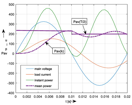
Figure 1. Principal time-waveform of $P_{av}\left(k\right)$ by using of MAF method: step $k=0.5$ ms, length of sliding window $l=T/2=0.01$ s.

The length of the sliding window was taken as T/2, and the number of window points N = 20.

2.2. Using Digital Filtering

The transfer function of a digital filter is formally similar to any system transfer

$$H\left(z\right)=\frac{b_{0-n}.z^{-n}}{a_{0-n}.z^{-n}},$$

(12)

where sequence $f\left\{a_{0-n}\right\}$ represents input signal and $f\left\{b_{0-n}\right\}$ output one. It is, therefore, relatively easy to use a filter to extract the fundamental frequency of real and reactive power components.

Properties of a stable digital filter type of the finite impulse response (DFIR) show its frequency characteristics, in Figure 2.

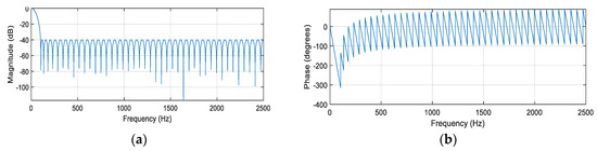
Figure 2. Amplitude—(a) and phase—(b) frequency characteristics of DFIR filter.

Comparison between DFIR and MAF

The frequency characteristics of a moving average filter method (MAF) are shown in Figure 3.

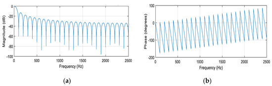
Figure 3. Amplitude—(a) and phase—(b) frequency characteristics of MAF filter.

Using of digital infinite impulse response filter (DIIR) can lead to instability [15,16]. On the other hand, its advantage can be better (faster) attenuation of higher harmonics. Similarly, using the Butterworth filter of 4th order gives good results regarding harmonics attenuation [11]. A comparison of power waveforms worked out by MAF-, DFIR and DIIR filters in the time domain is shown in Figure 4a,b, respectively.

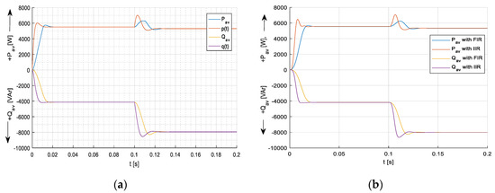
Figure 4. Comparison of power waveforms calculated by different methods MAF and direct function in the time domain $p\left(t\right)$ and $q\left(t\right)$—(a), DFIR and DIIR filters for $P_{av}\left(k\right)$ and $Q_{av}\left(k\right)$ —(b).

The choice of filter is a compromise: the DC term must be passed, and the double frequency term rejected. A sharp, high-order filter will give a long-step response, whereas a low-order filter will give poor separation of the terms and imperfect current cancellation. The resulting system usually has a response time of 2–3 main cycles. So, regarding the speed of calculation and accuracy, we have decided on MAF, although the principal results of both of them are very similar (see Figure 4a,b).

After worked-out the DC power components $P_{av}$ and $Q_{av}$, we can easily calculate AC components $p_{ac}\left(t\right)$ and $q_{ac}\left(t\right)$.

$$p_{ac}\left(t\right)=p\left(t\right)-P_{av}\left(k\right),$$

(13a)

$$q_{ac}\left(t\right)=q\left(t\right)-Q_{av}\left(k\right).$$

(13b)

Now, we can determine all components of power, including the power factor

$$S_{av}\left(k\right)=\frac{3}{2}\left[U_{\alpha ,rms}\left(k\right)I_{\alpha ,rms}\left(k\right)+U_{\beta ,rms}\left(k\right)I_{\beta ,rms}\left(k\right)\right]$$

(14)

$$P_{av}\left(k\right)—\mathrm{by} \mathrm{numerical} \mathrm{integration} \mathrm{of} \mathrm{Equation} \left(10\right) \mathrm{using} \mathrm{MAF}$$

(15)

$$Q_{av}\left(k\right)—\mathrm{by} \mathrm{numerical} \mathrm{integration} \mathrm{of} \mathrm{Equation} \left(11\right) \mathrm{using} \mathrm{MAF}$$

(16)

$$D_{av}\left(k\right)=\sqrt{P^2{}_{ac,rms}\left(k\right)+Q^2{}_{ac,rms}},$$

(17)

where $P_{ac,rms}\left(k\right),Q_{ac,rms}\left(k\right)$ are determined by the integral calculus of $p_{ac}\left(t\right)$ and $q_{ac}\left(t\right)$

$$P_{ac,rms}\left(k\right)=\frac{1}{T}\sqrt{\underset{0}{\overset{T}{{\displaystyle \int }}}{p}^2{}_{ac}\left(t\right)\mathrm{d}t},$$

(18a)

$$Q_{ac,rms}\left(k\right)=\frac{1}{T}\sqrt{\underset{0}{\overset{T}{{\displaystyle \int }}}{q}^2{}_{ac}\left(t\right)\mathrm{d}t}.$$

(18b)

Or we can use classical relation

$$D_{av}\left(k\right)=\sqrt{S^2{}_{av}\left(k\right)-P^2{}_{av}\left(k\right)-Q^2{}_{av}\left(k\right)}$$

(19)

when a moving average method should be applied to provide the results in each computation (integration) step $k$.

The power factor is defined as the relation between $P_{av}$ and $S_{av}$, thus

$$PF\left(k\right)=\frac{P_{av}\left(k\right)}{S_{av}\left(k\right)}.$$

(20)

Regarding total harmonic distortion, it can be calculated by the definition of IEC standards [21] using harmonic analysis or rms values of the sum of higher harmonics $Y_{\mathsf{\Sigma }vrms}$ and total quantity $Y_{rms}$

$$TH{D}_{[\%]}=\frac{\sqrt{{\sum }_{\nu =2}^{\nu =\infty }{Y}^2{}_{\nu rms}}}{\sqrt{{\sum }_{\nu =1}^{\nu =\infty }{Y}^2{}_{\nu rms}}}100\%$$

(21a)

$$\mathrm{that} \mathrm{is} TH{D}_{[\%]}=\frac{Y_{\mathsf{\Sigma }\nu rms}}{Y_{rms}}100\%.$$

(21b)

Another approach uses the Cauchy method of residues [22]; for impulse system quantities using infinite series [23]. Relation (21b) can be adapted for input current (under harmonic voltage). See derivation (32).

$$THD\left(k\right)=\frac{D_{av}\left(k\right)}{S_{av}\left(k\right)}.$$

(22)

The maximal limit for total harmonic distortion for the input voltage is recommended at 5% (by IEEE standard [24]), with the largest single harmonic being no more than 3% of the fundamental voltage.

So, now each power component can be determined in any computation step (k). Further, using Fourier analysis, applied to active $P_{av}\left(k\right)$, or reactive $Q_{av}\left(k\right)$ power components, we obtain the active and reactive power of the fundamental harmonic $P_{1av}\left(k\right)$ and $Q_{1av}\left(k\right)$, and at the same time $\cos {\phi }_1\left(k\right)$-power factor of fundamental and $\sin {\phi }_1\left(k\right)$, respectively.

2.3. Taking the Clarke Transform for a Non-Symmetrical System

Since for non-symmetrical system is valid

$$x_a\left(t\right)+x_b\left(t\right)+x_c\left(t\right)\ne 0,$$

(23)

because of including a zero-phase sequence component $x_0\left(t\right)$ into Clarke transform [1,25,26,27].

$$\left[\begin{array}{c}{x}_{\alpha }\left(t\right)\\ x_{\beta }\left(t\right)\\ x_0\left(t\right)\end{array}\right]=\frac{2}{3}\left[\begin{array}{ccc}1& -\frac{1}{2}& -\frac{1}{2}\\ 0& \frac{\sqrt{3}}{2}& -\frac{\sqrt{3}}{2}\\ \frac{1}{2}& \frac{1}{2}& \frac{1}{2}\end{array}\right]\left[\begin{array}{c}{x}_a\left(t\right)\\ x_b\left(t\right)\\ x_c\left(t\right)\end{array}\right].$$

(24)

The inverse transformation into $a,b,c$-system can be obtained using the inverse transformation matrix. Consequently, the power in a non-symmetrical system also features an instantaneous zero-sequence component $p_0\left(t\right)$.

$$\left[\begin{array}{c}\begin{array}{c}{p}_{\alpha ,\beta }\left(t\right)\\ q_{\alpha ,\beta }\left(t\right)\end{array}\\ p_0\left(t\right)\end{array}\right]=\frac{3}{2}\left[\begin{array}{ccc}{u}_{\alpha }\left(t\right)& u_{\beta }\left(t\right)& 0\\ -u_{\beta }\left(t\right)& u_{\alpha }\left(t\right)& 0\\ 0& 0& \frac{u_0\left(t\right)}{3}\end{array}\right]\left[\begin{array}{c}{i}_{\alpha }\left(t\right)\\ i_{\beta }\left(t\right)\\ i_0\left(t\right)\end{array}\right].$$

(25)

The phase power components $p_{a,b,c}\left(t\right)$ can be expressed by the inverse transform of this Equation (23) or by introducing a new transform [7]; the following equations are obtained

$$\left[\begin{array}{c}\begin{array}{c}{p}_a\left(t\right)\\ p_b\left(t\right)\end{array}\\ p_c\left(t\right)\end{array}\right]=\left[\begin{array}{c}\begin{array}{c}{p}_{ap}\left(t\right)\\ p_{bp}\left(t\right)\end{array}\\ p_{cp}\left(t\right)\end{array}\right]+\left[\begin{array}{c}\begin{array}{c}{p}_{aq}\left(t\right)\\ p_{bq}\left(t\right)\end{array}\\ p_{cq}\left(t\right)\end{array}\right]+\left[\begin{array}{c}\begin{array}{c}{p}_{a0}\left(t\right)\\ p_{b0}\left(t\right)\end{array}\\ p_{c0}\left(t\right)\end{array}\right].$$

(26)

Instantaneous reactive powers in each phase $p_{aq}\left(t\right),p_{bq}\left(t\right),p_{cq}\left(t\right)$ make no contribution to the instantaneous power flow in the three-phase non-symmetrical system. The instantaneous active power flow is represented by the sum of $p_{\alpha ,\beta }\left(t\right)$, and $p_0\left(t\right)$ because the sum of the instantaneous reactive powers $p_{aq}\left(t\right),p_{bq}\left(t\right),p_{cq}\left(t\right)$ is always zero [7].

3. Modelling and Simulation

The simulation was performed in Matlab/Simulink environment. The ‘moving-average function’ and ‘moving-RMS function’ has been used to provide a sliding window for instantaneously AVE and RMS value calculations.

Parameters of the phase voltages in $\alpha , \beta$-system

$$U_{\alpha ,rms}=230 V \gg U_{\alpha ,max}\cong 325 V \gg u_{\alpha }\left(t\right)=U_{\alpha ,max}\sin \left(\omega t\right),$$

(27a)

$$U_{\beta ,rms}=230 V \gg U_{\beta ,max}\cong 325 V \gg u_{\beta }\left(t\right)=-U_{\beta ,max}\cos \left(\omega t\right).$$

(27b)

Parameters of the Load

Considering load power factor $\cos \left(\phi \right)=0.8$ and impedance $23 \mathsf{\Omega }$, the parameters of the load will be $R=18.4 \mathsf{\Omega }$, $\omega L=13.8 \mathsf{\Omega } \gg L=43.93 \mathrm{mH}$ for $f=50 \mathrm{Hz}$, and the phase currents $I_{\alpha ,rms}=10 \mathrm{A}, I_{\beta ,rms}=10 \mathrm{A}$.

Under harmonic supply voltage, the phase current waveforms are:

$$i_{\alpha }\left(t\right)=I_{\alpha ,max}\sin \left(\omega t-\phi \right),i_{\beta }\left(t\right)=-I_{\beta ,max}\cos \left(\omega t-\phi \right)$$

(28)

where $\phi =\mathrm{atan}\left(\omega \tau \right), \tau =L/R$.

In the case of harmonic waveforms of the voltage and current (under linear load):

$$PF=\frac{P_1}{S_1}=\frac{U_{1,rms}{I}_{1,rms}\cos {\phi }_1}{U_{1,rms}·I_{1,rms}}=\cos {\phi }_1.$$

(29)

This means that the power factor is equal to the cosine of the phase shift—the fundamental harmonic factor.

In the case of a harmonic voltage profile and a non-harmonic current profile, the power factor will be:

$$PF=\frac{P_{1,av}}{S_{av}}=\frac{U_{1,rms}\sqrt{{\sum }_{\nu =1}^{\infty }{\left(I_{\nu ,ef}\right)}^2\cos {\phi }_{\nu }}}{U_{1,rms}·I_{rms}}=\frac{I_{1,rms}}{I_{rms}}\cos {\phi }_1$$

(30)

since all products of the higher harmonic components of the current and $U_{1,rms}$ are zero.

Analogically, the total harmonic distortion of the input current can be expressed as

$$TH{D}_{i[\%]}=\frac{I_{\mathsf{\Sigma }\nu rms}}{I_{rms}}\frac{U_{rms}}{U_{rms}}100\%=\frac{D_{av}}{S_{av}}100\%$$

(31)

3.1. Mode #1 Harmonic Supply and Linear R-L Load

There are considered systems when 3-, 5-, and 2-phase networks supply linear RL loads, Figure 5.

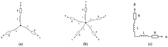
Figure 5. The basic scheme of the considered linear RL load for 3- (a), 5- (b), and 2- (c) phase systems.

3.1.1. 3-Phase Network and Linear Passive RL Load

Parameters for steady states at $t\in ⟨0.0;0.1⟩$ and at $t\in ⟨0.1;0.2⟩$ are given in the Table 1:

Table 1. Load parameters for steady states before and after load change.

Load	$\mathit{R} \left[\mathbf{\Omega }\right]$	$\mathit{L} \left[\mathbf{mH}\right]$	$\mathit{Z} \left[\mathbf{\Omega }\right]$	$\mathit{\tau }$ $\left[\mathbf{ms}\right]$	$\mathit{\phi }$ $[°\mathbf{el}.]$	$\mathbf{cos}\mathit{\phi }[-]$	$\mathbf{sin} \mathit{\phi } [-]$
before	$18.4$	$43.93$	$23$	$2.39$	$36.76$	$0.8$	$0.6$
after	$9.2$	$43.93$	$16.59$	$4.78$	$56.33$	$0.5545$	$0.8322$

$U_{rms}=230 V, f=50 \mathrm{Hz}$, 3-phase system.

Power components average values, classical calculus are shown in Table 2.

Table 2. Classical calculation before and after the change (at steady states).

Time	${\mathit{S}}_{\mathit{a}\mathit{v}}\left[\mathbf{VA}\right]$	${\mathit{P}}_{\mathit{a}\mathit{v}}\left[\mathbf{W}\right]$	${\mathit{Q}}_{\mathit{a}\mathit{v}}\left[\mathbf{VAr}\right]$	${\mathit{D}}_{\mathit{a}\mathit{v}}[\mathbf{VAd}]$	$\mathit{P}\mathit{F}[-]$	${\mathit{A}}_1\left[\mathbf{A}\right]$	$\mathbf{cos} {\mathit{\phi }}_1\left[\mathbf{W}\right]$
$\mathrm{t}=0.1 \mathrm{s}$	$6900$	$5520$	$4140$	$0$	$0.8000$	$14.14$	$0.8000$
$\mathrm{t}=0.2 \mathrm{s}$	$9556.6$	$5305$	$7961$	$0$	$0.5546$	$19.60$	$0.5546$

$U_{\alpha ,rms}=230 \mathrm{V}, U_{\beta ,rms}=230 \mathrm{V},I_{\alpha ,rms}=10 \mathrm{A},I_{\beta ,rms}=10 \mathrm{A},I_{\alpha ,rms}=13.86 \mathrm{A}, I_{\beta ,rms}=13.86 \mathrm{A}$.

Simulation Results, Simulation Step 200 μs

Measurable quantities, i.e., voltages and currents in $\alpha ,\beta \left(rms\right)$, and their parameters are given in Table 3.

Table 3. Simulation results before and after the change (at steady states).

Time	${\mathit{U}}_{\mathit{\alpha },\mathit{r}\mathit{m}\mathit{s}}\left[\mathbf{V}\right]$	${\mathit{U}}_{\mathit{\beta },\mathit{r}\mathit{m}\mathit{s}}\left[\mathbf{V}\right]$	${\mathit{I}}_{\mathit{\alpha },\mathit{r}\mathit{m}\mathit{s}}\left[\mathbf{A}\right]$	${\mathit{I}}_{\mathit{\beta },\mathit{r}\mathit{m}\mathit{s}}\left[\mathbf{A}\right]$	${\mathit{A}}_1 \left[\mathbf{A}\right]$	${\mathit{\phi }}_1\left[°\mathbf{e}\mathbf{l}.\right]$	$\mathbf{cos}{\mathit{\phi }}_1[-]$
t = 0.1 s	229.8	229.8	9.991	9.991	14.13	36.88	0.7947
t = 0.2 s	229.8	229.8	13.85	13.85	19.60	56.31	0.5547

Power component average values, computed in Matlab/Simulink are given in Table 4.

Table 4. Simulation results before and after the change (at steady states).

Time	${\mathit{S}}_{\mathit{a}\mathit{v}}\left[\mathbf{V}\mathbf{A}\right]$	${\mathit{P}}_{\mathit{a}\mathit{v}}\left[\mathbf{W}\right]$	${\mathit{Q}}_{\mathit{a}\mathit{v}}\left[\mathbf{V}\mathbf{A}\mathbf{r}\right]$	${\mathit{D}}_{\mathit{a}\mathit{v}}[\mathbf{V}\mathbf{A}\mathbf{d}]$	$\mathit{P}\mathit{F}[-]$	$\mathit{T}\mathit{H}{\mathit{D}}_{\mathit{i}}[\%]$	${\mathit{P}}_{0\mathit{a}\mathit{v}}\left[\mathbf{W}\right]$
t = 0.1 s	6888.5	5510.6	4133.3	0	0.7999	0	0
t = 0.2 s	9551.5	5298.9	7946.9	0	0.5547	0	0

As can be seen, the calculated and simulated values of power components are nearly the same. Network voltages and currents in $a,b,c$- system during transient, Figure 6.

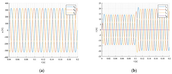
Figure 6. Phase voltages (a), currents (b) in a,b,c—coordinates.

Apparent, active, blind, and distortion powers during transient states are shown, due to comparison to 5- and 2-phase systems, at the end of Section 3.1.

3-Phase Network and Active Load—3-Phase IM Motor

Parameters of the 3-phase 4-pole IM motor at $t\in ⟨0.2;0.4⟩$ and $t\in ⟨0.4;0.6⟩$ are given in Table 5.

Table 5. IM motor parameters for steady-state before and after load change.

Load	${\mathit{T}}_{\mathit{l}}$ $\left[\mathbf{N}\mathbf{m}\right]$	${\mathit{J}}_{\mathit{m}}$ $\left[\mathbf{k}\mathbf{g}{\mathbf{m}}^2\right]$	${\mathit{R}}_{\mathit{s}} \left[\mathbf{\Omega }\right]$	${\mathit{R}}_{\mathit{r}} \left[\mathbf{\Omega }\right]$	${\mathit{L}}_{\mathit{s}} \left[\mathbf{m}\mathbf{H}\right]$	${\mathit{L}}_{\mathit{r}} \left[\mathbf{m}\mathbf{H}\right]$	${\mathit{L}}_{\mathit{m}} \left[\mathbf{H}\right]$
before	$24$	$0.0343$	$0.7384$	$0.7402$	$3.045$	$3.045$	$0.1241$
after	$48$	$0.0343$	$0.7384$	$0.7402$	$3.045$	$3.045$	$0.1241$

$U_{max}=325 \mathrm{V}, Pp=2, f=50 \mathrm{Hz}$.

The torque of the motor $T_l$ has been changed to $2*T_l$ at $t=0.4 \mathrm{s}$.

Simulation Results, Simulation Step 200 μs

Measurable quantities, i.e., voltages and currents in $\alpha ,\beta \left(rms\right)$, and their parameters are given in Table 6.

Table 6. Simulation results before and after the change (at steady states).

Time	${\mathit{U}}_{\mathit{\alpha },\mathit{r}\mathit{m}\mathit{s}} \left[\mathbf{V}\right]$	${\mathit{U}}_{\mathit{\beta },\mathit{r}\mathit{m}\mathit{s}} \left[\mathbf{V}\right]$	${\mathit{I}}_{\mathit{\alpha },\mathit{r}\mathit{m}\mathit{s} }\left[\mathbf{A}\right]$	${\mathit{I}}_{\mathit{\beta },\mathit{r}\mathit{m}\mathit{s}} \left[\mathbf{A}\right]$	${\mathit{A}}_1 \left[\mathbf{A}\right]$	${\mathit{\phi }}_1 \left[°\mathbf{e}\mathbf{l}.\right]$	$\mathbf{c}\mathbf{o}\mathbf{s}{\mathbf{\phi }}_1 [-]$
$\mathrm{t}=0.4 \mathrm{s}$	$229.8$	$229.8$	8.145	8.148	11.52	45.66	0.70
$\mathrm{t}=0.6 \mathrm{s}$	$229.8$	$229.8$	13.21	13.22	18.69	29.30	0.87

Corresponding power component average values, computed in Matlab/Simulink are given in Table 7.

Table 7. Simulation results before and after the change (at steady states).

Time	${\mathit{S}}_{\mathit{a}\mathit{v}} \left[\mathit{k}\mathbf{V}\mathbf{A}\right]$	${\mathit{P}}_{\mathit{a}\mathit{v}} \left[\mathit{k}\mathbf{W}\right]$	${\mathit{Q}}_{\mathit{a}\mathit{v}} \left[\mathit{k}\mathbf{V}\mathbf{A}\mathbf{r}\right]$	${\mathit{D}}_{\mathit{a}\mathit{v}} [\mathbf{V}\mathbf{A}\mathbf{d}]$	$\mathit{P}\mathit{F} [-]$	$\mathit{T}\mathit{H}{\mathit{D}}_{\mathit{i}}[\%]$	${\mathit{P}}_{1\mathit{a}\mathit{v}} \left[\mathbf{W}\right]$	${\mathit{P}}_{0\mathit{a}\mathit{v}} \left[\mathbf{W}\right]$
$\mathrm{t}=0.4 \mathrm{s}$	5.616	3.932	4.010	4.566	0.70	$0.08$	3.932	$0$
$\mathrm{t}=0.6 \mathrm{s}$	9.109	7.937	4.459	12.27	0.87	$0.135$	7.936	$0$

Network voltages are the same as in the previous case. Phase currents in a,b,c- system during transient are shown in Figure 7a. Electromagnetic quantities, namely torque and angular speed, are given in Figure 7b.

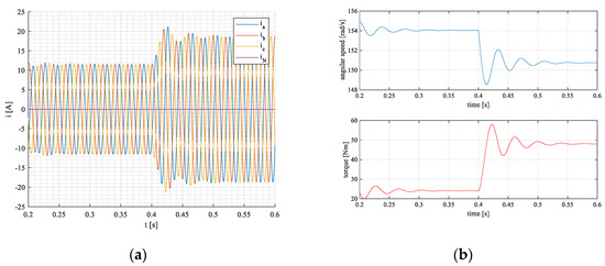
Figure 7. Phase voltages (a), currents (b) in a,b,c—coordinates.

Apparent, active, blind, and distortion powers during the transient state are in Figure 8a–d.

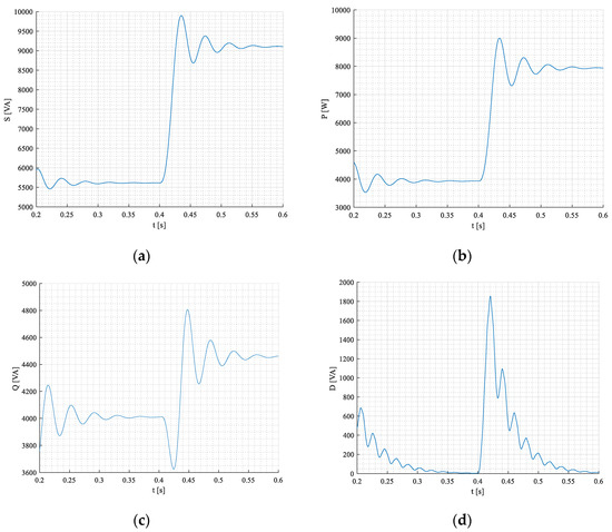
Figure 8. Apparent—(a), active—(b), blind—(c), and distortion (d) power components during transient states of induction motor.

3.1.2. 5-Phase Network and Linear RL Load

Parameters for steady states at $t\in ⟨0.0;0.1⟩$ and at $t\in ⟨0.1;0.2⟩$ are given in the Table 8:

Table 8. Load parameters for steady states before and after load change.

Load	$\mathit{R} \left[\mathbf{\Omega }\right]$	$\mathit{L} \left[\mathbf{m}\mathbf{H}\right]$	$\mathit{Z} \left[\mathbf{\Omega }\right]$	$\mathit{\tau } \left[\mathbf{m}\mathbf{s}\right]$$$	$\mathit{\phi }$$[°\mathbf{e}\mathbf{l}.]$	$\mathbf{c}\mathbf{o}\mathbf{s} \mathit{\phi }[-]$$$	$\mathbf{s}\mathbf{i}\mathbf{n} \mathit{\phi } [-]$
before	$18.4$	$43.93$	$23$	$2.39$	$36.76$	$0.8$	$0.6$
after	$9.2$	$43.93$	$16.59$	$4.78$	$56.33$	$0.5545$	$0.8322$

$U_{rms}=230 \mathrm{V}, f=50 \mathrm{Hz}$, 5-phase system.

Power components average values, classical calculus are shown in a Table 9.

Table 9. Classical calculation before and after the change (at steady states).

Time	${\mathit{S}}_{\mathit{a}\mathit{v}} \left[\mathbf{V}\mathbf{A}\right]$	${\mathit{P}}_{\mathit{a}\mathit{v}} \left[\mathbf{W}\right]$	${\mathit{Q}}_{\mathit{a}\mathit{v}} \left[\mathbf{V}\mathbf{A}\mathbf{r}\right]$	${\mathit{D}}_{\mathit{a}\mathit{v}} [\mathbf{V}\mathbf{A}\mathbf{d}]$	$\mathit{P}\mathit{F} \left[–\right]$	${\mathit{A}}_1 \left[\mathbf{A}\right]$	$\mathbf{c}\mathbf{o}\mathbf{s} {\mathit{\phi }}_1 \left[\mathbf{W}\right]$
$\mathrm{t}=0.1 \mathrm{s}$	$11,500$	$9200$	$6900$	$0$	$0.8000$	$14.14$	$0.8000$
$\mathrm{t}=0.2 \mathrm{s}$	$15,927$	$8842$	$13,268$	$0$	$0.5546$	$19.60$	$0.5546$

$U_{\alpha ,rms}=230 \mathrm{V}, U_{\beta ,rms}=230 \mathrm{V}, I_{\alpha ,rms}=10 \mathrm{A}, I_{\beta ,rms}=10 \mathrm{A}, I_{\alpha ,rms}=13.86 \mathrm{A}, I_{\beta ,rms}=13.86 \mathrm{A}$.

Simulation Results, Simulation Step 200 μs

Measurable quantities i.e., voltages and currents in $\alpha ,\beta \left(rms\right)$, and their parameters are given in Table 10.

Table 10. Simulation results before and after the change (at steady states).

Time	${\mathit{U}}_{\mathit{\alpha },\mathit{r}\mathit{m}\mathit{s}} \left[\mathbf{V}\right]$	${\mathit{U}}_{\mathit{\beta },\mathit{r}\mathit{m}\mathit{s}} \left[\mathbf{V}\right]$	${\mathit{I}}_{\mathit{\alpha },\mathit{r}\mathit{m}\mathit{s}} \left[\mathbf{A}\right]$	${\mathit{I}}_{\mathit{\beta },\mathit{r}\mathit{m}\mathit{s}} \left[\mathbf{A}\right]$	${\mathit{A}}_1 \left[\mathbf{A}\right]$	${\mathit{\phi }}_1 \left[°\mathbf{e}\mathbf{l}.\right]$	$\mathbf{c}\mathbf{o}\mathbf{s} {\mathbf{\phi }}_1 [-]$
$\mathrm{t}=0.1 \mathrm{s}$	$229.8$	$229.8$	$9.991$	$9.991$	$14.13$	$36.88$	$0.7947$
$\mathrm{t}=0.2 \mathrm{s}$	$229.8$	$229.8$	$13.85$	$13.85$	$19.60$	$56.31$	$0.5547$

Power component average values, computed in Matlab/Simulink are given in Table 11.

Table 11. Simulation results before and after the change (at steady states).

Time	${\mathit{S}}_{\mathit{a}\mathit{v}} \left[\mathbf{V}\mathbf{A}\right]$	${\mathit{P}}_{\mathit{a}\mathit{v}} \left[\mathbf{W}\right]$	${\mathit{Q}}_{\mathit{a}\mathit{v}} \left[\mathbf{V}\mathbf{A}\mathbf{r}\right]$	${\mathit{D}}_{\mathit{a}\mathit{v}} [\mathbf{V}\mathbf{A}\mathbf{d}]$	$\mathit{P}\mathit{F} [-]$	$\mathit{T}\mathit{H}{\mathit{D}}_{\mathit{i}} [\mathit{\%}]$	${\mathit{P}}_{1\mathit{a}\mathit{v}} \left[\mathbf{A}\right]$	${\mathit{P}}_{0\mathit{a}\mathit{v}} \left[\mathbf{W}\right]$
$\mathrm{t}=0.1 \mathrm{s}$	$11,479.8$	$9182.8$	$6689.3$	$0$	$0.7999$	$0.0$	$9123.2$	$0$
$\mathrm{t}=0.2 \mathrm{s}$	$15,916.7$	$8828.7$	$13,243.7$	$0$	$0.5547$	$0.0$	$8833.2$	$0$

As can be seen, the calculated and simulated values of power components are nearly the same. Network voltages and currents in $a,b,c$- system during transient, Figure 9a,b.

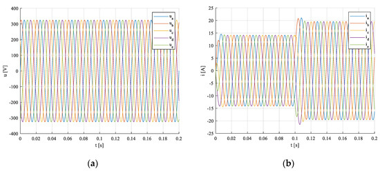
Figure 9. Phase voltages (a) and currents (b) in $a,b,c,d,e$—coordinates.

Apparent, active, blind, and distortion powers during transient states are shown, due to comparison to 5- and 2-phase systems, in Figure 11a–d.

3.1.3. 2-Phase Network and Linear RL Load

Parameters for steady states at $t\in ⟨0.0;0.1⟩$ and at $t\in ⟨0.1;0.2⟩$ are given in the Table 12:

Table 12. Load parameters for steady states before and after load change.

Load	$\mathit{R} \left[\mathbf{\Omega }\right]$	$\mathit{L} \left[\mathbf{m}\mathbf{H}\right]$	$\mathit{Z} \left[\mathbf{\Omega }\right]$	$\mathit{\tau }$$\left[\mathbf{m}\mathbf{s}\right]$	$\mathit{\phi }$$[°\mathbf{e}\mathbf{l}.]$	$\mathbf{c}\mathbf{o}\mathbf{s} \mathit{\phi }$$[-]$	$\mathbf{s}\mathbf{i}\mathbf{n} \mathit{\phi } [-]$
before	$18.4$	$43.93$	$23$	$2.39$	$36.76$	$0.8$	$0.6$
after	$9.2$	$43.93$	$16.59$	$4.78$	$56.33$	$0.5545$	$0.8322$

$U_{rms}=230 \mathrm{V}, f=50 \mathrm{Hz}$, 2-phase system.

Power components average values, classical calculus, given in Table 13:

Table 13. Classical calculation before and after the change (at steady states).

Time	${\mathit{S}}_{\mathit{a}\mathit{v}} \left[\mathbf{V}\mathbf{A}\right]$	${\mathit{P}}_{\mathit{a}\mathit{v}} \left[\mathbf{W}\right]$	${\mathit{Q}}_{\mathit{a}\mathit{v}} \left[\mathbf{V}\mathbf{A}\mathbf{r}\right]$	${\mathit{D}}_{\mathit{a}\mathit{v}} [\mathbf{V}\mathbf{A}\mathbf{d}]$	$\mathit{P}\mathit{F} [-]$	${\mathit{A}}_1 \left[\mathbf{A}\right]$	$\mathbf{cos} {\mathit{\phi }}_1 \left[\mathbf{W}\right]$
$\mathrm{t}=0.1 \mathrm{s}$	$4600$	$3680$	$2760$	$0$	$0.8000$	$14.14$	$0.8000$
$\mathrm{t}=0.2 \mathrm{s}$	$6371$	$3537$	$5307$	$0$	$0.5546$	$19.60$	$0.5546$

$U_{\alpha ,rms}=230 \mathrm{V}, U_{\beta ,rms}=230 \mathrm{V}, I_{\alpha ,rms}=10 \mathrm{A}, I_{\beta ,rms}=10 \mathrm{A}, I_{\alpha ,rms}=13.86 \mathrm{A}, I_{\beta ,rms}=13.86 \mathrm{A}$.

Simulation Results, Simulation Step 200 μs

Measurable quantities, i.e., voltages and currents in $\alpha ,\beta \left(rms\right)$, and their parameters are given in Table 14.

Table 14. Simulation results before and after the change (at steady states).

Time	${\mathit{U}}_{\mathit{\alpha },\mathit{r}\mathit{m}\mathit{s}} \left[\mathbf{V}\right]$	${\mathit{U}}_{\mathit{\beta },\mathit{r}\mathit{m}\mathit{s}} \left[\mathbf{V}\right]$	${\mathit{I}}_{\mathit{\alpha },\mathit{r}\mathit{m}\mathit{s}} \left[\mathbf{A}\right]$	${\mathit{I}}_{\mathit{\beta },\mathit{r}\mathit{m}\mathit{s}} \left[\mathbf{A}\right]$	${\mathit{A}}_1 \left[\mathbf{A}\right]$	${\mathit{\phi }}_1 \left[°\mathbf{el}.\right]$	$\mathbf{c}\mathbf{o}\mathbf{s} {\mathit{\phi }}_1 [-]$
$\mathrm{t}=0.1 \mathrm{s}$	$229.8$	$229.8$	$9.991$	$9.991$	$14.13$	$36.88$	$0.7947$
$\mathrm{t}=0.2 \mathrm{s}$	$229.8$	$229.8$	$13.85$	$13.85$	$19.60$	$56.31$	$0.5547$

Power component average values, computed in Matlab/Simulink are given in Table 15.

Table 15. Simulation results before and after the change (at steady states).

Time	${\mathit{S}}_{\mathit{a}\mathit{v}} \left[\mathbf{VA}\right]$	${\mathit{P}}_{\mathit{a}\mathit{v}} \left[\mathbf{W}\right]$	${\mathit{Q}}_{\mathit{a}\mathit{v}} \left[\mathbf{VAr}\right]$	${\mathit{D}}_{\mathit{a}\mathit{v}} [\mathbf{VAd}]$	$\mathit{P}\mathit{F} [-]$	$\mathit{T}\mathit{H}{\mathit{D}}_{\mathit{i}} [\%]$	${\mathit{P}}_{1\mathit{a}\mathit{v}} \left[\mathbf{W}\right]$	${\mathit{P}}_{0\mathit{a}\mathit{v}} \left[\mathbf{W}\right]$
$\mathrm{t}=0.1 \mathrm{s}$	$4591.9$	$3673.1$	$2755.7$	$0$	$0.7999$	$0.0$	$3649.3$	$0$
$\mathrm{t}=0.2 \mathrm{s}$	$6366.7$	$3531.5$	$5297.5$	$0$	$0.5547$	$0.0$	$3533.3$	$0$

As can be seen, the calculated and simulated values of power components are nearly the same. Network voltages and currents in $a,b$ ($\alpha ,\beta$)- coordinates during transient, Figure 10a,b.

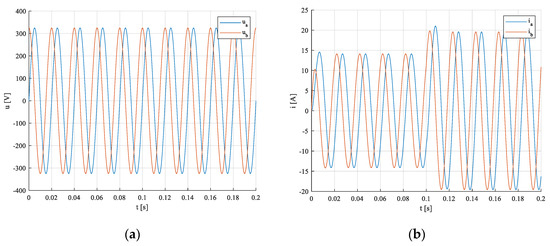
Figure 10. Phase voltages (a) and load currents (b) in $\alpha ,\beta$ coordinates.

3.1.4. Comparison of Power Components in 2-,3- and 5-Phase Supply Systems under RL Load

Apparent, active, blind, and distortion power components during the transient state for 3-, 5-, and 2-phase systems are presented in Figure 11a–d.

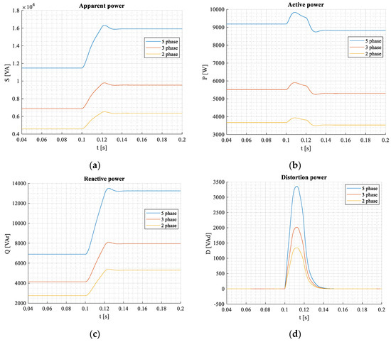
Figure 11. Apparent (a), active (b), blind (c), and distortion (d) power components during transient states for 3-, 5-, and 2-phase systems under mains supplied linear RL load.

The simulation was performed under the same load phase parameters; therefore, the magnitudes are proportionately different.

The waveforms of all power components per unit are very similar, but the interesting is that during the transient response, also a power distortion component is generated, Figure 11d. It is due to different arises of active and reactive (blind) power components (Figure 11b,c). Thus, during the transient state (approx. 3–4-time constants), the spectral density comprises different higher harmonics, which could cause an additional negative influence on the system.

The distortion power calculated by three different methods (MAF, DFIR, and DIIR) for a 3-phase system is presented in Figure 12a. The time dependency of the corresponding current $I_{d,rms}$ for the 3-phase system is shown in Figure 12b.

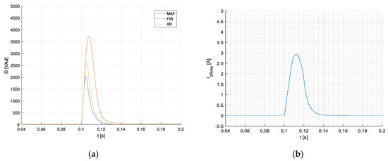
Figure 12. Waveforms of distortion power components $D_{av}\left(k\right)$ during transient states calculated by different methods (MAF-, DFIR, and DIIR filters) (a), and the corresponding deformation component of the current using the MAF method (b).

In this simply case-harmonic supply, linear load—we can verify a time course I_DRms during transient using another method than p-q one. By decomposition of fundamental harmonic current into active and reactive (blind) components, we can calculate the RMS values of these currents. Knowing the RMS value of total harmonic fundamental, the RMS deformation component of the current can be determined as well as in transient states.

So, knowing $P_{av}\left(k\right)$ and $Q_{av}\left(k\right)$ we get

$$\left[\begin{array}{c}{i}_{\alpha }\left(k\right)\\ i_{\beta }\left(k\right)\end{array}\right]=\frac{2}{3}\frac{1}{D}\left[\begin{array}{cc}{u}_{\alpha }\left(k\right)& -u_{\beta }\left(k\right)\\ u_{\beta }\left(k\right)& u_{\alpha }\left(k\right)\end{array}\right]\left[\begin{array}{cc}{P}_{av}\left(k\right)& p_{ac}\left(k\right)\\ Q_{av}\left(k\right)& q_{ac}\left(k\right)\end{array}\right]$$

(32)

where $p_{ac}\left(k\right)$ and $q_{ac}\left(k\right)$ are calculated as (13ab) using the moving average method. Actually, the term $P_{av}\left(k\right)-P_{1av}\left(k\right)$ is zero (also $p_{ac}\left(k\right)$ and $q_{ac}\left(k\right)$) but sometimes, when higher harmonics have to be taken into account, it is not zero. Those $i_{\alpha }\left(k\right)$ and $i_{\beta }\left(k\right)$ currents are simultaneously the reference currents for the active power filter (PAF compensator).

$${\left[\begin{array}{c}{i}_{\alpha }\left(k\right)\\ i_{\beta }\left(k\right)\end{array}\right]}_{ref}=\frac{2}{3}\frac{1}{D}\left[\begin{array}{cc}{u}_{\alpha }\left(k\right)& -u_{\beta }\left(k\right)\\ u_{\beta }\left(k\right)& u_{\alpha }\left(k\right)\end{array}\right]\left[\begin{array}{cc}{P}_{av}\left(k\right)-P_{1av}\left(k\right)& p_{ac}\left(k\right)\\ Q_{av}\left(k\right)& q_{ac}\left(k\right)\end{array}\right].$$

(33)

Before this, they should be back-transformed into $a, b, c,\left(d, e\right)$-phase system.

3.2. Mode #2 Harmonic Supply and Nonlinear Load

Let´s consider systems supplied from a harmonic network and equipped with 3-, 5-, and 2-phase diode rectifiers with a capacitive filter and linear resistive R load, Figure 13a–c.

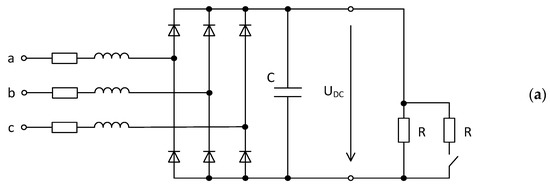
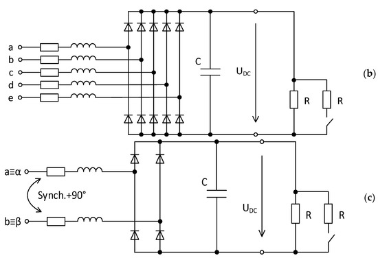
Figure 13. The basic scheme of the considered systems: 3-phase (a), 5-phase (b), and 2-phase (c).

3.2.1. 3-Phase Rectifier with Voltage Output

Parameters for steady states at $t\in ⟨0.0;0.1⟩$ and at $t\in ⟨0.1;0.2⟩$ are given in the Table 16.

Table 16. Load parameters for steady states before and after load change.

Load	$\mathit{R} \left[\mathbf{\Omega }\right]$	$\mathit{C} \left[\mathbf{m}\mathbf{F}\right]$
before	$55.90$	$1.88$
after	$27.95$	$1.88$

$U_{rms}=230 \mathrm{V}, f=50 \mathrm{Hz}$, 3-phase supply system.

Simulation Results, Simulation Step 200 µs

Measurable quantities, i.e., voltages and currents in $\alpha ,\beta \left(rms\right),$ and their parameters are given in Table 17.

Table 17. Simulation results before and after the change (at steady states).

Time	${\mathit{U}}_{\mathit{\alpha },\mathit{r}\mathit{m}\mathit{s}} \left[\mathbf{V}\right]$	${\mathit{U}}_{\mathit{\beta },\mathit{r}\mathit{m}\mathit{s}} \left[\mathbf{V}\right]$	${\mathit{I}}_{\mathit{\alpha },\mathit{r}\mathit{m}\mathit{s}} \left[\mathbf{A}\right]$	${\mathit{I}}_{\mathit{\beta },\mathit{r}\mathit{m}\mathit{s}} \left[\mathbf{A}\right]$	${\mathit{A}}_1 \left[\mathbf{A}\right]$	${\mathit{\phi }}_1 \left[°\mathbf{e}\mathbf{l}.\right]$	$\mathbf{c}\mathbf{o}\mathbf{s} {\mathit{\phi }}_1 [-]$
$\mathrm{t}=0.1 \mathrm{s}$	$229.8$	$229.8$	$19.04$	$19.12$	$11.68$	$-8.045$	$0.9989$
$\mathrm{t}=0.2 \mathrm{s}$	$229.8$	$229.8$	$31.80$	$30.62$	$22.69$	$-10.11$	$0.9924$

Power component average values, computed in Matlab/Simulink are given in Table 18.

Table 18. Simulation results before and after the change (at steady states).

Time	${\mathit{S}}_{\mathit{a}\mathit{v}} \left[\mathbf{VA}\right]$	${\mathit{P}}_{\mathit{a}\mathit{v}} \left[\mathbf{W}\right]$	${\mathit{Q}}_{\mathit{a}\mathit{v}} [\mathbf{VAr}]$	${\mathit{D}}_{\mathit{a}\mathit{v}} [\mathbf{VAd}]$	$\mathit{P}\mathit{F} [-]$	$\mathit{T}\mathit{H}{\mathit{D}}_{\mathit{i}} [\%]$	${\mathit{P}}_{1\mathit{a}\mathit{v}} \left[\mathbf{W}\right]$	${\mathit{P}}_{0\mathit{a}\mathit{v}} \left[\mathbf{W}\right]$
$\mathrm{t}=0.1 \mathrm{s}$	$13,127$	$5535$	$-785.4$	$11,870$	$0.4211$	$90.42$	$5473.9$	$0$
$\mathrm{t}=0.2 \mathrm{s}$	$21,474$	$10,830$	$-1041$	$18,930$	$0.4973$	$88.15$	$10,817.9$	$0$

Network voltages and currents in $a,b,c$- coordinate systems at steady-states are in Figure 14a,b similar to Mode#1.

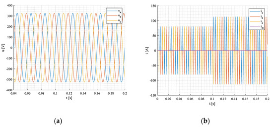
Figure 14. Network voltages (a) and currents (b) in $a,b,c$- coordinate systems.

Voltage (a) and current (b) on the DC side of the rectifier, under step change of resistive load, are shown in Figure 15a,b.

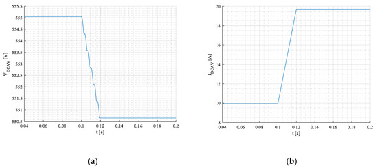
Figure 15. Voltage (a) and current (b) on the DC side of a rectifier, under step change of resistive load.

Apparent, active, blind, and distorted power components during the transient state are shown at the end of the Section 3.2.

3.2.2. 5-Phase Rectifier with Voltage Output

Parameters for steady states at $t\in ⟨0.0;0.1⟩$ and at $t\in ⟨0.1;0.2⟩$ are given in the Table 19.

Table 19. Load parameters for steady states before and after load change.

Load	$\mathit{R} \left[\mathsf{\Omega }\right]$	$\mathit{C} \left[\mathbf{mF}\right]$
before	$55.90$	$1.88$
after	$27.95$	$1.88$

$U_{rms}=230 \mathrm{V}, f=50 \mathrm{Hz}$, 5-phase supply system.

Simulation Results, Simulation Step 200 µs

Measurable quantities, i.e., voltages and currents in $\alpha ,\beta \left(rms\right)$, and their parameters are given in Table 20.

Table 20. Simulation results before and after the change (at steady states).

Time	${\mathit{U}}_{\mathit{\alpha },\mathit{r}\mathit{m}\mathit{s}} \left[\mathbf{V}\right]$	${\mathit{U}}_{\mathit{\beta },\mathit{r}\mathit{m}\mathit{s}} \left[\mathbf{V}\right]$	${\mathit{I}}_{\mathit{\alpha },\mathit{r}\mathit{m}\mathit{s}} \left[\mathbf{A}\right]$	${\mathit{I}}_{\mathit{\beta },\mathit{r}\mathit{m}\mathit{s}} \left[\mathbf{A}\right]$	${\mathit{A}}_1 \left[\mathbf{A}\right]$	${\mathit{\phi }}_1 \left[°\mathbf{el}.\right]$	$\mathbf{cos} {\mathit{\phi }}_1 \left[-\right]$
$\mathrm{t}=0.1 \mathrm{s}$	$229.8$	$229.8$	$12.17$	$12.17$	$8.352$	$-5.988$	$0.9945$
$\mathrm{t}=0.2 \mathrm{s}$	$229.8$	$229.8$	$20.42$	$20.42$	$16.60$	$-7.137$	$0.9923$

Power component average values, computed in Matlab/Simulink are given in Table 21.

Table 21. Simulation results before and after the change (at steady states).

Time	${\mathit{S}}_{\mathit{a}\mathit{v}} \left[\mathbf{VA}\right]$	${\mathit{P}}_{\mathit{a}\mathit{v}} \left[\mathbf{W}\right]$	${\mathit{Q}}_{\mathit{a}\mathit{v}} \left[\mathbf{VAr}\right]$	${\mathit{D}}_{\mathit{a}\mathit{v}} [\mathbf{VAd}]$	$\mathit{P}\mathit{F} [-]$	$\mathit{T}\mathit{H}{\mathit{D}}_{\mathit{i}} [\%]$	${\mathit{P}}_{1\mathit{a}\mathit{v}} \left[\mathbf{W}\right]$	${\mathit{P}}_{0\mathit{a}\mathit{v}} \left[\mathbf{W}\right]$
$\mathrm{t}=0.1 \mathrm{s}$	$13,247.7$	$6359.6$	$-621.7$	$11,667.4$	$0.4797$	$88.07$	$6348.4$	$0$
$\mathrm{t}=0.2 \mathrm{s}$	$24,278.7$	$13,887.3$	$-1798.8$	$9833.4$	$0.5719$	$40.50$	$13,383.1$	$0$

Network voltages and currents in $a,b,c,d,e$- coordinate system at steady-states are given in Figure 16a,b similar to those in Mode#1.

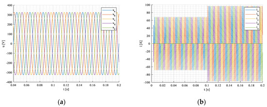
Figure 16. Phase voltages (a), currents (b) in $a,b,c,d,e$- coordinate system during transient.

Voltage and current on the DC side of the rectifier under step change of resistive load are shown in Figure 17a,b.

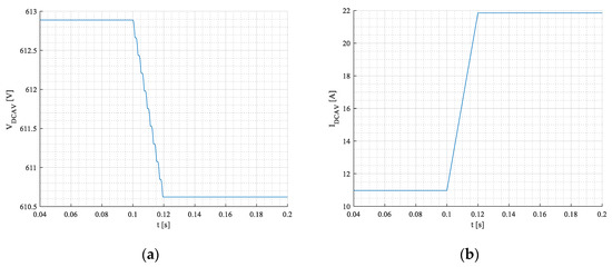
Figure 17. Voltage (a) and current (b) in the DC side under step change of resistive load.

Apparent, active, blind, and distortion powers during transient states are shown in Figure 20a–d.

3.2.3. 2-Phase Rectifier with Voltage Output

Parameters for steady states at $t\in ⟨0.0;0.1⟩$ and at $t\in ⟨0.1;0.2⟩$ are given in the Table 22.

Table 22. Load parameters for steady states before and after load change.

Load	$\mathit{R} \left[\mathsf{\Omega }\right]$	$\mathit{C} \left[\mathbf{mF}\right]$
before	$55.90$	$1.88$
after	$27.95$	$1.88$

$U_{rms}=230 \mathrm{V}, f=50 \mathrm{Hz}$, 2-phase supply system.

Simulation Results, Simulation Step 200 µs

Measurable quantities, i.e., voltages and currents in $\alpha ,\beta \left(rms\right)$, and their parameters are given in Table 23.

Table 23. Simulation results before and after the change (at steady states).

Time	${\mathit{U}}_{\mathit{\alpha },\mathit{r}\mathit{m}\mathit{s}} \left[\mathbf{V}\right]$	${\mathit{U}}_{\mathit{\beta },\mathit{r}\mathit{m}\mathit{s}} \left[\mathbf{V}\right]$	${\mathit{I}}_{\mathit{\alpha },\mathit{r}\mathit{m}\mathit{s}} \left[\mathbf{A}\right]$	${\mathit{I}}_{\mathit{\beta },\mathit{r}\mathit{m}\mathit{s}} \left[\mathbf{A}\right]$	${\mathit{A}}_1 \left[\mathbf{A}\right]$	${\mathit{\phi }}_1 \left[°\mathbf{el}.\right]$	$\mathbf{c}\mathbf{o}\mathbf{s} {\mathit{\phi }}_1 [-]$
$\mathrm{t}=0.1 \mathrm{s}$	$229.8$	$229.8$	$24.47$	$24.47$	$11.17$	$14.19$	$0.9695$
$\mathrm{t}=0.2 \mathrm{s}$	$229.8$	$229.8$	$39.93$	$39.93$	$21.36$	$19.50$	$0.9426$

Power component average values, computed in Matlab/Simulink are given in Table 24.

Table 24. Simulation results before and after the change (at steady states).

Time	${\mathit{S}}_{\mathit{a}\mathit{v}} \left[\mathbf{VA}\right]$	${\mathit{P}}_{\mathit{a}\mathit{v}} \left[\mathbf{W}\right]$	${\mathit{Q}}_{\mathit{a}\mathit{v}} \left[\mathbf{VAr}\right]$	${\mathit{D}}_{\mathit{a}\mathit{v}} [\mathbf{VAd}]$	$\mathit{P}\mathit{F} [-]$	$\mathit{T}\mathit{H}{\mathit{D}}_{\mathit{i}} [\%]$	${\mathit{P}}_{1\mathit{a}\mathit{v}} \left[\mathbf{W}\right]$	${\mathit{P}}_{0\mathit{a}\mathit{v}} \left[\mathbf{W}\right]$
$\mathrm{t}=0.1 \mathrm{s}$	$7934$	$3489$	$-580.9$	$7 034$	$0.4398$	$88.66$	$3484$	$0$
$\mathrm{t}=0.2 \mathrm{s}$	$12,960$	$6548$	$-2182$	$10,722$	$0.5051$	$82.73$	$6546$	$0$

Network voltages and currents in $a,b$- coordinate systems at steady-states are in Figure 18a,b similar to those in Mode#1.

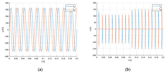
Figure 18. Phase voltages (a), currents in $\alpha ,\beta$ (b) during transient.

Voltage and current on the DC side under step change of resistive load are shown in Figure 19a,b.

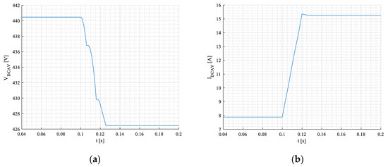
Figure 19. Voltage (a) and current (b) on the DC side under resistive load.

3.2.4. Comparison of Power Components in 2-,3- and 5-Phase Supply Systems under Rectifier Load

Apparent, active, blind, and distortion powers during transient states are shown in Figure 20a–d.

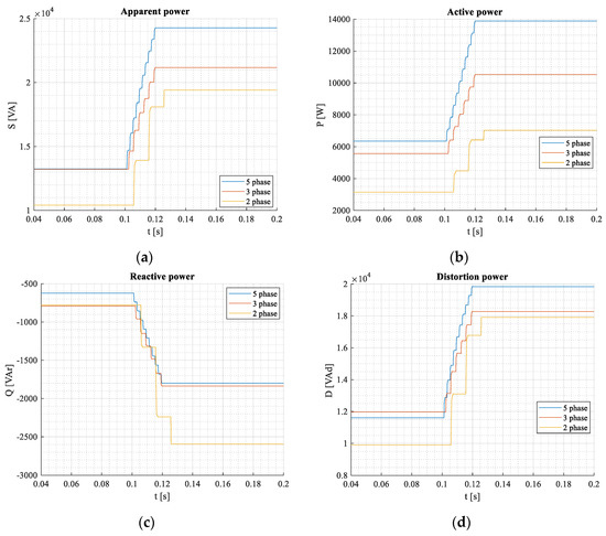
Figure 20. Apparent—(a), active—(b), blind—(c), and distortion (d) power components during transient states for 3-, 5-, and 2-phase systems under mains supplied rectifier load.

The simulation was performed under the same load phase parameters (R, C); therefore, the magnitudes are proportionately different.

The waveforms of all power components per unit are very similar to those in the previous case, Mode#1. In the case of the reactive power component (Figure 20c), nearly the same blind reactive powers of 3- and 5-phase systems are generated at steady-state $t\in ⟨0.1;0.2⟩$ despite DC powers being different. This is mainly due to the fact that the line-to-line voltages of a 5-phase system are not equal to √3 x U_a,b,c as in a 3-phase one, but they are lower. Moreover, the distortion power of a 3-phase system is slightly higher than in a 5-phase one (Figure 20d, $t\in ⟨0.04;0.1⟩$). Distortion components of all connections are rather high due to impulse current taken from the network. Therefore, the power factors are also rather poor.

The reference currents $i_{\alpha ref}\left(k\right)$ and $i_{\beta ref}\left(k\right)$ currents for compensating by power active filter (PAF compensator) are calculated using Equation (27a,b). Before this, they should be back-transformed into $a, b, c$-phase system.

3.3. Mode #3 Non-Harmonic Supply and Linear R-L Load

Now, let´s consider systems consisting of 3-, 5-, and 2-phase VSI inverters with PWM, supplying linear RL load, Figure 21a–c.

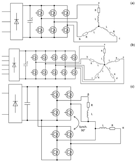
Figure 21. The basic scheme of the considered systems: 3-phase (a), 5-phase (b), and 2-phase (c).

3.3.1. 3-Phase Inverter Type of VSI with Linear RL Load

Parameters for steady states at $t\in ⟨0.0;0.1⟩$ and at $t\in ⟨0.1;0.2⟩$ are given in the Table 25:

Table 25. Load parameters for steady states before and after load change.

Load	$\mathit{R} \left[\mathsf{\Omega }\right]$	$\mathit{L} \left[\mathbf{mH}\right]$	$\mathit{Z} \left[\mathsf{\Omega }\right]$	$\mathit{\tau }$$\left[\mathbf{ms}\right]$	$\mathit{\phi }$ $[\mathbf{el}.]$	$\mathbf{c}\mathbf{o}\mathbf{s} \mathit{\phi }$$[-]$	$\mathbf{s}\mathbf{i}\mathbf{n} \mathit{\phi } [-]$
before	$18.4$	$43.93$	$23$	$2.39$	$36.76$	$0.8$	$0.6$
after	$9.2$	$43.93$	$16.59$	$4.78$	$56.33$	$0.5545$	$0.8322$

$U_{rms}=230 \mathrm{V}, f=50 \mathrm{Hz}$, 3-phase system.

Power components average values, classical calculus, assuming harmonic currents, are given in Table 26:

Table 26. Classical calculation before and after the change (at steady states).

Time	${\mathit{S}}_{1\mathit{a}\mathit{v}} \left[\mathbf{VA}\right]$	${\mathit{P}}_{1\mathit{a}\mathit{v}} \left[\mathbf{W}\right]$	${\mathit{Q}}_{1\mathit{a}\mathit{v}} \left[\mathbf{VAr}\right]$	${\mathit{D}}_{\mathit{a}\mathit{v}} [\mathbf{VAd}]$	$\mathit{P}\mathit{F} [-]$	${\mathit{A}}_1 \left[\mathbf{A}\right]$	$\mathbf{c}\mathbf{o}\mathbf{s} {\mathit{\phi }}_1 \left[\mathbf{W}\right]$
$\mathrm{t}=0.1 \mathrm{s}$	$5070$	$4056$	$3042$	$-$	$-$	$12.12$	$0.8000$
$\mathrm{t}=0.2 \mathrm{s}$	$7028$	$5622$	$4217$	$-$	$-$	$19.60$	$0.5546$

$U_{1\alpha ,rms}=197.2 \mathrm{V}, U_{\beta ,rms}=197.2 \mathrm{V}, I_{\alpha ,rms}=8.57 \mathrm{A}, I_{\beta ,rms}=8.57 \mathrm{A}, I_{\alpha ,rms}=11.88 \mathrm{A}, I_{\beta ,rms}=11.88 \mathrm{A}$.

Simulation Results, Simulation Step 200 µs

Measurable quantities, i.e., voltages and currents in $\alpha ,\beta \left(rms\right)$, and their parameters are given in Table 27.

Table 27. Simulation results before and after the change (at steady states).

Time	${\mathit{U}}_{\mathit{\alpha },\mathit{r}\mathit{m}\mathit{s}} \left[\mathbf{V}\right]$	${\mathit{U}}_{\mathit{\beta },\mathit{r}\mathit{m}\mathit{s}} \left[\mathbf{V}\right]$	${\mathit{I}}_{\mathit{\alpha },\mathit{r}\mathit{m}\mathit{s}} \left[\mathbf{A}\right]$	${\mathit{I}}_{\mathit{\beta },\mathit{r}\mathit{m}\mathit{s}} \left[\mathbf{A}\right]$	${\mathit{A}}_1 \left[\mathbf{A}\right]$	${\mathit{\phi }}_1 \left[°\mathbf{el}.\right]$	$\mathbf{c}\mathbf{o}\mathbf{s} {\mathit{\phi }}_1 [-]$
$\mathrm{t}=0.1 \mathrm{s}$	$238.9$	$238.6$	$8.551$	$8,539$	$12.09$	$36.89$	$0.7947$
$\mathrm{t}=0.2 \mathrm{s}$	$238.9$	$238.6$	$11.86$	$11.84$	$16.77$	$56.32$	$0.5547$

For the 3-phase inverter: $U_{1,max}$(0,1) = 278.9 V, $U_{1,max}$(0,2) = 278.9 V.

Power component average values, computed in Matlab/Simulink are given in Table 28.

Table 28. Simulation results before and after the change (at steady states).

Time	${\mathit{S}}_{\mathit{a}\mathit{v}} \left[\mathbf{VA}\right]$	${\mathit{P}}_{\mathit{a}\mathit{v}} \left[\mathbf{W}\right]$	${\mathit{Q}}_{\mathit{a}\mathit{v}} \left[\mathbf{VAr}\right]$	${\mathit{D}}_{\mathit{a}\mathit{v}} [\mathbf{VAd}]$	$\mathit{P}\mathit{F} [-]$	$\mathit{T}\mathit{H}{\mathit{D}}_{\mathit{i}} [\%]$	${\mathit{P}}_{1\mathit{a}\mathit{v}} \left[\mathbf{W}\right]$	${\mathit{P}}_{0\mathit{a}\mathit{v}} \left[\mathbf{W}\right]$
$\mathrm{t}=0.1 \mathrm{s}$	$6119.5$	$4036.0$	$3029.8$	$3461.1$	$0.6595$	$56.56$	$4020.9$	$0$
$\mathrm{t}=0.2 \mathrm{s}$	$8490.8$	$3882.5$	$5827.7$	$4801.9$	$0.4573$	$56.55$	$3881$	$0$

Network voltages and currents in $a,b,c$- coordinate system during transient is shown in Figure 22a,b.

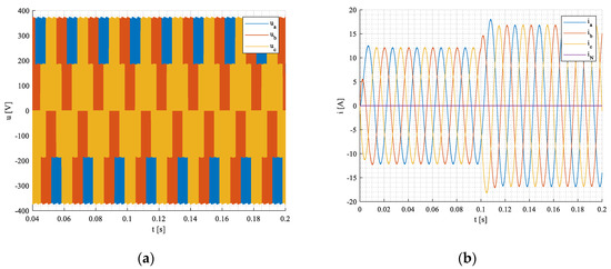
Figure 22. VSI inverter voltages (a) and currents (b) in $a,b,c$—coordinate system during the transient.

Apparent, active, blind, and distortion power components during transient states for 3-, 5-, and 2-phase systems are shown at the end of Section 3.3.

3.3.2. 5-Phase Inverter Type of VSI with Linear RL Load

Parameters for steady states at $t\in ⟨0.0;0.1⟩$ and at $t\in ⟨0.1;0.2⟩$ are given in the Table 29:

Table 29. Load parameters for steady states before and after load change.

Load	$\mathit{R} \left[\mathsf{\Omega }\right]$	$\mathit{L} \left[\mathbf{mH}\right]$	$\mathit{Z} \left[\mathsf{\Omega }\right]$	$\mathit{\tau }$$\left[\mathbf{ms}\right]$	$\mathit{\phi }$ $[°\mathbf{el}.]$	$\mathbf{c}\mathbf{o}\mathbf{s} \mathit{\phi }$$[-]$	$\mathbf{s}\mathbf{i}\mathbf{n} \mathit{\phi } [-]$
before	$18.4$	$43.93$	$23$	$2.39$	$36.76$	$0.8$	$0.6$
after	$9.2$	$43.93$	$16.59$	$4.78$	$56.33$	$0.5545$	$0.8322$

$U_{rms}=230 \mathrm{V}, f=50 \mathrm{Hz}$, 5-phase system.

Power components average values, classical calculus, assuming harmonic currents, are given in Table 30:

Table 30. Classical calculation before and after the change (at steady states).

Time	${\mathit{S}}_{1\mathit{a}\mathit{v}} \left[\mathbf{VA}\right]$	${\mathit{P}}_{1\mathit{a}\mathit{v}} \left[\mathbf{W}\right]$	${\mathit{Q}}_{1\mathit{a}\mathit{v}} \left[\mathbf{VAr}\right]$	${\mathit{D}}_{\mathit{a}\mathit{v}} [\mathbf{VAd}]$	$\mathit{P}\mathit{F} [-]$	${\mathit{A}}_1 \left[\mathbf{A}\right]$	$\mathbf{c}\mathbf{o}\mathbf{s} {\mathit{\phi }}_1 \left[\mathbf{W}\right]$
$\mathrm{t}=0.1 \mathrm{s}$	$10,141$	$8112$	$6084$	$-$	$-$	$13.30$	$0.8000$
$\mathrm{t}=0.2 \mathrm{s}$	$14,061$	$11,249$	$8436$	$-$	$-$	$18.45$	$0.5546$

$U_{1\alpha ,rms}=216 \mathrm{V}, U_{\beta 1,rms}=216 \mathrm{V},I_{1\alpha ,rms}=9.39 \mathrm{A},I_{1\beta ,rms}=9.39 \mathrm{A},I_{1\alpha ,rms}=13.02 \mathrm{A}, I_{1\beta ,rms}=13.02 \mathrm{A}$.

Simulation Results, Simulation Step 200 µs

Measurable quantities, i.e., voltages and currents in $\alpha ,\beta \left(rms\right)$, and their parameters are given in Table 31.

Table 31. Simulation results before and after the change (at steady states).

Time	${\mathit{U}}_{\mathit{\alpha },\mathit{r}\mathit{m}\mathit{s}} \left[\mathbf{V}\right]$	${\mathit{U}}_{\mathit{\beta },\mathit{r}\mathit{m}\mathit{s}} \left[\mathbf{V}\right]$	${\mathit{I}}_{\mathit{\alpha },\mathit{r}\mathit{m}\mathit{s}} \left[\mathbf{A}\right]$	${\mathit{I}}_{\mathit{\beta },\mathit{r}\mathit{m}\mathit{s}} \left[\mathbf{A}\right]$	${\mathit{A}}_1 \left[\mathbf{A}\right]$	${\mathit{\phi }}_1 \left[°\mathbf{el}.\right]$	$\mathbf{c}\mathbf{o}\mathbf{s} {\mathit{\phi }}_1 [-]$
$\mathrm{t}=0.1 \mathrm{s}$	$237.1$	$237.1$	$9.408$	$9.408$	$13.30$	$36.90$	$0.7947$
$\mathrm{t}=0.2 \mathrm{s}$	$237.1$	$237.1$	$13.05$	$13.05$	$18.45$	$56.33$	$0.5547$

For the 5-phase inverter: $U_{1,max}$(0,1) = 306.8 V, $U_{1,max}$(0,2) = 306.8 V.

Power component average values, computed in Matlab/Simulink are given in Table 32.

Table 32. Simulation results before and after the change (at steady states).

Time	${\mathit{S}}_{\mathit{a}\mathit{v}} \left[\mathbf{VA}\right]$	${\mathit{P}}_{\mathit{a}\mathit{v}} \left[\mathbf{W}\right]$	${\mathit{Q}}_{\mathit{a}\mathit{v}} \left[\mathbf{VAr}\right]$	${\mathit{D}}_{\mathit{a}\mathit{v}} [\mathbf{VAd}]$	$\mathit{P}\mathit{F} [-]$	$\mathit{T}\mathit{H}{\mathit{D}}_{\mathit{i}} [\%]$	${\mathit{P}}_{1\mathit{a}\mathit{v}} \left[\mathbf{W}\right]$	${\mathit{P}}_{0\mathit{a}\mathit{v}} \left[\mathbf{W}\right]$
$\mathrm{t}=0.1 \mathrm{s}$	$11,154.5$	$8159.6$	$6126.0$	$4507.3$	$0.7315$	$0.0$	$8106$	$0$
$\mathrm{t}=0.2 \mathrm{s}$	$15,472.0$	$7847$	$11,778.8$	$6251.2$	$0.5071$	$0.0$	$7846$	$0$

Network voltages and currents of inverter in $a,b,c,d,e$- coordinate system during transient is shown in Figure 23a,b.

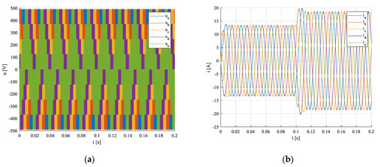
Figure 23. VSI inverter voltages (a) and currents (b) in $a,b,c,d,e$- coordinate system during the transient.

Subsequently, the voltages and currents are converted into an $\alpha , \beta$-system, and then the power components in the p-q system are calculated. Apparent, active, blind, and distortion power components during transient states for 3-, 5-, and 2-phase systems are shown in Figure 24a–d.

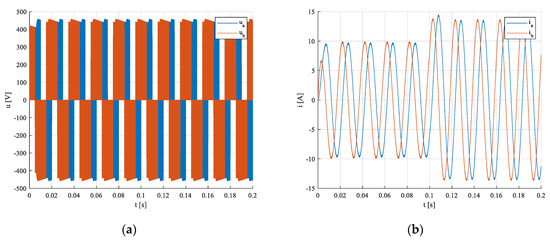
Figure 24. VSI inverter voltages (a) and currents (b) inresp. in - systems during the transient.

3.3.3. 2-Phase Inverter Type of VSI with Linear RL Load

There is a considered system having two 1- phase inverters with PWM and supplying linear RL load, as in Figure 21c.

Parameters for steady states at $t\in ⟨0.0;0.1⟩$ and at $t\in ⟨0.1;0.2⟩$ are given in the Table 33:

Table 33. Load parameters for steady states before and after load change.

Load	$\mathit{R} \left[\mathsf{\Omega }\right]$	$\mathit{L} \left[\mathbf{mH}\right]$	$\mathit{Z} \left[\mathsf{\Omega }\right]$	$\mathit{\tau }$$\left[\mathbf{ms}\right]$	$\mathit{\phi }$$[°\mathbf{el}.]$	$\mathbf{c}\mathbf{o}\mathbf{s} \mathit{\phi } [-]$	$\mathbf{s}\mathbf{i}\mathbf{n} \mathit{\phi } [-]$
before	$18.4$	$43.93$	$23$	$2.39$	$36.76$	$0.8$	$0.6$
after	$9.2$	$43.93$	$16.59$	$4.78$	$56.33$	$0.5545$	$0.8322$

U_rms = 230 V, f = 50 Hz, 2-phase system.

Power component average values, and classical calculus-assuming harmonic currents, are given in Table 34.

Table 34. Classical calculation before and after the change (at steady states).

Time	${\mathit{S}}_{1\mathit{a}\mathit{v}} \left[\mathbf{VA}\right]$	${\mathit{P}}_{1\mathit{a}\mathit{v}} \left[\mathbf{W}\right]$	${\mathit{Q}}_{1\mathit{a}\mathit{v}} \left[\mathbf{VAr}\right]$	${\mathit{D}}_{\mathit{a}\mathit{v}} [\mathbf{VAd}]$	$\mathit{P}\mathit{F} [-]$	${\mathit{A}}_1 \left[\mathbf{A}\right]$	$\mathbf{c}\mathbf{o}\mathbf{s} {\mathit{\phi }}_1 \left[\mathbf{W}\right]$
$\mathrm{t}=0.1 \mathrm{s}$	$7 597$	$6 077$	$4 558$	$-$	$-$	$18.17$	$0.8000$
$\mathrm{t}=0.2 \mathrm{s}$	$10 535$	$8 428$	$6 321$	$-$	$-$	$25.20$	$0.5546$

$U_{1\alpha ,rms}=295.6 \mathrm{V}, U_{1\beta ,rms}=295.6 \mathrm{V}, I_{1\alpha ,rms}=12.85 \mathrm{A}, I_{1\beta ,rms}=14.83 \mathrm{A}, I_{1\alpha ,rms}=17.82 \mathrm{A}, I_{1\beta ,rms}=17.82 \mathrm{A}$.

Simulation Results, Simulation Step 200 µs

Measurable quantities, i.e., voltages and currents in $\alpha ,\beta \left(rms\right)$, and their parameters are given in Table 35.

Table 35. Simulation results before and after the change (at steady states).

Time	${\mathit{U}}_{\mathit{\alpha },\mathit{r}\mathit{m}\mathit{s}} \left[\mathbf{V}\right]$	${\mathit{U}}_{\mathit{\beta },\mathit{r}\mathit{m}\mathit{s}} \left[\mathbf{V}\right]$	${\mathit{I}}_{\mathit{\alpha },\mathit{r}\mathit{m}\mathit{s}} \left[\mathbf{A}\right]$	${\mathit{I}}_{\mathit{\beta },\mathit{r}\mathit{m}\mathit{s}} \left[\mathbf{A}\right]$	${\mathit{A}}_1 \left[\mathbf{A}\right]$	${\mathit{\phi }}_1 \left[°\mathbf{el}.\right]$	$\mathbf{c}\mathbf{o}\mathbf{s} {\mathit{\phi }}_1 [-]$
$\mathrm{t}=0.1 \mathrm{s}$	$336.7$	$346.8$	$12.84$	$13.42$	$18.81$	$36.90$	$0.7947$
$\mathrm{t}=0.2 \mathrm{s}$	$337.4$	$347,3$	$17.84$	$18.63$	$26.09$	$56.33$	$0.5547$

For the 2-phase inverter: $U_{1,max}$(0,1) = 418.5 V, $U_{1,max}$(0,2) = 419.5 V.

Power component average values, computed in Matlab/Simulink are given in Table 36.

Table 36. Simulation results before and after the change (at steady states).

Time	${\mathit{S}}_{\mathit{a}\mathit{v}} \left[\mathbf{VA}\right]$	${\mathit{P}}_{\mathit{a}\mathit{v}} \left[\mathbf{W}\right]$	${\mathit{Q}}_{\mathit{a}\mathit{v}} \left[\mathbf{VAr}\right]$	${\mathit{D}}_{\mathit{a}\mathit{v}} [\mathbf{VAd}]$	$\mathit{P}\mathit{F} [-]$	$\mathit{T}\mathit{H}{\mathit{D}}_{\mathit{i}} [\%]$	${\mathit{P}}_{1\mathit{a}\mathit{v}} \left[\mathbf{W}\right]$	${\mathit{P}}_{0\mathit{a}\mathit{v}} \left[\mathbf{W}\right]$
$\mathrm{t}=0.1 \mathrm{s}$	$8975.0$	$6358.0$	$4767$	$4173$	$0.7084$	$46.5$	$6255.5$	$0$
$\mathrm{t}=0.2 \mathrm{s}$	$12,490$	$6133$	$9196$	$5816$	$0.4911$	$46.57$	$6071.6$	$0$

Network voltages and currents in $a,b$, resp. $\alpha ,\beta$- system during transient are shown in Figure 24a,b.

3.3.4. Comparison of Power Components in 2-,3- and 5-Phase Supply Systems under Inverter Supply

Apparent, active, blind, and distortion power components during transient states for 3-, 5-, and 2-phase systems are shown in Figure 25a–d.

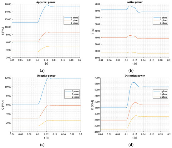
Figure 25. Apparent—(a), active—(b), blind—(c), and distortion (d) power components during transient states for 3-, 5-, and 2-phase systems under inverter-supplied linear RL load.

The simulation was performed under the same load phase parameters; therefore, the magnitudes are proportionately different.

The waveforms of apparent, active, and reactive (blind) power components during transient states for 3-, 5-, and 2-phase systems look similar to those under harmonic supply (Figure 11a–d). However, the distortion component of power is different substantively and features nearly 42% of total power. Therefore, the supply voltages of the inverters were adapted to be the total apparent power the same as under harmonic supply (approx. 16 kVA/5-phase system, Figure 25a vs. Figure 11a). The reason was an easier comparison between inverter- and harmonic supply. During the transient state, the distortion component is characterized by a typical overshoot, Figure 25d. Note to create the 2-phase inverter network. Two single full-bridge inverters were used. Distortion components of all connections are rather high due to the impulse character of the voltages produced by VSI inverters. Therefore, the power factors are also rather poor.

The reference currents $i_{\alpha ref}\left(k\right)$ and $i_{\beta ref}\left(k\right)$ for compensating by power active filter (PAF compensator) are calculated using Equation (27a,b). Before this, they should be back-transformed into $a, b, c$-phase system.

3.4. Mode #4 Non-Harmonic Supply and Nonlinear Load

3.4.1. Symmetrical Network, Non-Symmetric Load

The load asymmetry has been provided by step change of the resistor $R_a=18.4 \mathsf{\Omega }$ to 9.2 Ω in phase a at the time of 0.1 s (after settling).

Parameters for steady states at $t\in ⟨0.0;0.1⟩$ and at $t\in ⟨0.1;0.2⟩$ are given in the Table 37:

Table 37. Load parameters for steady states before and after load change.

Load	${\mathit{R}}_{\mathit{a}}$ $\left[\mathsf{\Omega }\right]$	$\mathit{L} \left[\mathbf{mH}\right]$	$\mathit{Z} \left[\mathsf{\Omega }\right]$	${\mathit{\tau }}_{\mathit{a}}$$\left[\mathbf{ms}\right]$	${\mathit{\phi }}_{\mathit{a}}$$[°\mathbf{el}.]$	$\mathbf{c}\mathbf{o}\mathbf{s} {\mathit{\phi }}_{\mathit{a}}$$[-]$	$\mathbf{s}\mathbf{i}\mathbf{n} {\mathit{\phi }}_{\mathit{a}} [-]$
before	$18.4$	$43.93$	$23$	$2.39$	$36.76$	$0.8$	$0.6$
after	$9.2$	$43.93$	$16.59$	$4.78$	$56.33$	$0.5545$	$0.8322$

$U_{rms}=230 \mathrm{V}, f=50 \mathrm{Hz}$, 3-phase system.

Simulation Results Using Matlab/Simulink, Simulation Step 200 µs

Measurable quantities, i.e., voltages and currents in $\alpha ,\beta \left(rms\right)$, and their parameters are given in Table 38.

Table 38. Simulation results before and after the change (at steady states).

Time	${\mathit{U}}_{\mathit{\alpha },\mathit{r}\mathit{m}\mathit{s}}\left[\mathbf{V}\right]$	${\mathit{U}}_{\mathit{\beta },\mathit{r}\mathit{m}\mathit{s}}\left[\mathbf{V}\right]$	${\mathit{U}}_{0,\mathit{r}\mathit{m}\mathit{s}}\left[\mathbf{V}\right]$	${\mathit{I}}_{\mathit{\alpha },\mathit{r}\mathit{m}\mathit{s}}\left[\mathbf{A}\right]$	${\mathit{I}}_{\mathit{\beta },\mathit{r}\mathit{m}\mathit{s}}\left[\mathbf{A}\right]$	${\mathit{I}}_{0,\mathit{r}\mathit{m}\mathit{s}}\left[\mathbf{A}\right]$
$\mathrm{t}=0.1 \mathrm{s}$	$229.7$	$229.8$	$0$	$9.971$	$9.998$	$0$
$\mathrm{t}=0.2 \mathrm{s}$	$229.7$	$229.7$	$0$	$12.42$	$9.991$	$1.846$

$R_a$ changed from $18.4 \mathsf{\Omega }$ to $9.2 \mathsf{\Omega }$ at 0.2 s.

Power component average values, computed in Matlab/Simulink are given in Table 39.

Table 39. Simulation results before and after the change (at steady states).

Time	${\mathit{S}}_{\mathit{a}\mathit{v}} \left[\mathbf{VA}\right]$	${\mathit{P}}_{\mathit{a}\mathit{v}} \left[\mathbf{W}\right]$	${\mathit{Q}}_{\mathit{a}\mathit{v}} \left[\mathbf{VAr}\right]$	${\mathit{D}}_{\mathit{a}\mathit{v}} [\mathbf{VAd}]$	$\mathit{P}\mathit{F} [-]$	${\mathit{P}}_{0\mathit{a}\mathit{v}} \left[\mathbf{W}\right]$	$\mathit{T}\mathit{H}{\mathit{D}}_{\mathit{i}} [\%]$
$\mathrm{t}=0.1 \mathrm{s}$	$6888$	$5510$	$4134$	$0$	$0.8$	$0$	$0.0$
$\mathrm{t}=0.2 \mathrm{s}$	$7727$	$5442$	$5404$	$957$	$0.7039$	$0$	$12.39$

Network voltages and currents in $a,b,c,N$-coordinate system at steady-states are shown in Figure 26a,b.

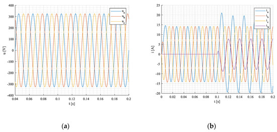
Figure 26. Network voltages (a), load, and neutral currents (b).

Apparent, active, blind, and distortion power components during transient states for a 3 –phase system are shown in Figure 27a–d.

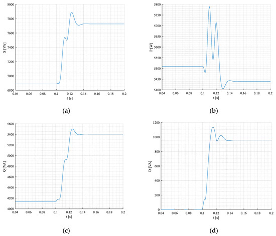
Figure 27. Apparent-(a), active-(b), blind-(c), and distortion (d) power components during transient states for 3-phase system under a symmetrical network supplying non-symmetrical linear RL load.

In this case, the network neutral is connected to the load neutral. Therefore, current I_N flows through the neutral wire despite the voltage zero-sequence being zero. It is interesting that active power in steady state after the transient is a little bit smaller than before, Figure 27b, although load resistance in phase “a” was changed to one-half. However, the phase current i_a and current of neutral I_N are in antiphase (shifted by 180° el.), Figure 27b. So, the power loss (Joule loss) in neutral wire acts negatively on the load active power. During the transient state, waveforms feature oscillating characters, and power component $Po$ is zero due to zero-sequence component $Uo$ equal to zero.

3.4.2. Non-Symmetric Network, Symmetrical Load

The network asymmetry has been provided by a step change of voltage in phase a from 325 V by 33% at the time 0.1 sec (after settling).

Parameters for steady states at $t\in ⟨0.0;0.1⟩$ and at $t\in ⟨0.1;0.2⟩$ are given in the Table 40:

Table 40. Load parameters for steady states before and after load change.

Load	${\mathit{R}}_{\mathit{a}}$ $\left[\mathsf{\Omega }\right]$	$\mathit{L} \left[\mathbf{mH}\right]$	$\mathit{Z} \left[\mathsf{\Omega }\right]$	${\mathit{\tau }}_{\mathit{a}}$$\left[\mathbf{ms}\right]$	${\mathit{\phi }}_{\mathit{a}}$$[°\mathbf{el}.]$	$\mathbf{c}\mathbf{o}\mathbf{s} {\mathit{\phi }}_{\mathit{a}}$$[-]$	$\mathbf{s}\mathbf{i}\mathbf{n} {\mathit{\phi }}_{\mathit{a}} [-]$
before	$18.4$	$43.93$	$23$	$2.39$	$36.76$	$0.8$	$0.6$
after	$9.2$	$43.93$	$16.59$	$4.78$	$56.33$	$0.5545$	$0.8322$

$U_{rms}=230 \mathrm{V}, f=50 \mathrm{Hz}$, 3-phase system.

Simulation Results Using Matlab/Simulink, Simulation Step 200 µs

Measurable quantities, i.e., voltages and currents in $\alpha ,\beta \left(rms\right)$, and their parameters are given in Table 41.

Table 41. Simulation results before and after the change (at steady states).

Time	${\mathit{U}}_{\mathit{\alpha },\mathit{r}\mathit{m}\mathit{s}} \left[\mathbf{V}\right]$	${\mathit{U}}_{\mathit{\beta },\mathit{r}\mathit{m}\mathit{s}} \left[\mathbf{V}\right]$	${\mathit{U}}_{0,\mathit{r}\mathit{m}\mathit{s}} \left[\mathbf{V}\right]$	${\mathit{I}}_{\mathit{\alpha },\mathit{r}\mathit{m}\mathit{s}} \left[\mathbf{A}\right]$	${\mathit{I}}_{\mathit{\beta },\mathit{r}\mathit{m}\mathit{s}} \left[\mathbf{A}\right]$	${\mathit{I}}_{0,\mathit{r}\mathit{m}\mathit{s}} \left[\mathbf{A}\right]$
$\mathrm{t}=0.1 \mathrm{s}$	$229.5$	$230.1$	$0$	$10.01$	$9.969$	$0$
$\mathrm{t}=0.2 \mathrm{s}$	$306.1$	$230.1$	$38.26$	$13.33$	$9.986$	$1.666$

$U_{a,max}$ changed from 325 V to 432 V (by 33%).

Power component average values, computed in Matlab/Simulink are given in Table 42.

Table 42. Simulation results before and after the change (at steady states).

Time	${\mathit{S}}_{\mathit{a}\mathit{v}} \left[\mathbf{VA}\right]$	${\mathit{P}}_{\mathit{a}\mathit{v}} \left[\mathbf{W}\right]$	${\mathit{Q}}_{\mathit{a}\mathit{v}} \left[\mathbf{VAr}\right]$	${\mathit{D}}_{\mathit{a}\mathit{v}} [\mathbf{VAd}]$	$\mathit{P}\mathit{F} [-]$	${\mathit{P}}_{0\mathit{a}\mathit{v}} \left[\mathbf{W}\right]$	$\mathit{T}\mathit{H}{\mathit{D}}_{\mathit{i}} [\%]$
$\mathrm{t}=0.1 \mathrm{s}$	$6888$	$5510$	$4134$	$0$	$0.8$	$0$	$0.0$
$\mathrm{t}=0.2 \mathrm{s}$	$9567$	$7729$	$5511$	$1186$	$0.8079$	$51.02$	$12.4$

Network voltages and currents in $a,b,c$- coordinate system at steady states are shown in Figure 28a,b.

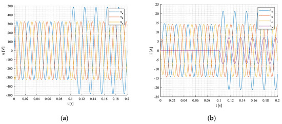
Figure 28. Network voltages (a), load, and neutral currents (b).

Apparent-, active-, blind-, and distortion power components during transient states for a 3-phase system are shown in Figure 29a–d.

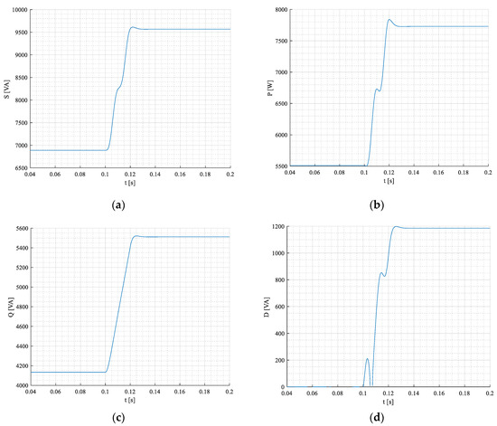
Figure 29. Apparent- (a), active-(b), blind-(c), and distortion (d)power components during transient states for the 3-phase system under inverter-supplied non-symmetrical linear RL load.

Zero power component $Po$ is not equal to zero, and it is shown in Figure 30.

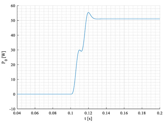
Figure 30. The waveform of zero power component Po.

Unlikely previous cases, the network voltages feature zero-sequence since $u_a$ is 33% higher, Figure 28a. Thus, the active power of the load is proportionally higher, Figure 28b, despite the phase current i_a and current of neutral I_N being in antiphase as in a non-symmetrical load case. So, this time the zero-sequence component Po is not zero, and it shows a little bit more than 50 W, Figure 30.

Compensation of reactive and distortion power in the case of non-symmetry systems needs 4-leg PAF instead of three. Calculation of reference currents for such a PAF configuration is similar to Equation (27a,b) but needs to consider zero-sequence components Equation (22), and it is done, e.g., [8,9,27].

4. Discussion

Among the most interesting worked-out result belongs to the generated distortion component during the transient of the harmonic supply linear load (mode M1a Figure 11d), while at steady state, it is zero. In the case of long system time constants (lightly loaded large motors, induction furnaces) and the need for precise compensation, it is, therefore, necessary to compensate for deformation power, although we consider a balanced network and linear RL load. Under rectifier supply system Mode #2, in the case of the apparent power component (Figure 20a), nearly the same apparent powers of 3- and 5- phase systems are generated at steady-state $t\in ⟨0.0;0.1⟩$ despite DC powers being different. Distortion components of all connections are rather high due to impulse current taken from the network. Therefore, the power factors are rather poor. In Mode #3, under non-harmonic inverter supply, distortion components of all connections are rather high due to the impulse character of the voltages produced by VSI inverters. Therefore, the power factors are also rather poor. In the case of the Mode #4 version ‚a‘, the harmonic network supplies an unbalanced load. The current I_N flows through the neutral wire despite the voltage zero-sequence being zero. It flows from an unbalanced load to a symmetrical network. Mode #4 version, b‘, the unbalanced harmonic network supplies the symmetrical linear load. The active power of the load is proportionally higher, Figure 29b, and the zero-sequence component $Po$ is added to the phase active power.

If compensating reactive blind power under linear RL load using static compensator SC (Figure 31a), the distortion power component has still remained during transient, Figure 31b,c. SC compensator comprises capacitors switched on by antiparallel thyristors at zero voltage crossing.

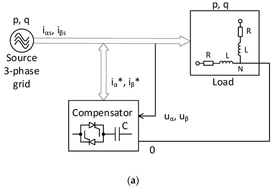
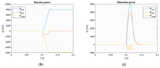
Figure 31. Using switched capacitors (a) for compensating reactive blind power (b) under linear RL load and distortion power (c).

If compensating reactive power (blind and distortion) under linear RL load using an active PAF compensator (Figure 32a), the distortion power component is compensated already during transient, Figure 32b,c. The PAF compensator comprises 3-, 5-, and 2-phase voltage inverters and DC link capacitor C.

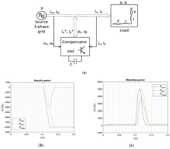
Figure 32. Using PAF active filter (a) for compensating reactive blind power (b) under linear RL load and distortion power (c).

In this case of using an active PAF compensator, if the transient was significantly longer than the time period (e.g., ten times), the deformation power would be fully compensated already during the transient state.

5. Conclusions

The paper shows the behavior of power electronic systems as well as power systems under transient states presented by step change of the load or another quantity, using the instantaneous reactive power p-q method. The simulation was performed under different types of loads and supply voltages (linear and non-linear load, sinusoidal and non-sinusoidal voltage). There are shown the simulation results with the quasi-instantaneous determination of power components’ mean values, including phase shift of fundamentals ${\phi }_1$(resp. cos ${\phi }_1)$ and total power factor $PF$. The waveform of apparent, active, blind, and distorted power components are displayed in the timeline. As has been shown, the distortion power components are generated during transient also under harmonic supply conditions and linear load.

The moving average- and moving rms methods have been used for determining a power component’s mean values in the next calculation step directly from measurable phase current and voltage quantities. Thus, using those methods and the direct measurement of a voltage and current in $\alpha ,\beta$ orthogonal system, we can calculate acting variable quantity for compensating or filtering any undesirable power components such as blind-, distortion, or total reactive power. This is important for active power filters mainly for their dynamics. Of course, all simulated power component waveforms will be then quite different from those displayed in the paper without compensation.

References

- Dugan, R.C.; McGranaghan, M.F.; Santoso, S.; Beaty, H.W. Electrical Power Systems Quality, 2nd ed.; McGrow-Hill Copyrighted Material: McGraw Hill, UK, 2004. [Google Scholar]
- Halpin, S.M.; Card, A. Power Quality. In Power Electronics Handbook, 1st ed.; Rashid, M.H., Ed.; Academic Press: San Diego, CA, USA, 2001; pp. 817–828. [Google Scholar]
- Kryltcov, S.; Makhovikov, A.; Korobitcyna, M. Novel Approach to Collect and Process Power Quality Data in Medium-Voltage Distribution Grids. Symmetry 2021, 13, 460. [Google Scholar] [CrossRef]
- León-Martínez, V.; Montañana-Romeu, J.; Peñalvo-López, E.; Valencia-Salazar, I. Relationship between Buchholz’s Apparent Power and Instantaneous Power in Three-Phase Systems. Appl. Sci. 2020, 10, 1798. [Google Scholar] [CrossRef]
- Fetea, R.; Petroianu, A. Reactive power: A Strange Concept? In Proceeding of the Second European Conference on Physics Teaching in Engineering Education, PTEE2000, Budapest, Hungary, 14–17 June 2000.
- Czarnecki, L.S. What is Wrong with the Conservative Power Theory (CPT). In Proceedings of the ICATE International Conference on Applied and Theoretical Electricity, Craiova, Romania, 6–8 October 2016. [Google Scholar] [CrossRef]
- Akagi, H.; Kanazawa, Y.; Nabae, A. Generalized Theory of the Instantaneous Reactive Power in Three-Phase Circuits. In Proceedings of the IPEC Conference, Tokyo, Japan, 27–31 March 1983; pp. 1375–1386. [Google Scholar]
- Akagi, H.; Watanabe, E.H.; Aredes, M. Instantaneous Power Theory and Applications to Power Conditioning; John Wiley & Sons-IEEE Press: New Jersey, NJ, USA, 2017; ISBN 9781119307204. [Google Scholar]
- Herrera, R.S.; Salmeron, P. Instantaneous reactive power theory: A reference in the nonlinear loads compensation. IEEE Trans. Ind. Electron. 2009, 56, 2015–2022. [Google Scholar] [CrossRef]
- Green, T.C.; Marks, J.H. Control techniques for active power filters. IEE Proc. —Electr. Power Appl. 2005, 152, 369–381. [Google Scholar] [CrossRef]
- Soares, V.; Verdelho, P.; Marques, G.D. An instantaneous active and reactive current component method for active filters. IEEE IEEE Trans. Power Electron 2000, 15, 660–669. [Google Scholar] [CrossRef]
- Dobrucky, B.; Kascak, S.; Frivaldsky, M.; Prazenica, M. Determination and compensation of non-active torques for parallel HEV using PMSM/IM motor(s). Energy 2021, 14, 2781. [Google Scholar] [CrossRef]
- Komatsu, Y. Application of the extension p-q theory to a mains-coupled photovoltaic system. In Proceedings of the Power Conversion Conference (PCC), Osaka, Japan, 2–5 April 2002; pp. 816–821. [Google Scholar] [CrossRef]
- Pipiska, M. Research of Circuitry Topologies for 3-Phase PFCs. Ph.D. Thesis, University of Žilina, Žilina, Slovak Republic, 2020. (In Slovak). [Google Scholar]
- Davidek, V.; Leipert, M.; Vlcek, M. Analogue and Digital Filters; CVUT Publisher: Czech, Prague, 2006; ISBN 80-01-03026-1. (In Czech) [Google Scholar]
- Moudgalya, K.M. Digital Control; J. Wiley & Sons: Hoboken, NJ, USA, 2007; ISBN 978-0-470-03143-8. [Google Scholar]
- Dobrucky, B.; Pokorny, M. Highest Dynamics and Ultra Fast Start-Up of Single-Phase PAF Using Virtual Approach. In IREE—International Review of Electrical Engineering; Praise Worthy Prize Publisher (IT): Naples, Campania, Italy, 2006; Volume 1, pp. 391–399. ISSN 1827-6660. [Google Scholar]
- Imam, A.A.; Kumar, R.S.; Al-Turki, Y.A. Modeling and Simulation of a PI Controlled Shunt Active Power Filter for Power Quality Enhancement Based on P-Q Theory. Electron. 2020, 9, 637. [Google Scholar] [CrossRef]
- Sozaňski, K.P. Sliding DFT Control Algorithm for Three-Phase Active Power Filter. In Proceedings of the 21st Annual IEEE Applied Power Electronics Conference and Exposition APEC ’06, Dallas, TX, USA, 19–23 March 2006. [Google Scholar] [CrossRef]
- Osowski, S. Neural network for estimation of harmonic components in a power system. IEE Proc. GTD 1992, 139, 129–135. [Google Scholar] [CrossRef]
- IEC Standard 61000-2-2; Electromagnetic Compatibility (EMC)-Part 2-2: Environment-Compatibility Levels for Low-Frequency Conducted Disturbances and Signalling in Public Low-Voltage Power Supply Systems. IEC: Geneva, Switzerland, 2002.
- Blagouchine, I.V.; Moreau, E. Analytic method for the computation of the total harmonic distortion by the Cauchy method of residues. IEEE Trans. Commun. 2011, 59, 2478–2491. [Google Scholar] [CrossRef]
- Dobrucký, B.; Chernoyarov, O.V.; Marcokova, M. Computation of the total harmonic distortion of impulse system quantities using infinite series. In Proceedings of the 14th Conference on Applied Mathematics, Bratislava, Slovakia, 3–5 February 2015; pp. 213–220. [Google Scholar]
- IEEE Standard STD 519-2014; IEEE Recommended Practice and Requirements for Harmonic Control in Electric Power Systems, IEEE Power and Energy Society, 27 March 2014. IEEE: Piscataway, NJ, USA, 2014.
- Czarnecki, L.S. Effect of supply voltage asymmetry on IRP p-q based switching compensator control. IET Power Electron. 2010, 3, 11–17. [Google Scholar] [CrossRef]
- Pavlanin, R.; Dobrucky, B.; Spanik, P. Investigation of Compensation Effect of Shunt Active Power Filter Working under the Non-Sinusoidal Voltage Conditions. In IREE—International Review of Electrical Engineering; Praise Worthy Prize Publisher (IT): Naples, Campania, Italy, 2009; Volume 4, ISSN 1827-6660. [Google Scholar]
- Acha, E.; Agelidis, V.G.; Anaya, O.; Miller, T.J.E. Power Electronic Control in Electrical Systems. In Newnes Power Engineering Series; Newnes Publisher: Oxford, UK, 2002. [Google Scholar] [CrossRef]
Publisher’s Note: MDPI stays neutral with regard to jurisdictional claims in published maps and institutional affiliations. |
© 2022 by the authors. Licensee MDPI, Basel, Switzerland. This article is an open access article distributed under the terms and conditions of the Creative Commons Attribution (CC BY) license (https://creativecommons.org/licenses/by/4.0/).