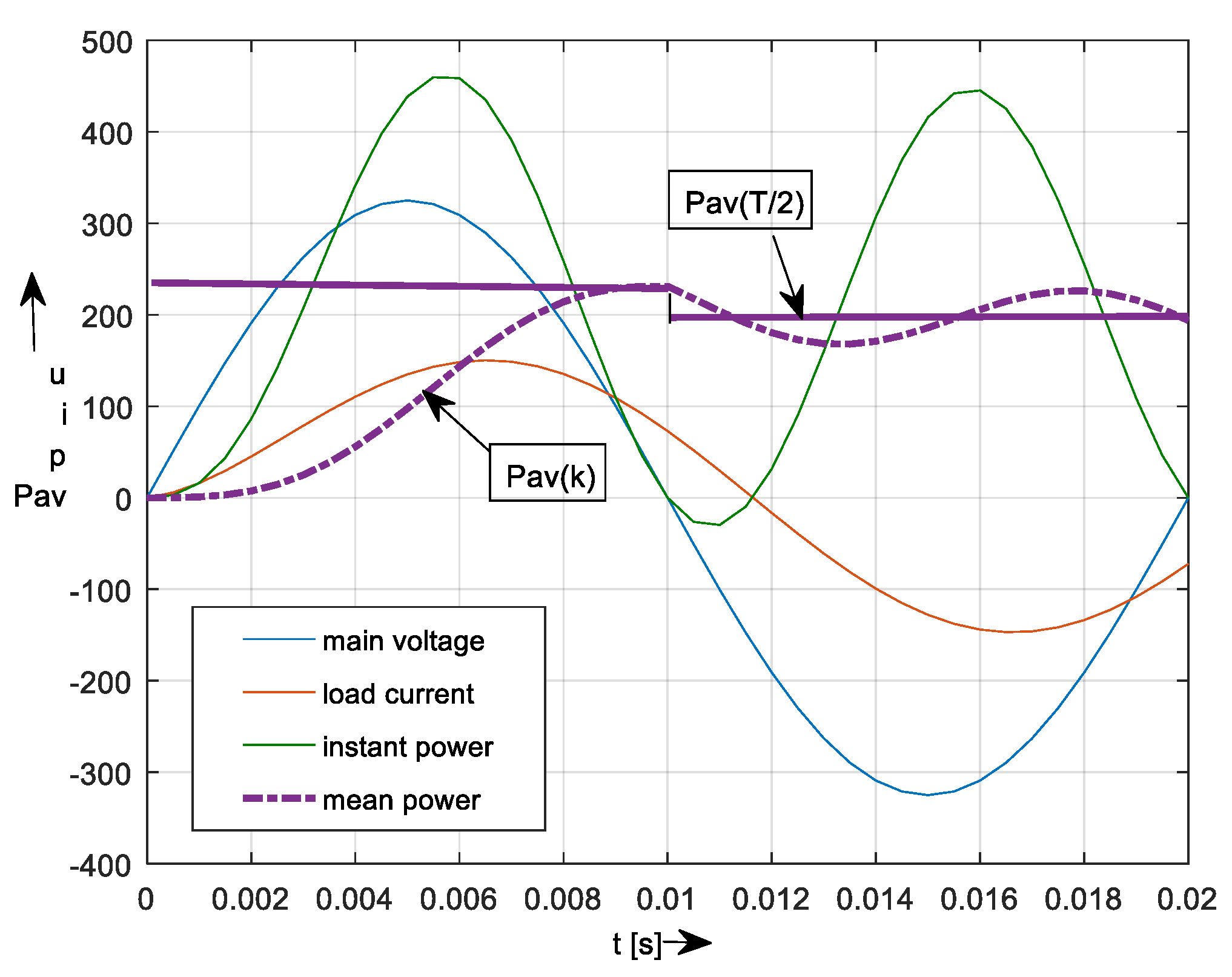
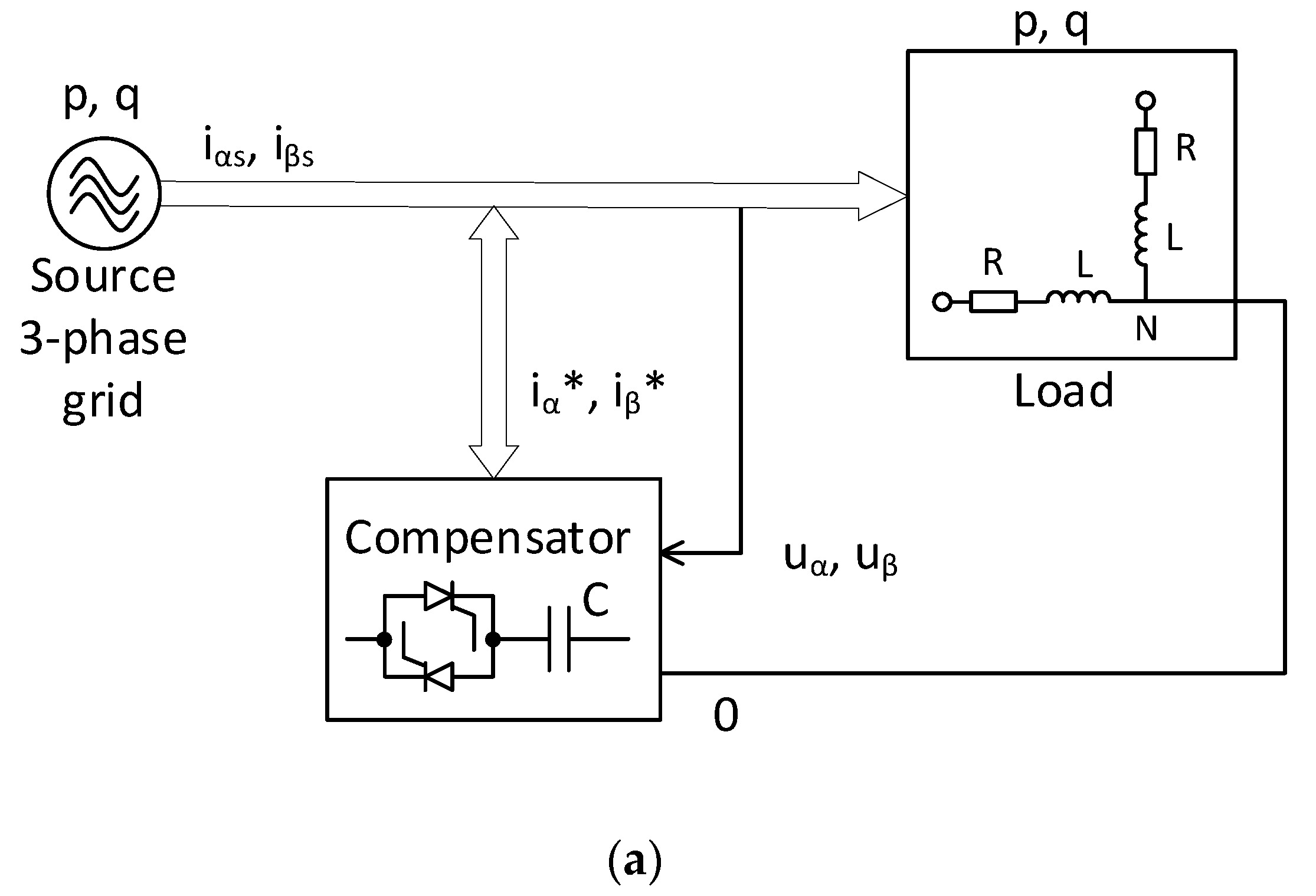
Figure 1.
Principal time-waveform of by using of MAF method: step ms, length of sliding window s.
Figure 1.
Principal time-waveform of by using of MAF method: step ms, length of sliding window s.
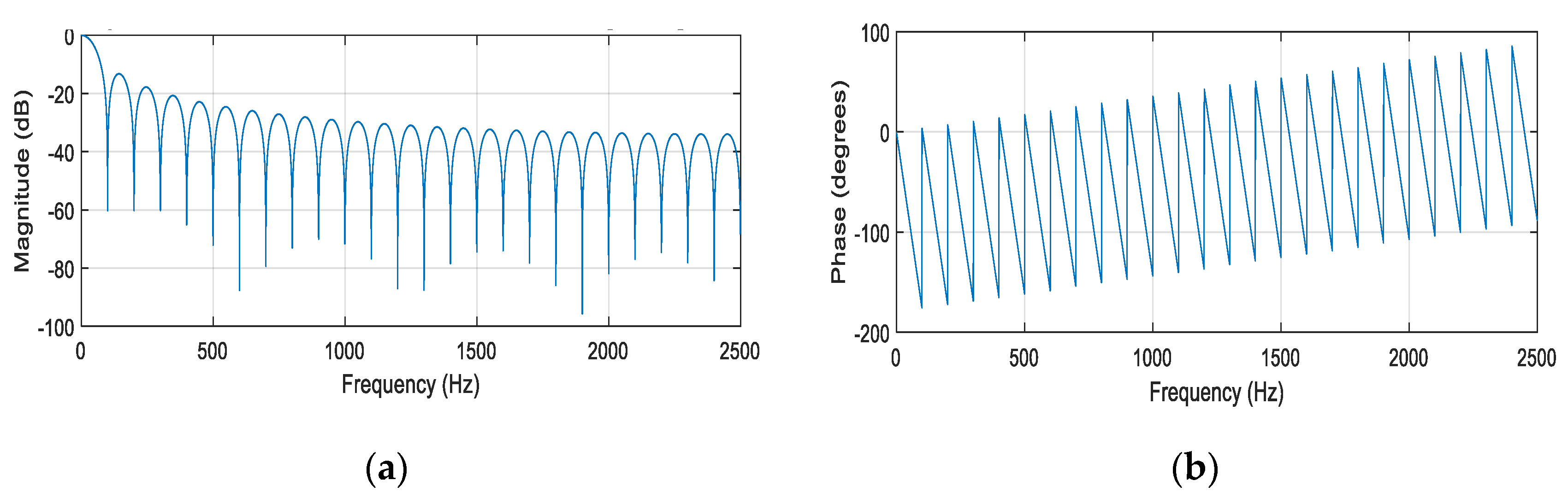
Figure 2.
Amplitude—(a) and phase—(b) frequency characteristics of DFIR filter.
Figure 2.
Amplitude—(a) and phase—(b) frequency characteristics of DFIR filter.
Figure 3.
Amplitude—(a) and phase—(b) frequency characteristics of MAF filter.
Figure 3.
Amplitude—(a) and phase—(b) frequency characteristics of MAF filter.
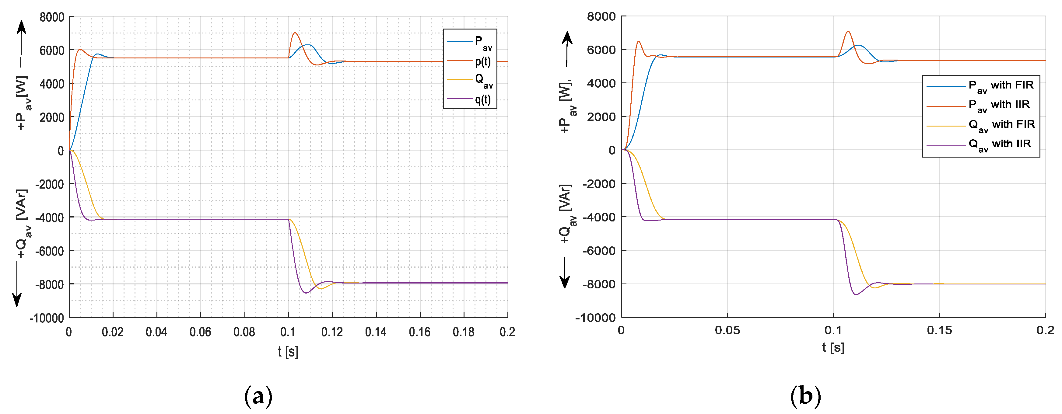
Figure 4.
Comparison of power waveforms calculated by different methods MAF and direct function in the time domain and —(a), DFIR and DIIR filters for and —(b).
Figure 4.
Comparison of power waveforms calculated by different methods MAF and direct function in the time domain and —(a), DFIR and DIIR filters for and —(b).
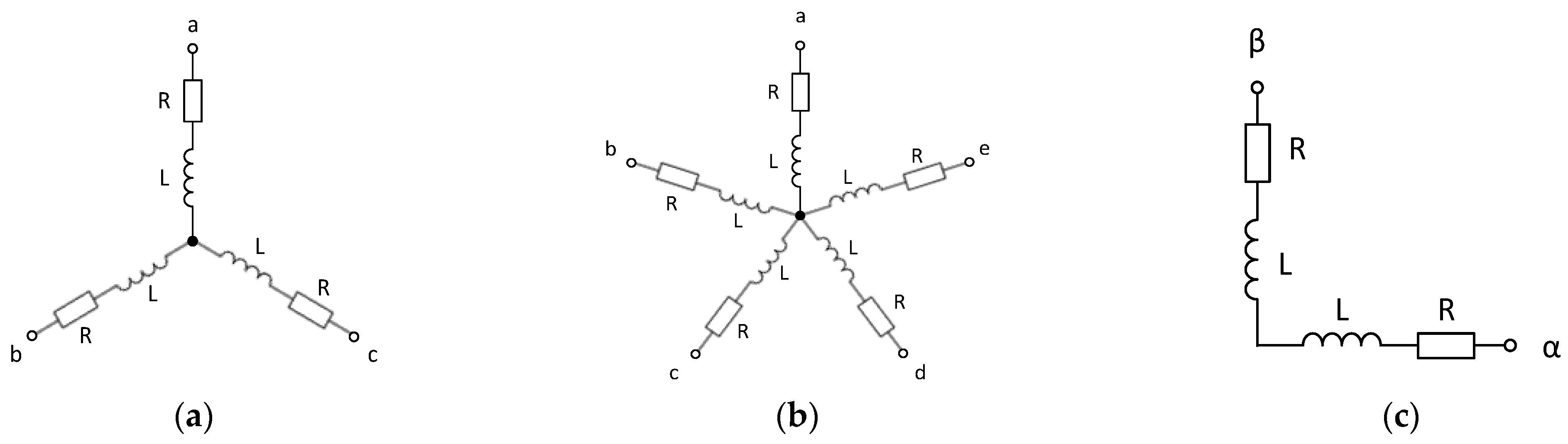
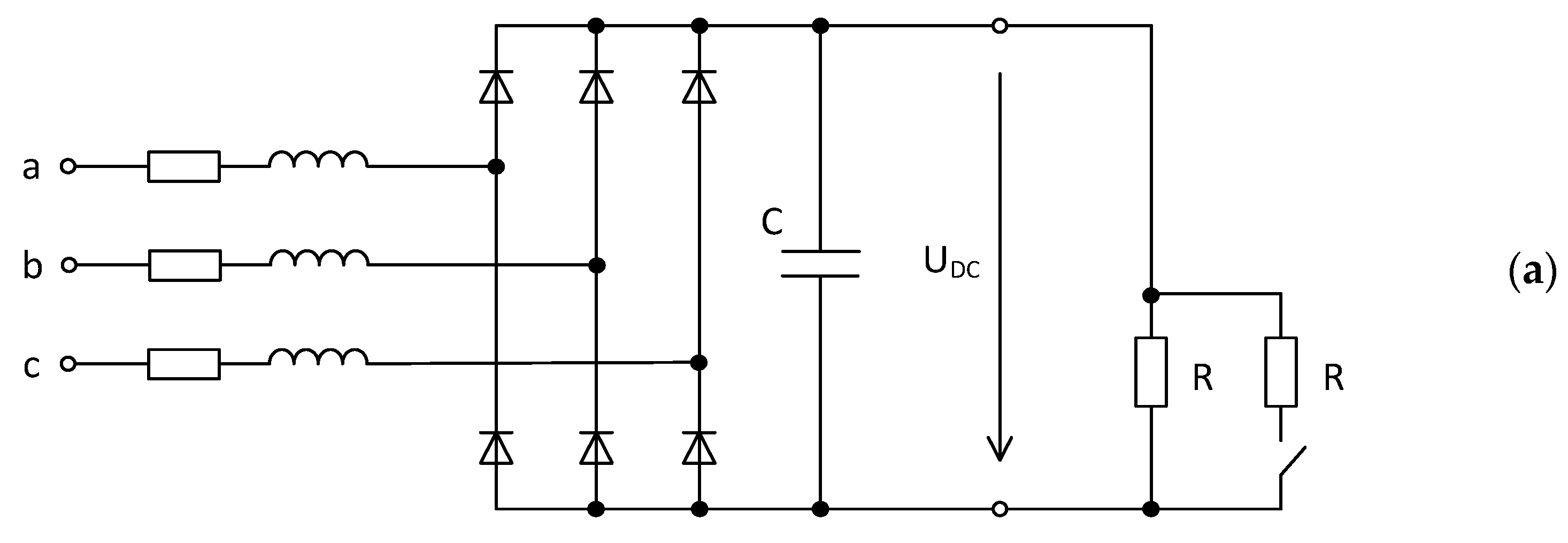
Figure 5.
The basic scheme of the considered linear RL load for 3- (a), 5- (b), and 2- (c) phase systems.
Figure 5.
The basic scheme of the considered linear RL load for 3- (a), 5- (b), and 2- (c) phase systems.
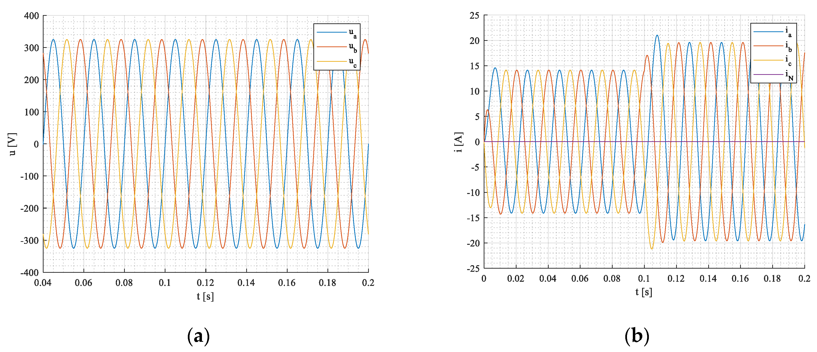
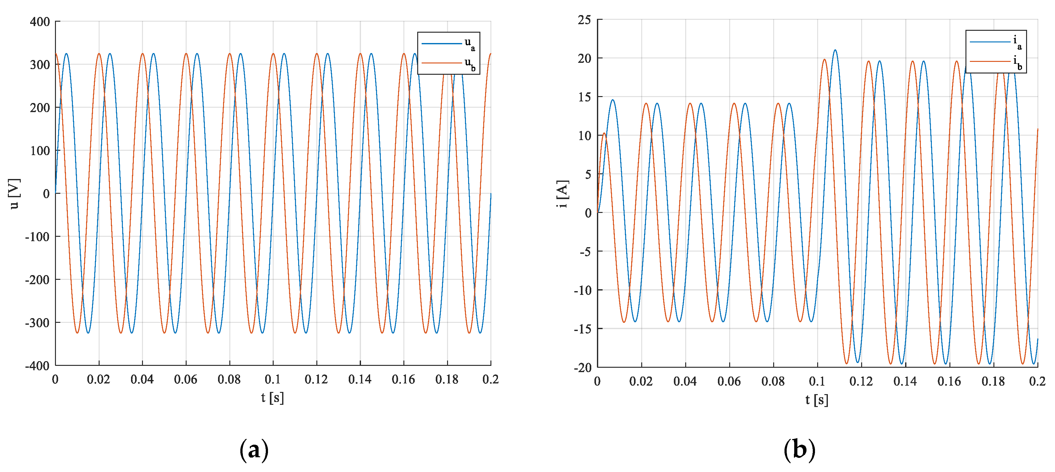
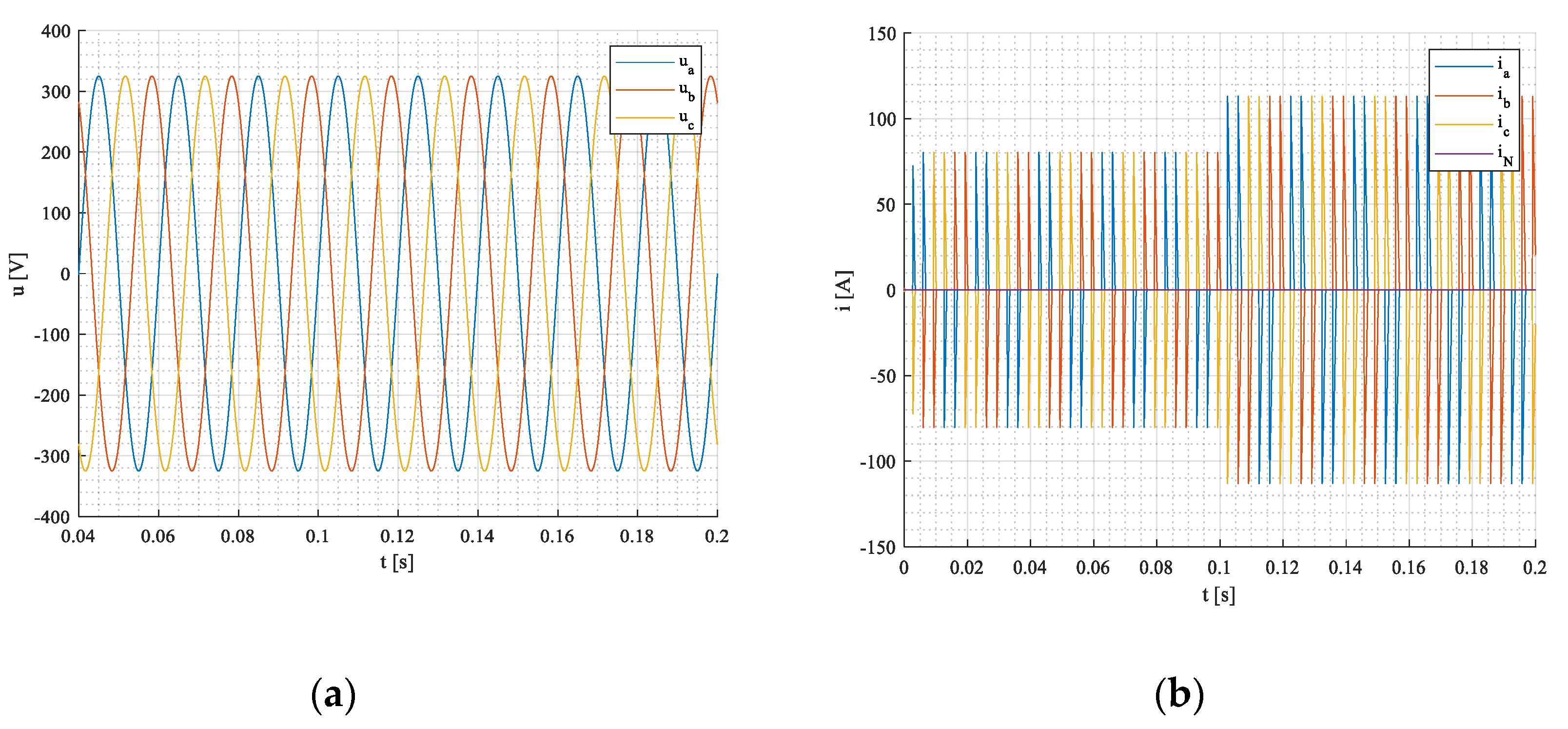
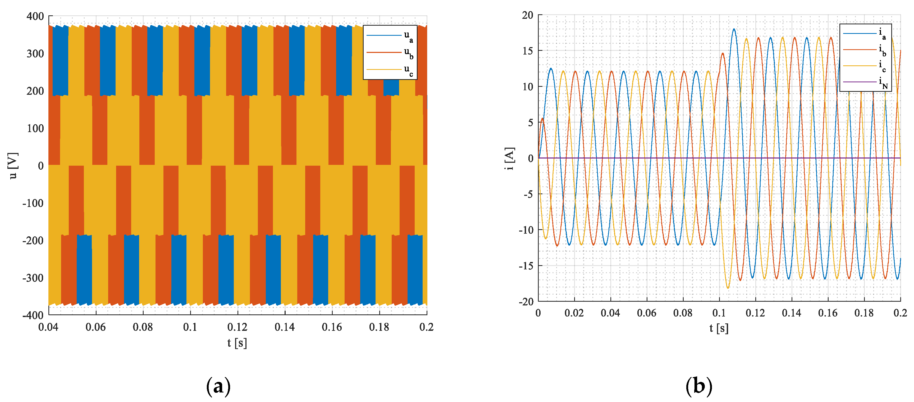
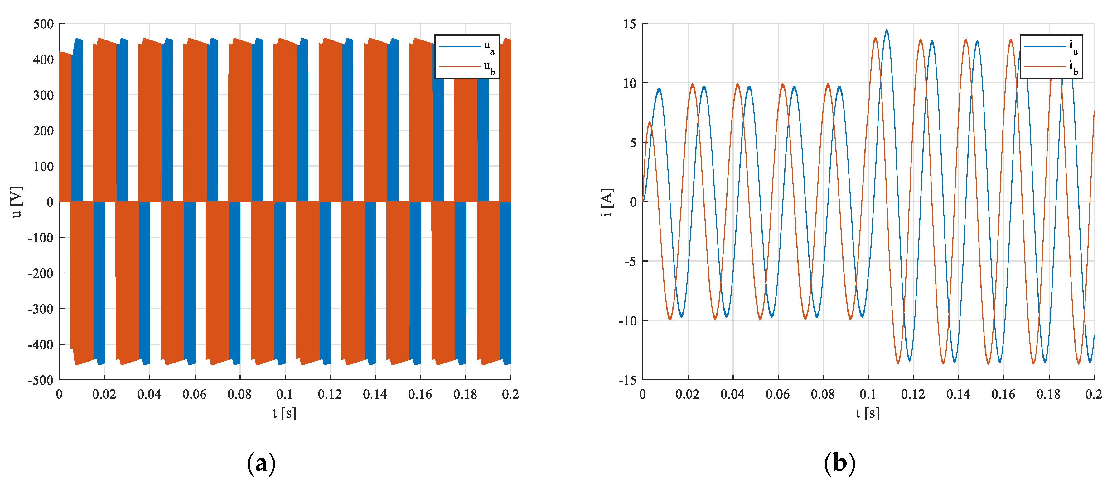
Figure 6.
Phase voltages (a), currents (b) in a,b,c—coordinates.
Figure 6.
Phase voltages (a), currents (b) in a,b,c—coordinates.
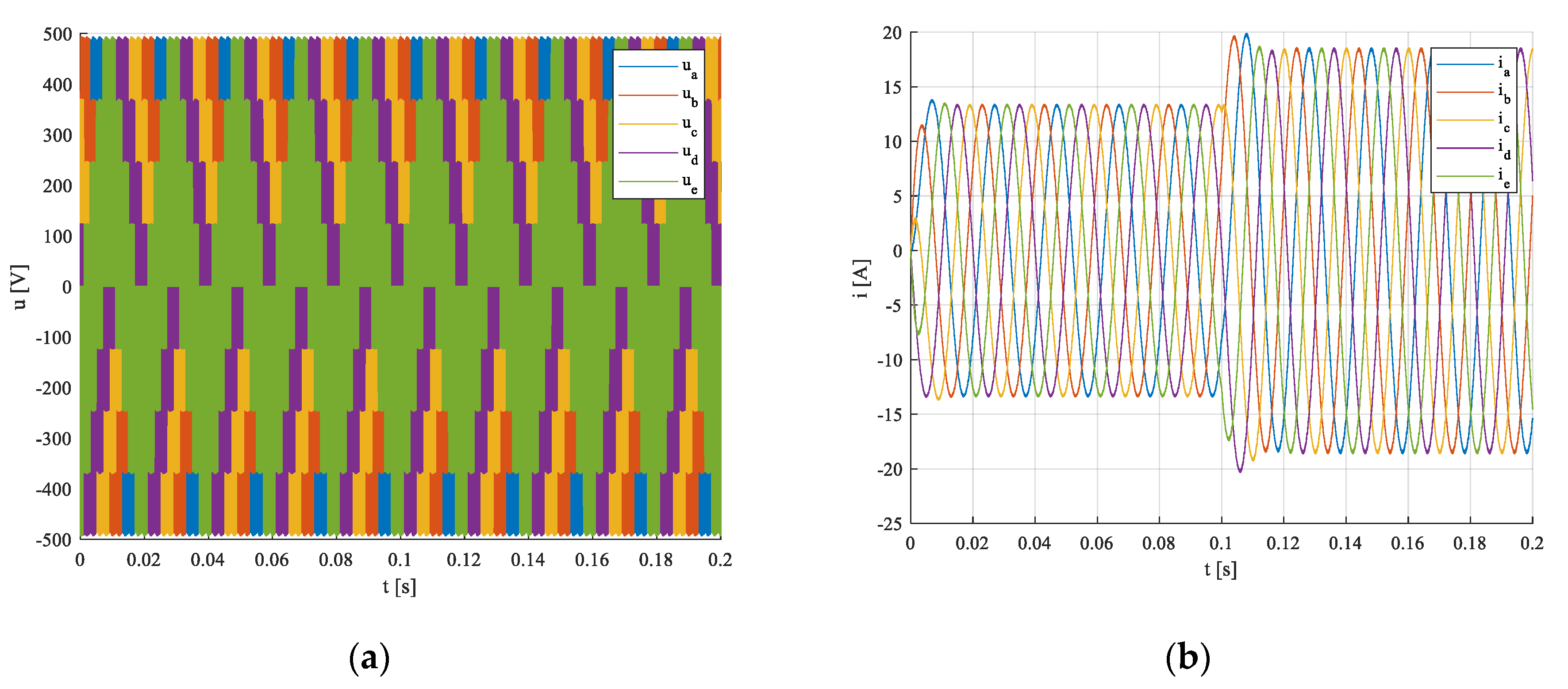
Figure 7.
Phase voltages (a), currents (b) in a,b,c—coordinates.
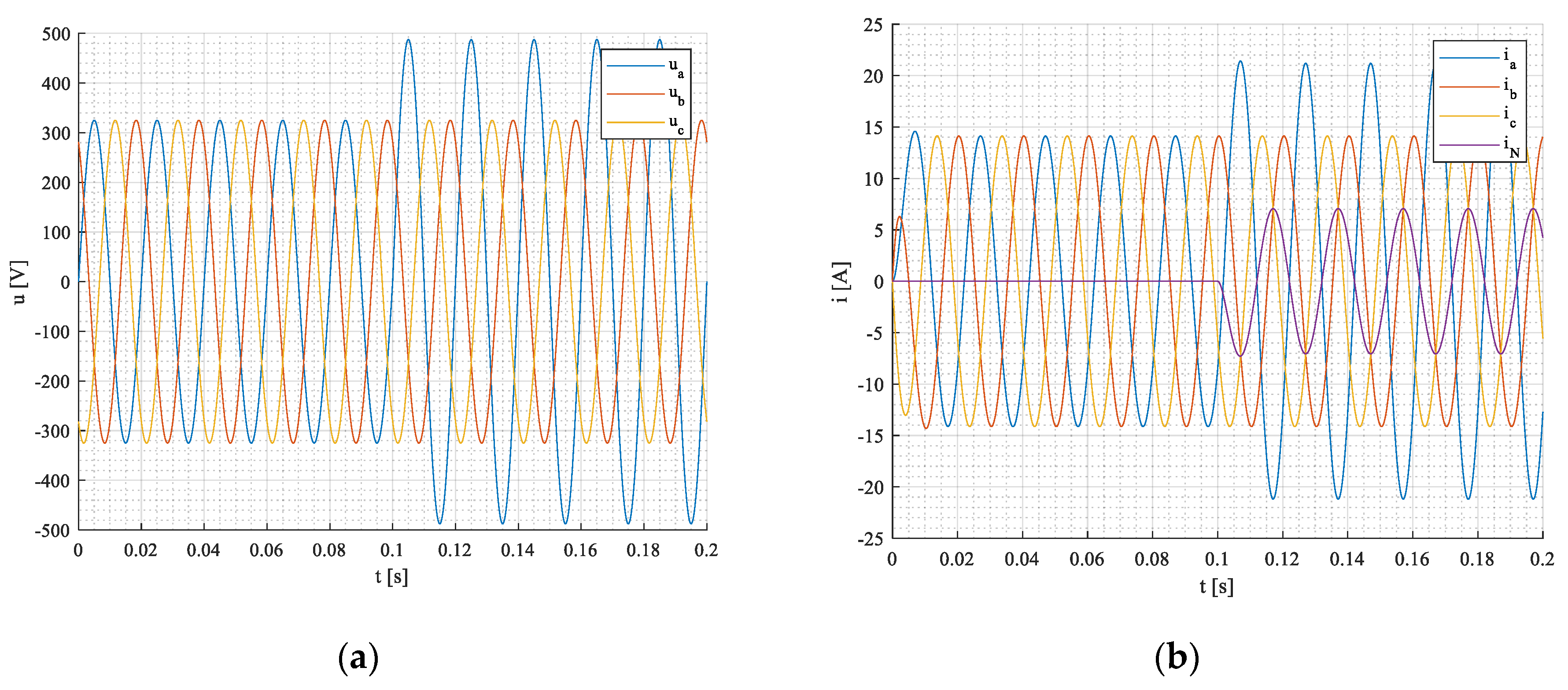
Figure 7.
Phase voltages (a), currents (b) in a,b,c—coordinates.
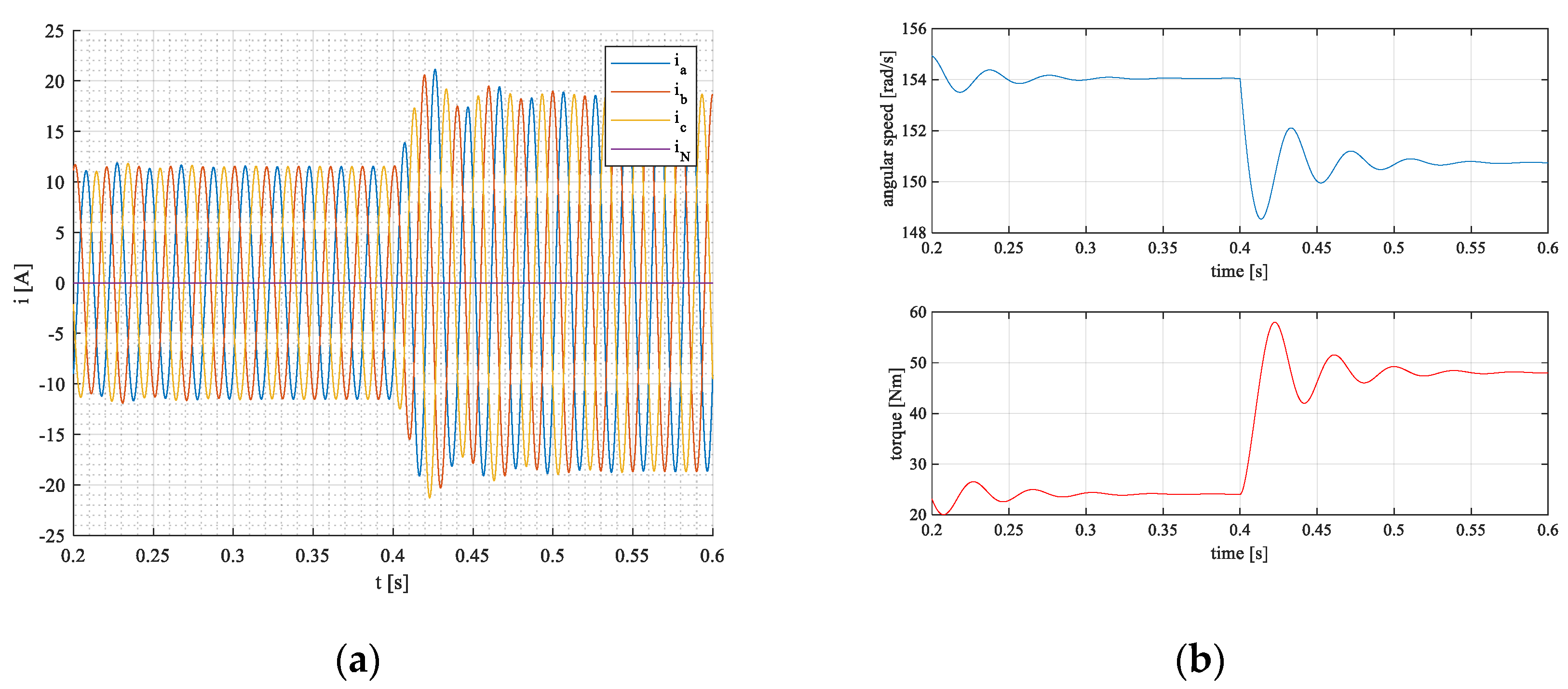
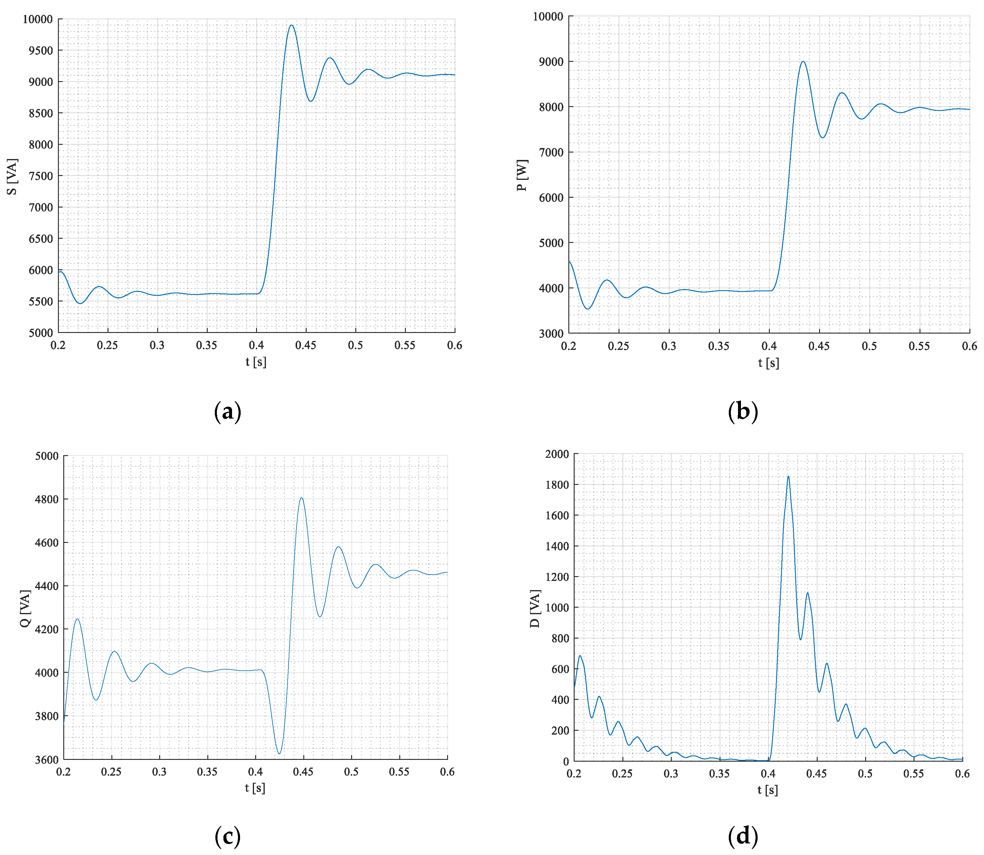
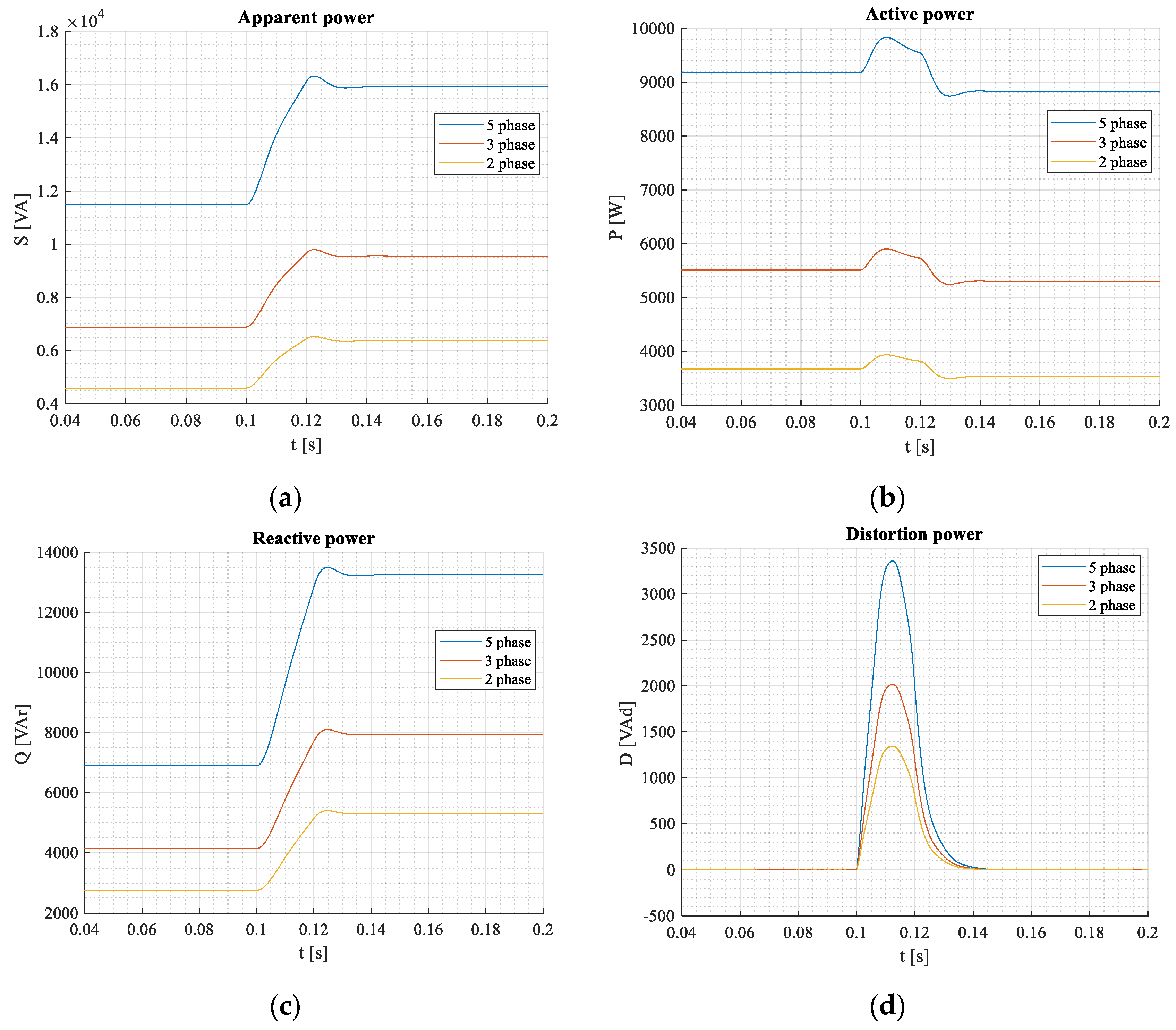
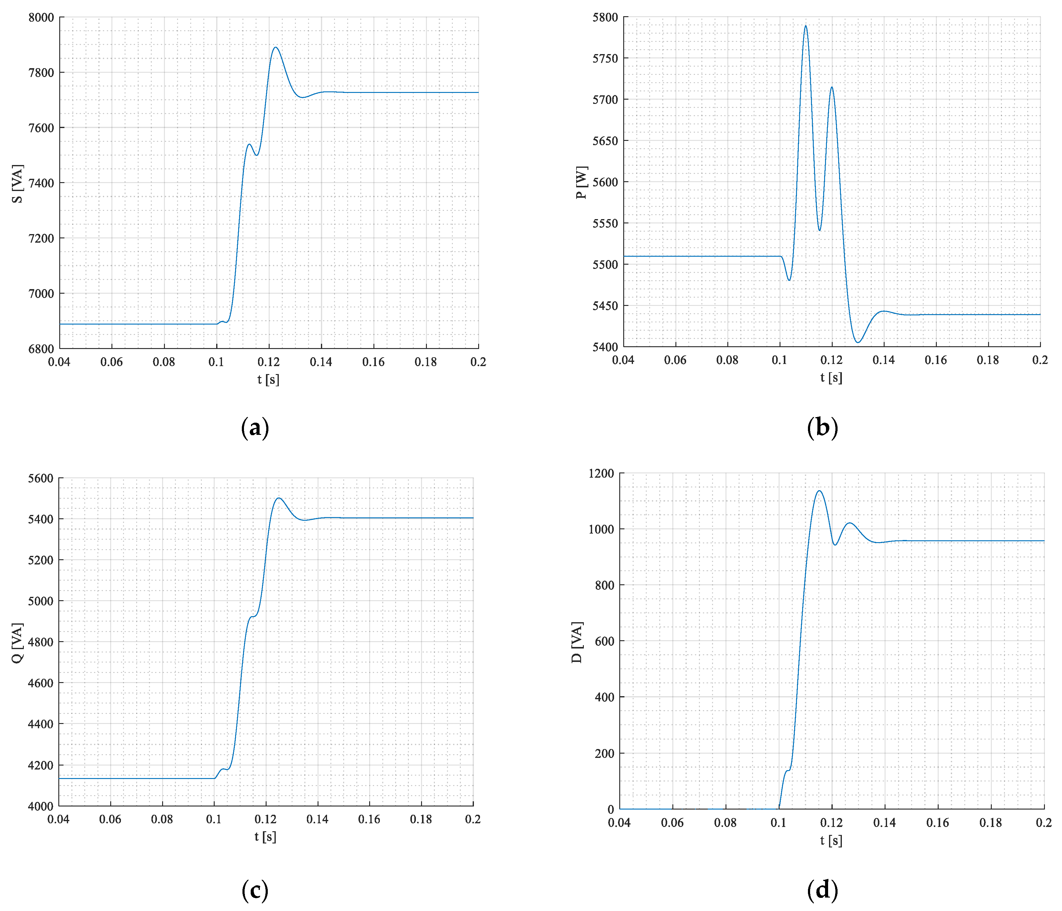
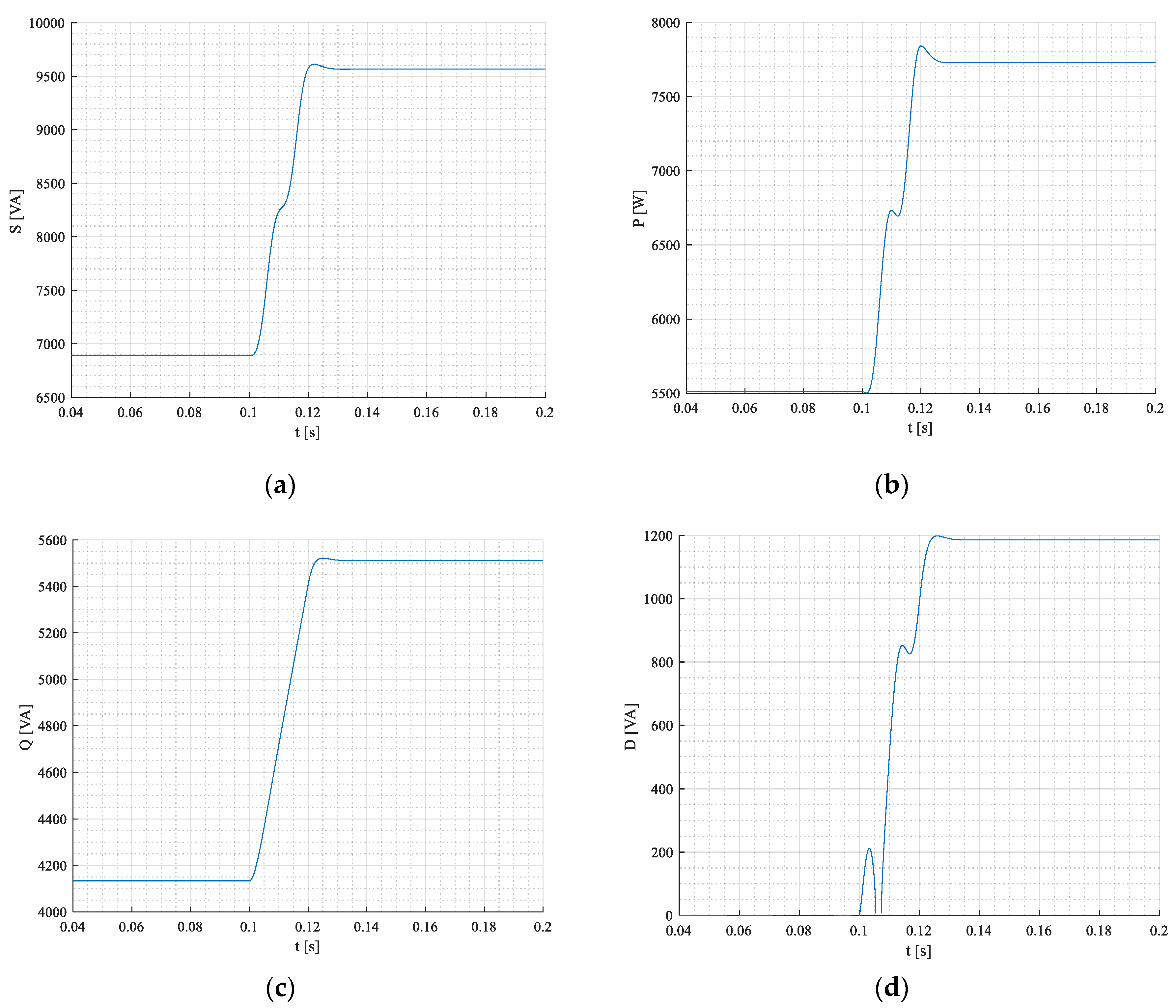
Figure 8.
Apparent—(a), active—(b), blind—(c), and distortion (d) power components during transient states of induction motor.
Figure 8.
Apparent—(a), active—(b), blind—(c), and distortion (d) power components during transient states of induction motor.
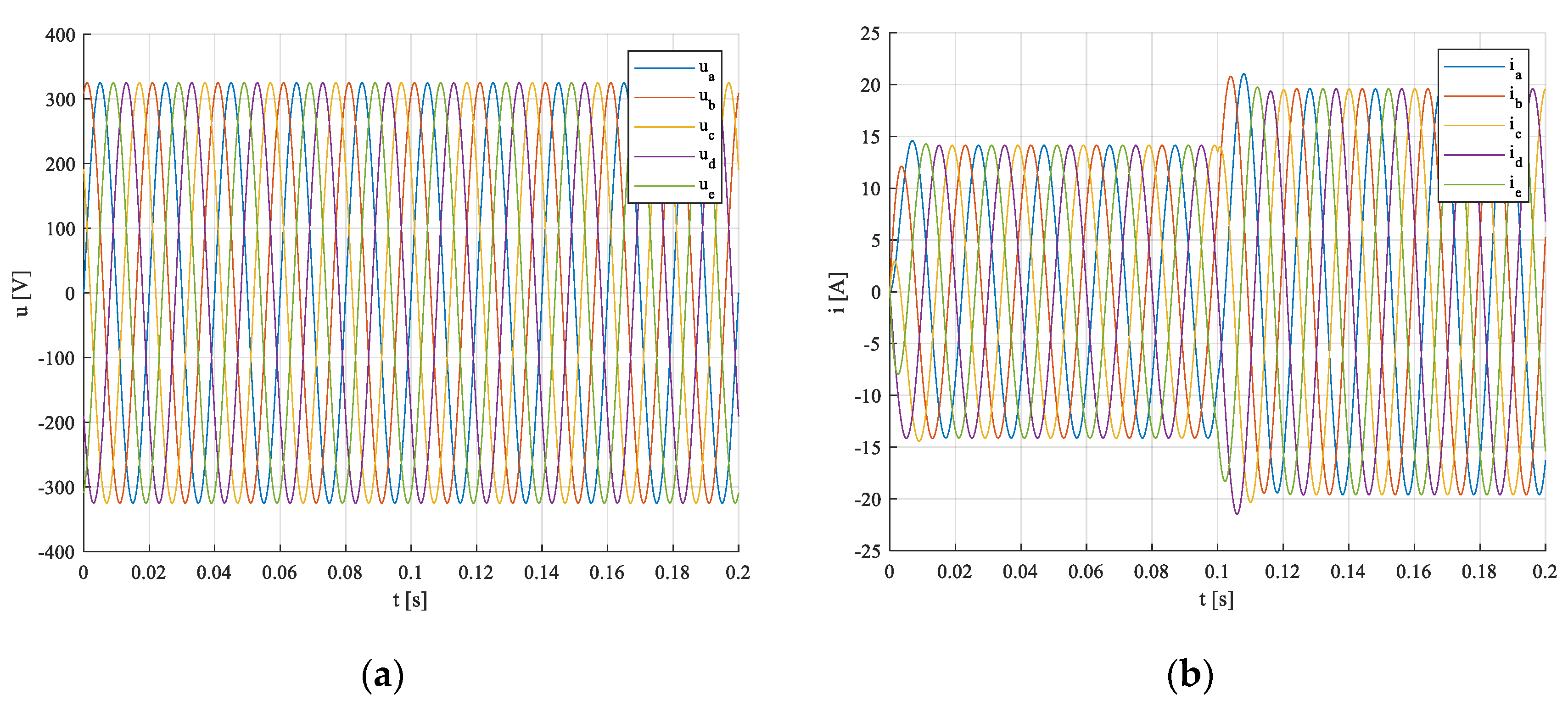
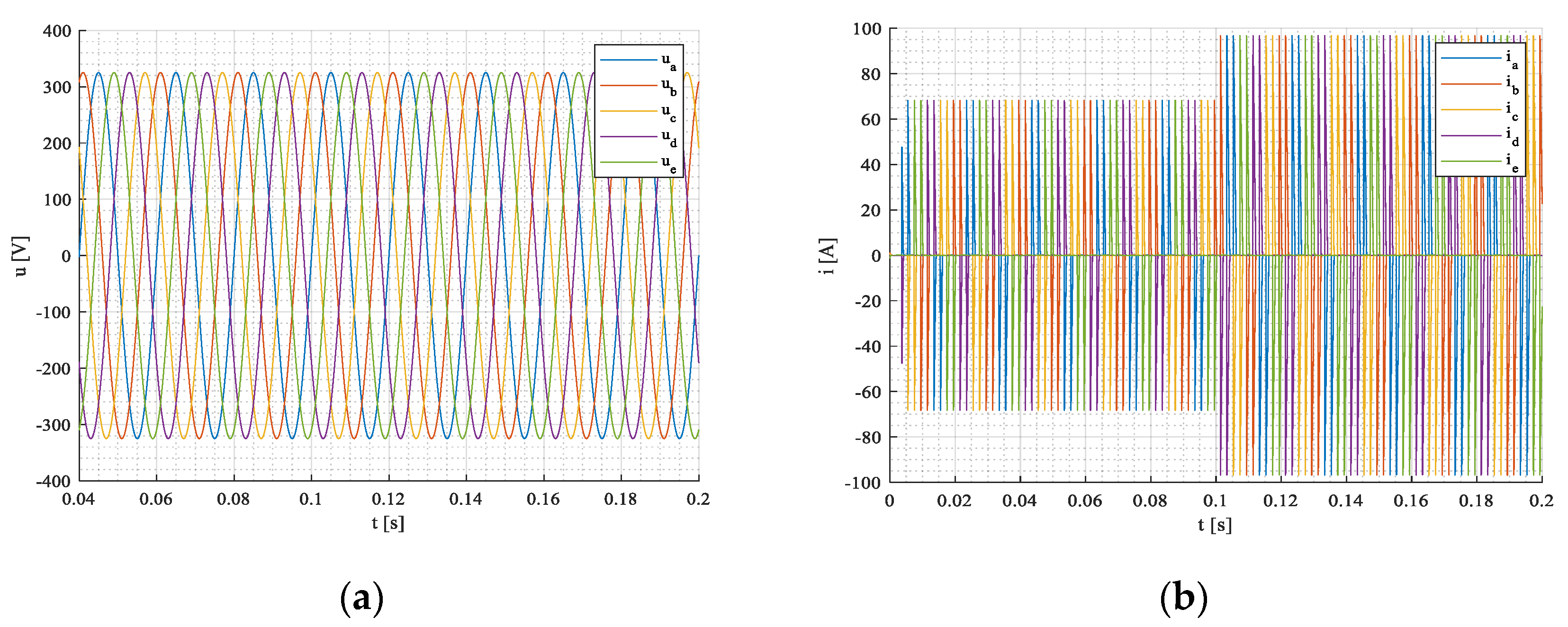
Figure 9.
Phase voltages (a) and currents (b) in —coordinates.
Figure 9.
Phase voltages (a) and currents (b) in —coordinates.
Figure 10.
Phase voltages (a) and load currents (b) in coordinates.
Figure 10.
Phase voltages (a) and load currents (b) in coordinates.
Figure 11.
Apparent (a), active (b), blind (c), and distortion (d) power components during transient states for 3-, 5-, and 2-phase systems under mains supplied linear RL load.
Figure 11.
Apparent (a), active (b), blind (c), and distortion (d) power components during transient states for 3-, 5-, and 2-phase systems under mains supplied linear RL load.
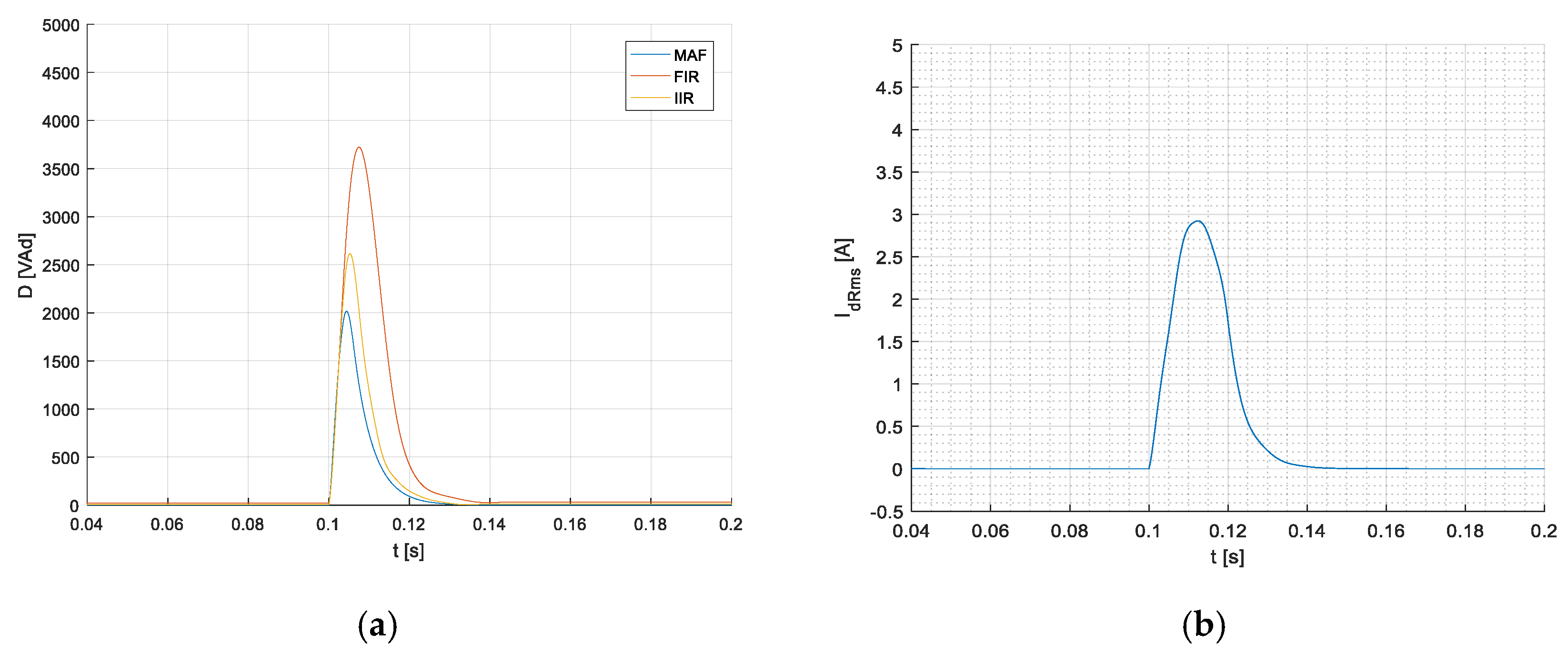
Figure 12.
Waveforms of distortion power components during transient states calculated by different methods (MAF-, DFIR, and DIIR filters) (a), and the corresponding deformation component of the current using the MAF method (b).
Figure 12.
Waveforms of distortion power components during transient states calculated by different methods (MAF-, DFIR, and DIIR filters) (a), and the corresponding deformation component of the current using the MAF method (b).
Figure 13.
The basic scheme of the considered systems: 3-phase (a), 5-phase (b), and 2-phase (c).
Figure 13.
The basic scheme of the considered systems: 3-phase (a), 5-phase (b), and 2-phase (c).
Figure 14.
Network voltages (a) and currents (b) in - coordinate systems.
Figure 14.
Network voltages (a) and currents (b) in - coordinate systems.
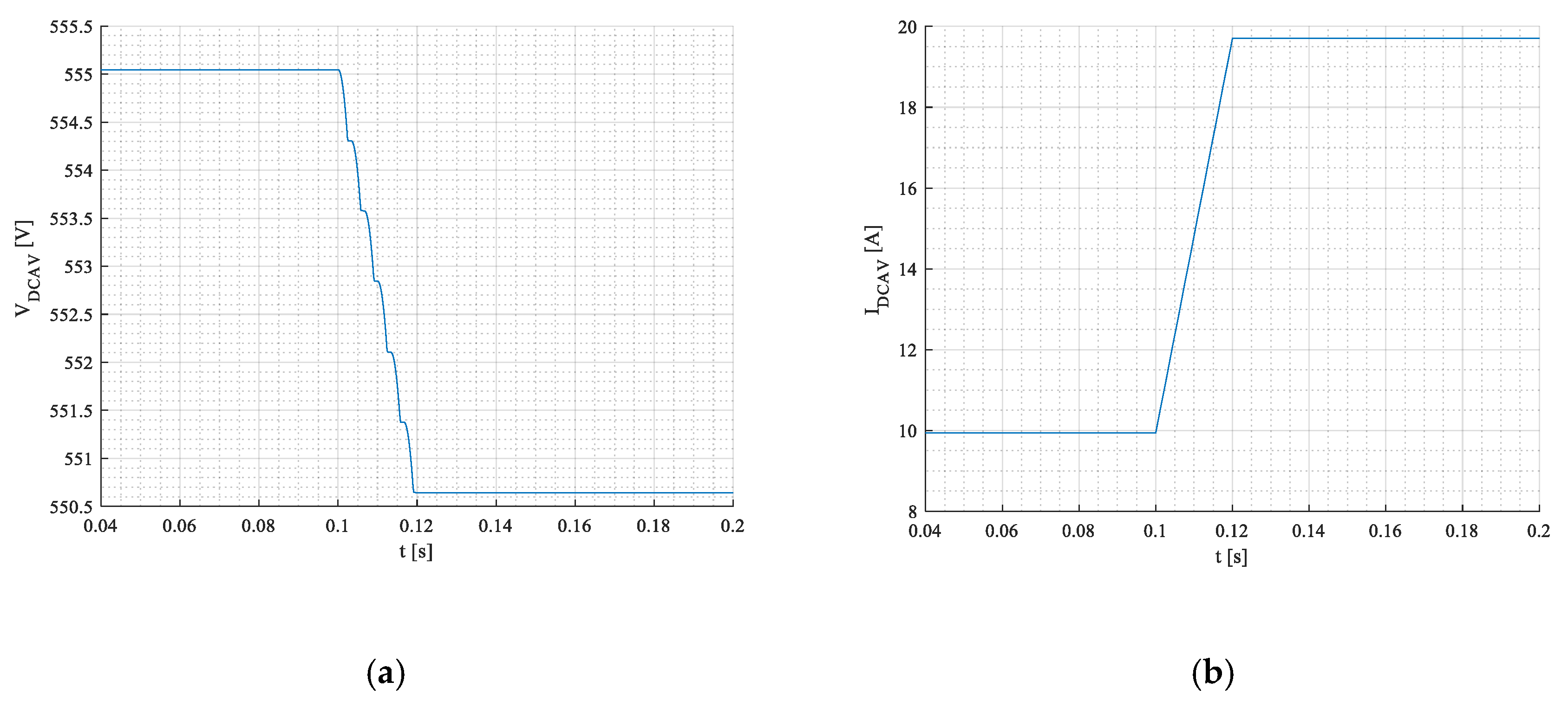
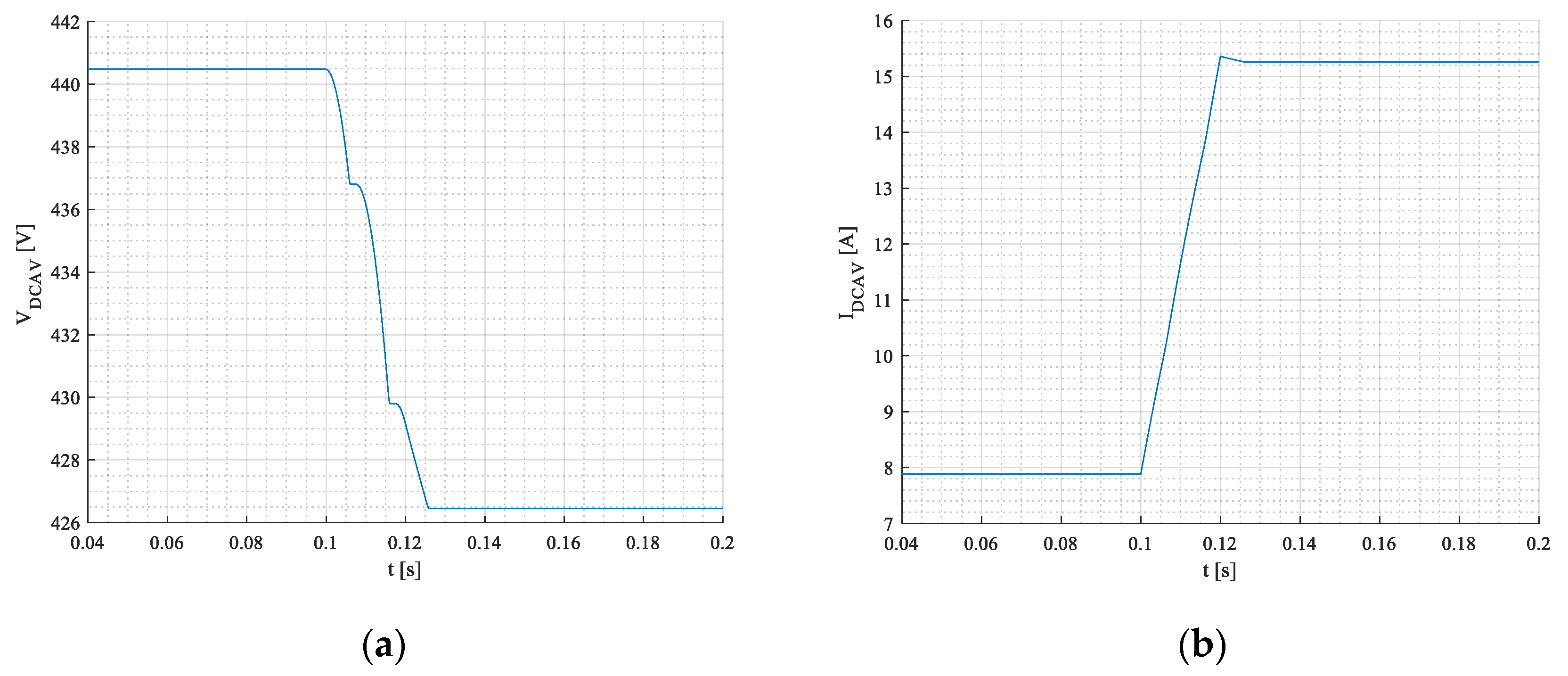
Figure 15.
Voltage (a) and current (b) on the DC side of a rectifier, under step change of resistive load.
Figure 15.
Voltage (a) and current (b) on the DC side of a rectifier, under step change of resistive load.
Figure 16.
Phase voltages (a), currents (b) in - coordinate system during transient.
Figure 16.
Phase voltages (a), currents (b) in - coordinate system during transient.
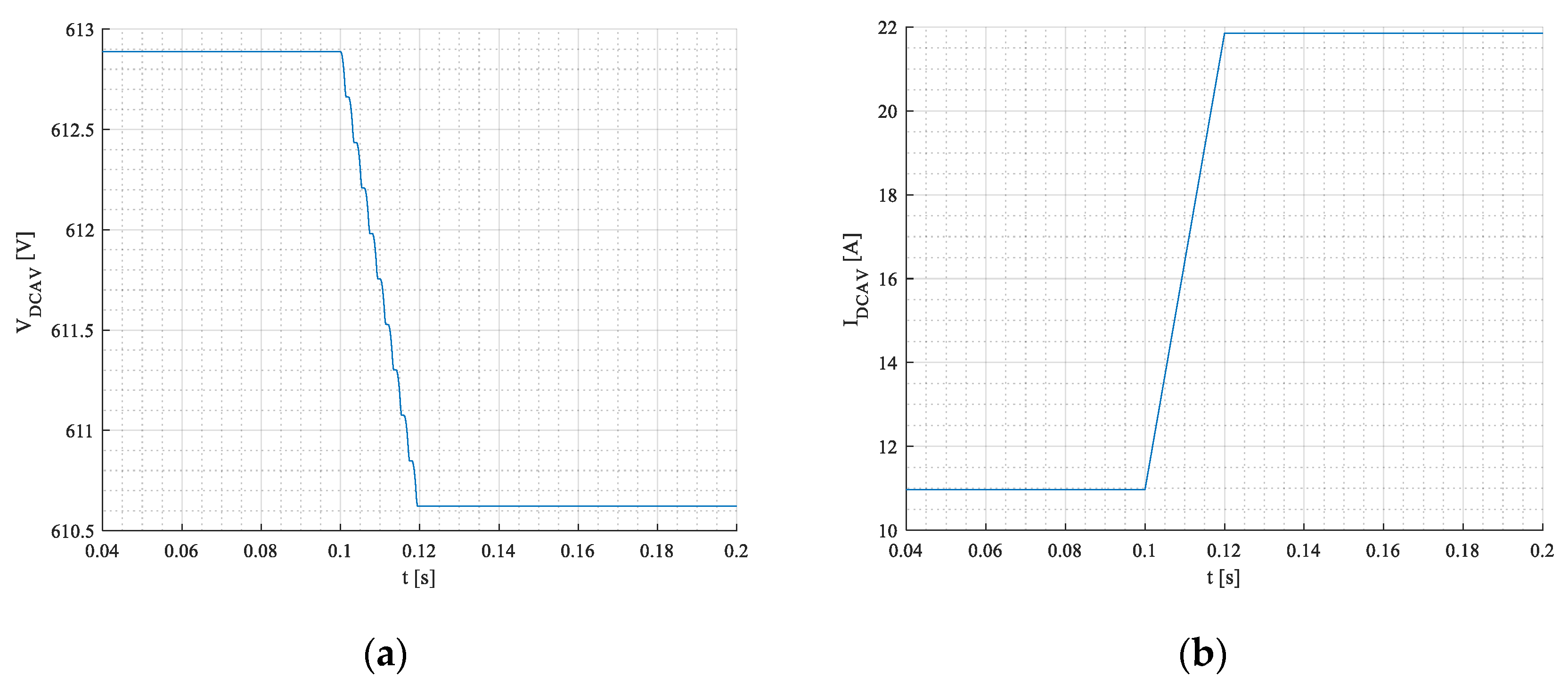
Figure 17.
Voltage (a) and current (b) in the DC side under step change of resistive load.
Figure 17.
Voltage (a) and current (b) in the DC side under step change of resistive load.
Figure 18.
Phase voltages (a), currents in (b) during transient.
Figure 18.
Phase voltages (a), currents in (b) during transient.
Figure 19.
Voltage (a) and current (b) on the DC side under resistive load.
Figure 19.
Voltage (a) and current (b) on the DC side under resistive load.
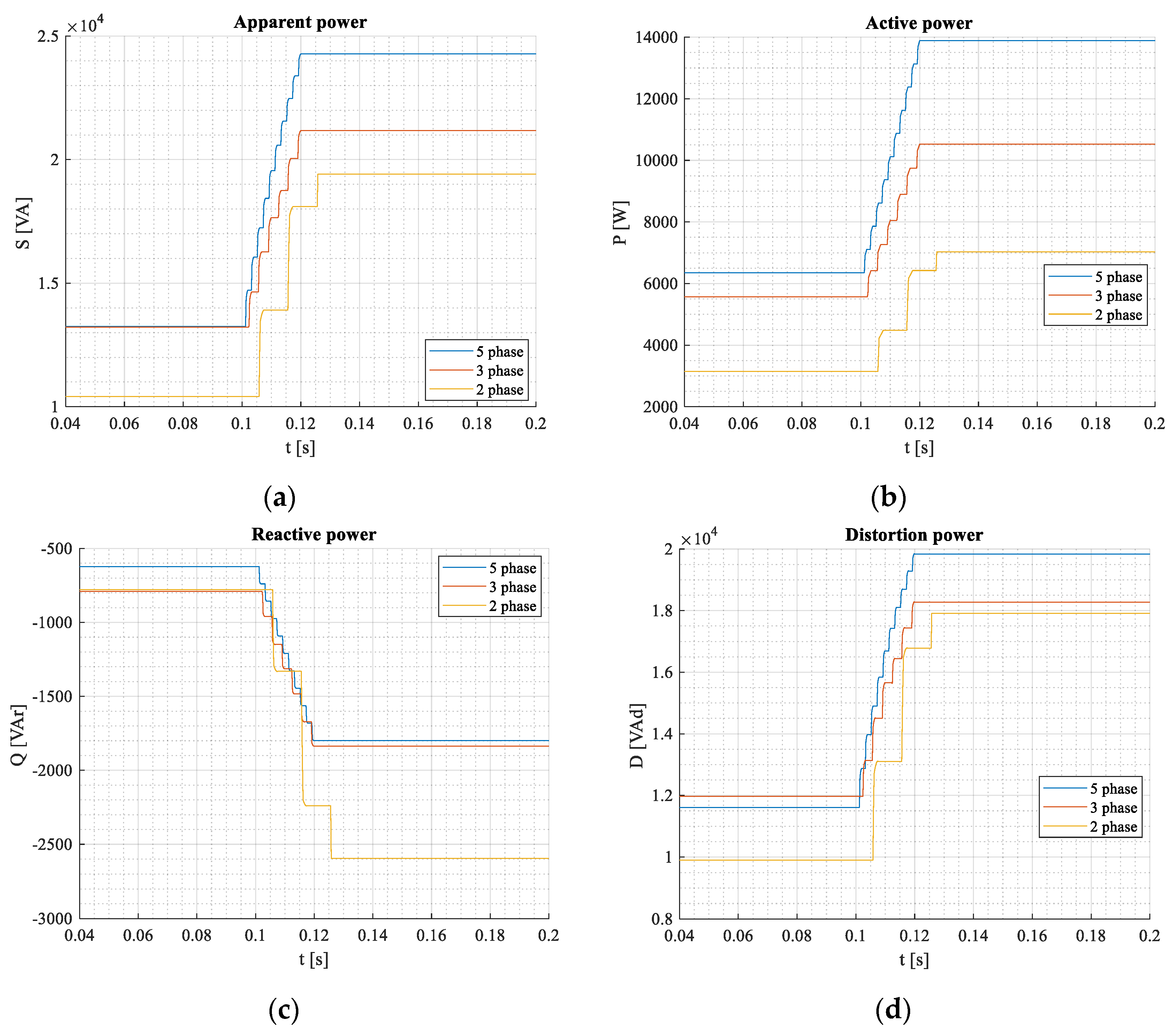
Figure 20.
Apparent—(a), active—(b), blind—(c), and distortion (d) power components during transient states for 3-, 5-, and 2-phase systems under mains supplied rectifier load.
Figure 20.
Apparent—(a), active—(b), blind—(c), and distortion (d) power components during transient states for 3-, 5-, and 2-phase systems under mains supplied rectifier load.
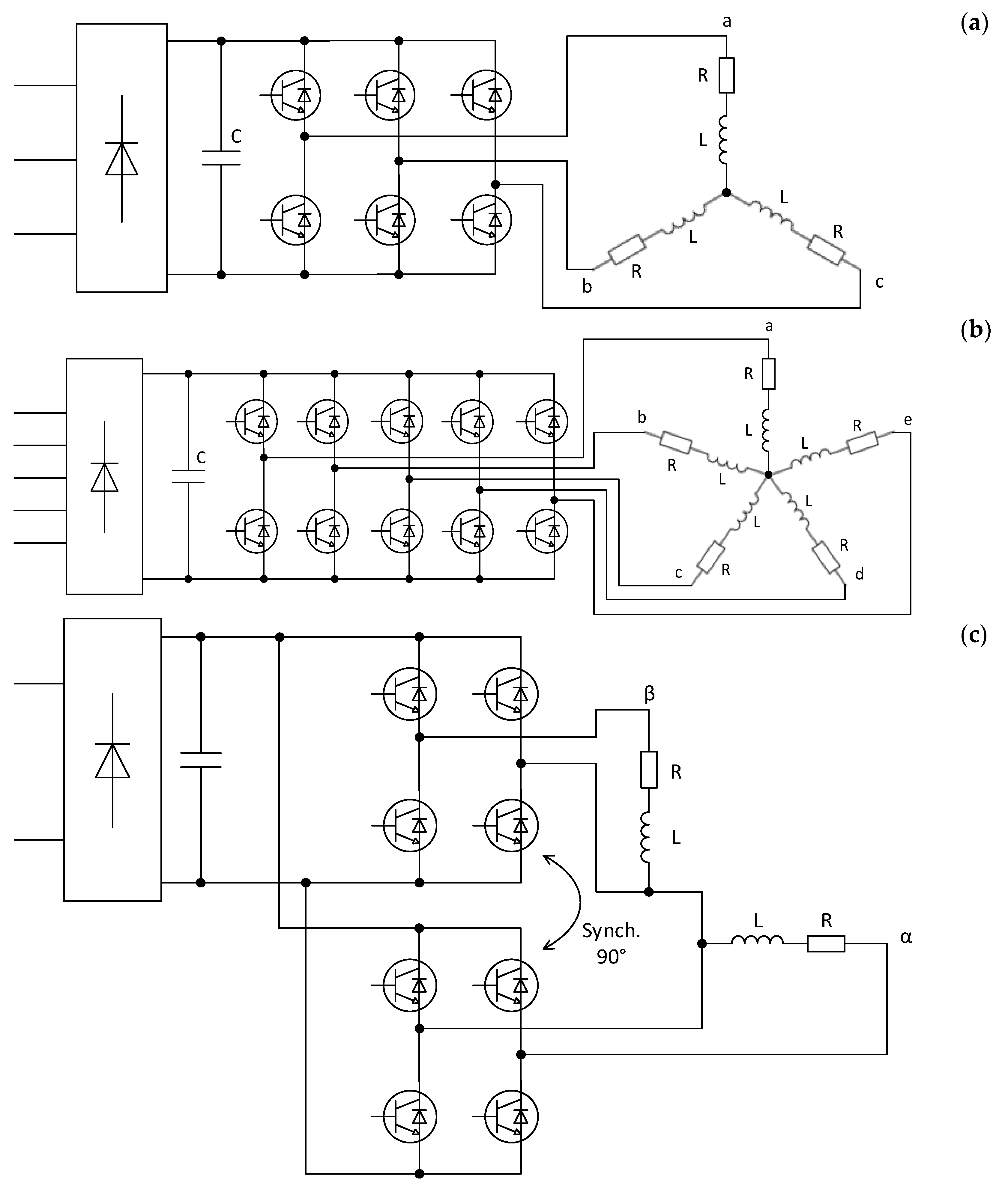
Figure 21.
The basic scheme of the considered systems: 3-phase (a), 5-phase (b), and 2-phase (c).
Figure 21.
The basic scheme of the considered systems: 3-phase (a), 5-phase (b), and 2-phase (c).
Figure 22.
VSI inverter voltages (a) and currents (b) in —coordinate system during the transient.
Figure 22.
VSI inverter voltages (a) and currents (b) in —coordinate system during the transient.
Figure 23.
VSI inverter voltages (a) and currents (b) in - coordinate system during the transient.
Figure 23.
VSI inverter voltages (a) and currents (b) in - coordinate system during the transient.
Figure 24.
VSI inverter voltages (a) and currents (b) inresp. in - systems during the transient.
Figure 24.
VSI inverter voltages (a) and currents (b) inresp. in - systems during the transient.
Figure 25.
Apparent—(a), active—(b), blind—(c), and distortion (d) power components during transient states for 3-, 5-, and 2-phase systems under inverter-supplied linear RL load.
Figure 25.
Apparent—(a), active—(b), blind—(c), and distortion (d) power components during transient states for 3-, 5-, and 2-phase systems under inverter-supplied linear RL load.
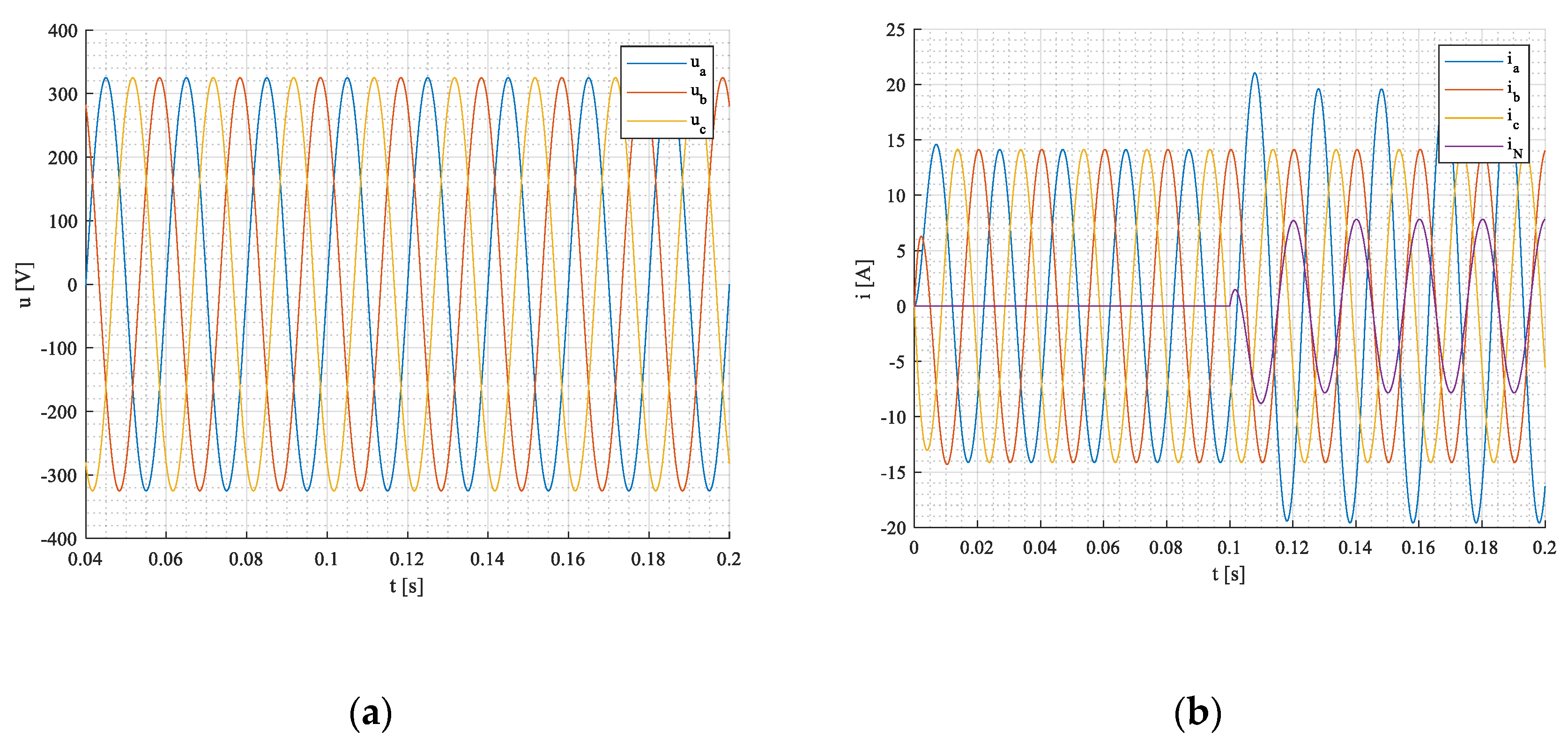
Figure 26.
Network voltages (a), load, and neutral currents (b).
Figure 26.
Network voltages (a), load, and neutral currents (b).
Figure 27.
Apparent-(a), active-(b), blind-(c), and distortion (d) power components during transient states for 3-phase system under a symmetrical network supplying non-symmetrical linear RL load.
Figure 27.
Apparent-(a), active-(b), blind-(c), and distortion (d) power components during transient states for 3-phase system under a symmetrical network supplying non-symmetrical linear RL load.
Figure 28.
Network voltages (a), load, and neutral currents (b).
Figure 28.
Network voltages (a), load, and neutral currents (b).
Figure 29.
Apparent- (a), active-(b), blind-(c), and distortion (d)power components during transient states for the 3-phase system under inverter-supplied non-symmetrical linear RL load.
Figure 29.
Apparent- (a), active-(b), blind-(c), and distortion (d)power components during transient states for the 3-phase system under inverter-supplied non-symmetrical linear RL load.
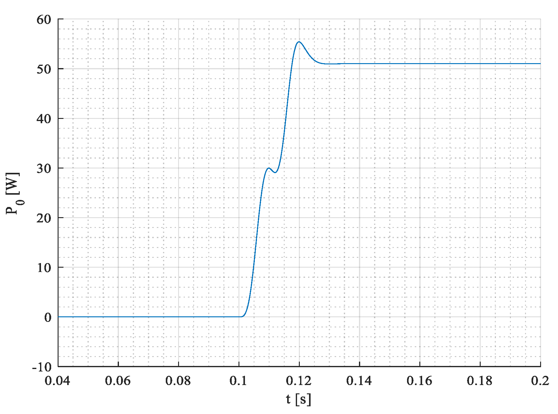
Figure 30.
The waveform of zero power component Po.
Figure 30.
The waveform of zero power component Po.
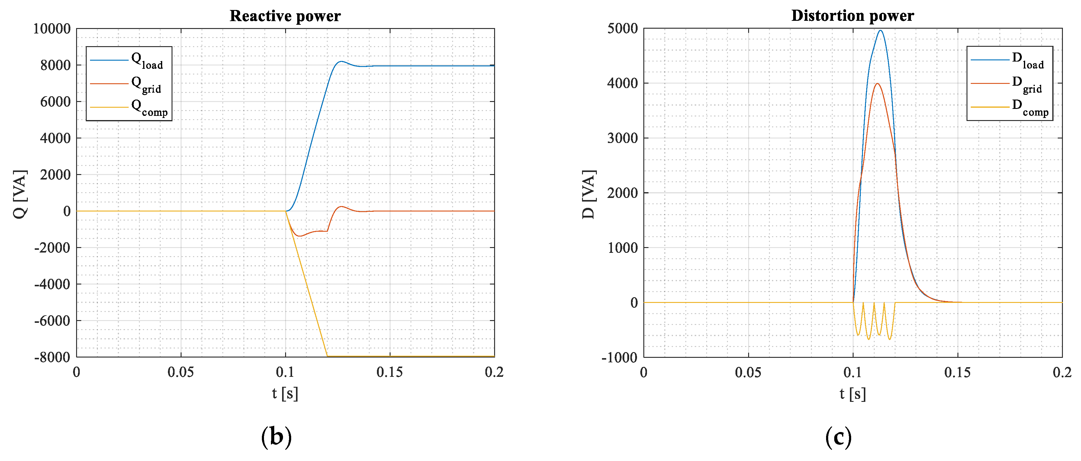
Figure 31.
Using switched capacitors (a) for compensating reactive blind power (b) under linear RL load and distortion power (c).
Figure 31.
Using switched capacitors (a) for compensating reactive blind power (b) under linear RL load and distortion power (c).
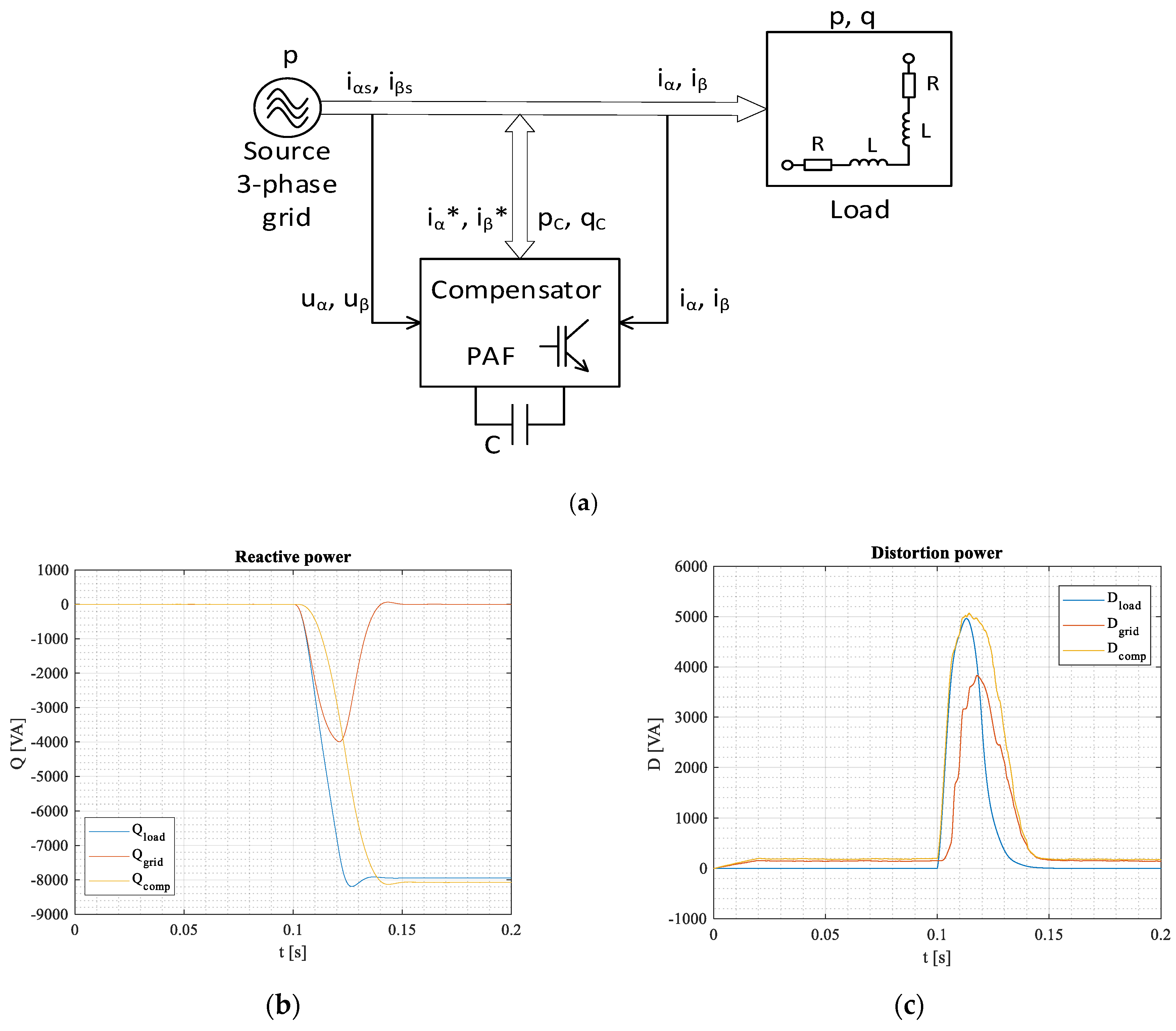
Figure 32.
Using PAF active filter (a) for compensating reactive blind power (b) under linear RL load and distortion power (c).
Figure 32.
Using PAF active filter (a) for compensating reactive blind power (b) under linear RL load and distortion power (c).
Table 1.
Load parameters for steady states before and after load change.
Table 1.
Load parameters for steady states before and after load change.
| Load | | | | | | | |
|---|
| before | | | | | | | |
| after | | | | | | | |
Table 2.
Classical calculation before and after the change (at steady states).
Table 2.
Classical calculation before and after the change (at steady states).
| Time | | | | | | | |
|---|
| | | | | | | |
| | | | | | | |
Table 3.
Simulation results before and after the change (at steady states).
Table 3.
Simulation results before and after the change (at steady states).
| Time | | | | | | | |
|---|
| t = 0.1 s | 229.8 | 229.8 | 9.991 | 9.991 | 14.13 | 36.88 | 0.7947 |
| t = 0.2 s | 229.8 | 229.8 | 13.85 | 13.85 | 19.60 | 56.31 | 0.5547 |
Table 4.
Simulation results before and after the change (at steady states).
Table 4.
Simulation results before and after the change (at steady states).
| Time | | | | | | | |
|---|
| t = 0.1 s | 6888.5 | 5510.6 | 4133.3 | 0 | 0.7999 | 0 | 0 |
| t = 0.2 s | 9551.5 | 5298.9 | 7946.9 | 0 | 0.5547 | 0 | 0 |
Table 5.
IM motor parameters for steady-state before and after load change.
Table 5.
IM motor parameters for steady-state before and after load change.
| Load | | | | | | | |
|---|
| before | | | | | | | |
| after | | | | | | | |
Table 6.
Simulation results before and after the change (at steady states).
Table 6.
Simulation results before and after the change (at steady states).
| Time | | | | | | | |
|---|
| | | 8.145 | 8.148 | 11.52 | 45.66 | 0.70 |
| | | 13.21 | 13.22 | 18.69 | 29.30 | 0.87 |
Table 7.
Simulation results before and after the change (at steady states).
Table 7.
Simulation results before and after the change (at steady states).
| Time | | | | | | | | |
|---|
| 5.616 | 3.932 | 4.010 | 4.566 | 0.70 | | 3.932 | |
| 9.109 | 7.937 | 4.459 | 12.27 | 0.87 | | 7.936 | |
Table 8.
Load parameters for steady states before and after load change.
Table 8.
Load parameters for steady states before and after load change.
| Load | | | | | | | |
|---|
| before | | | | | | | |
| after | | | | | | | |
Table 9.
Classical calculation before and after the change (at steady states).
Table 9.
Classical calculation before and after the change (at steady states).
| Time | | | | | | | |
|---|
| | | | | | | |
| | | | | | | |
Table 10.
Simulation results before and after the change (at steady states).
Table 10.
Simulation results before and after the change (at steady states).
| Time | | | | | | | |
|---|
| | | | | | | |
| | | | | | | |
Table 11.
Simulation results before and after the change (at steady states).
Table 11.
Simulation results before and after the change (at steady states).
| Time | | | | | | | | |
|---|
| | | | | | | | |
| | | | | | | | |
Table 12.
Load parameters for steady states before and after load change.
Table 12.
Load parameters for steady states before and after load change.
| Load | | | | | | | |
|---|
| before | | | | | | | |
| after | | | | | | | |
Table 13.
Classical calculation before and after the change (at steady states).
Table 13.
Classical calculation before and after the change (at steady states).
| Time | | | | | | | |
|---|
| | | | | | | |
| | | | | | | |
Table 14.
Simulation results before and after the change (at steady states).
Table 14.
Simulation results before and after the change (at steady states).
| Time | | | | | | | |
|---|
| | | | | | | |
| | | | | | | |
Table 15.
Simulation results before and after the change (at steady states).
Table 15.
Simulation results before and after the change (at steady states).
| Time | | | | | | | | |
|---|
| | | | | | | | |
| | | | | | | | |
Table 16.
Load parameters for steady states before and after load change.
Table 16.
Load parameters for steady states before and after load change.
| Load | | |
|---|
| before | | |
| after | | |
Table 17.
Simulation results before and after the change (at steady states).
Table 17.
Simulation results before and after the change (at steady states).
| Time | | | | | | | |
|---|
| | | | | | | |
| | | | | | | |
Table 18.
Simulation results before and after the change (at steady states).
Table 18.
Simulation results before and after the change (at steady states).
| Time | | | | | | | | |
|---|
| | | | | | | | |
| | | | | | | | |
Table 19.
Load parameters for steady states before and after load change.
Table 19.
Load parameters for steady states before and after load change.
| Load | | |
|---|
| before | | |
| after | | |
Table 20.
Simulation results before and after the change (at steady states).
Table 20.
Simulation results before and after the change (at steady states).
| Time | | | | | | | |
|---|
| | | | | | | |
| | | | | | | |
Table 21.
Simulation results before and after the change (at steady states).
Table 21.
Simulation results before and after the change (at steady states).
| Time | | | | | | | | |
|---|
| | | | | | | | |
| | | | | | | | |
Table 22.
Load parameters for steady states before and after load change.
Table 22.
Load parameters for steady states before and after load change.
| Load | | |
|---|
| before | | |
| after | | |
Table 23.
Simulation results before and after the change (at steady states).
Table 23.
Simulation results before and after the change (at steady states).
| Time | | | | | | | |
|---|
| | | | | | | |
| | | | | | | |
Table 24.
Simulation results before and after the change (at steady states).
Table 24.
Simulation results before and after the change (at steady states).
| Time | | | | | | | | |
|---|
| | | | | | | | |
| | | | | | | | |
Table 25.
Load parameters for steady states before and after load change.
Table 25.
Load parameters for steady states before and after load change.
| Load | | | | | | | |
|---|
| before | | | | | | | |
| after | | | | | | | |
Table 26.
Classical calculation before and after the change (at steady states).
Table 26.
Classical calculation before and after the change (at steady states).
| Time | | | | | | | |
|---|
| | | | | | | |
| | | | | | | |
Table 27.
Simulation results before and after the change (at steady states).
Table 27.
Simulation results before and after the change (at steady states).
| Time | | | | | | | |
|---|
| | | | | | | |
| | | | | | | |
Table 28.
Simulation results before and after the change (at steady states).
Table 28.
Simulation results before and after the change (at steady states).
| Time | | | | | | | | |
|---|
| | | | | | | | |
| | | | | | | | |
Table 29.
Load parameters for steady states before and after load change.
Table 29.
Load parameters for steady states before and after load change.
| Load | | | | | | | |
|---|
| before | | | | | | | |
| after | | | | | | | |
Table 30.
Classical calculation before and after the change (at steady states).
Table 30.
Classical calculation before and after the change (at steady states).
| Time | | | | | | | |
|---|
| | | | | | | |
| | | | | | | |
Table 31.
Simulation results before and after the change (at steady states).
Table 31.
Simulation results before and after the change (at steady states).
| Time | | | | | | | |
|---|
| | | | | | | |
| | | | | | | |
Table 32.
Simulation results before and after the change (at steady states).
Table 32.
Simulation results before and after the change (at steady states).
| Time | | | | | | | | |
|---|
| | | | | | | | |
| | | | | | | | |
Table 33.
Load parameters for steady states before and after load change.
Table 33.
Load parameters for steady states before and after load change.
| Load | | | | | | | |
|---|
| before | | | | | | | |
| after | | | | | | | |
Table 34.
Classical calculation before and after the change (at steady states).
Table 34.
Classical calculation before and after the change (at steady states).
| Time | | | | | | | |
|---|
| | | | | | | |
| | | | | | | |
Table 35.
Simulation results before and after the change (at steady states).
Table 35.
Simulation results before and after the change (at steady states).
| Time | | | | | | | |
|---|
| | | | | | | |
| | | | | | | |
Table 36.
Simulation results before and after the change (at steady states).
Table 36.
Simulation results before and after the change (at steady states).
| Time | | | | | | | | |
|---|
| | | | | | | | |
| | | | | | | | |
Table 37.
Load parameters for steady states before and after load change.
Table 37.
Load parameters for steady states before and after load change.
| Load | | | | | | | |
|---|
| before | | | | | | | |
| after | | | | | | | |
Table 38.
Simulation results before and after the change (at steady states).
Table 38.
Simulation results before and after the change (at steady states).
| Time | | | | | | |
|---|
| | | | | | |
| | | | | | |
Table 39.
Simulation results before and after the change (at steady states).
Table 39.
Simulation results before and after the change (at steady states).
| Time | | | | | | | |
|---|
| | | | | | | |
| | | | | | | |
Table 40.
Load parameters for steady states before and after load change.
Table 40.
Load parameters for steady states before and after load change.
| Load | | | | | | | |
|---|
| before | | | | | | | |
| after | | | | | | | |
Table 41.
Simulation results before and after the change (at steady states).
Table 41.
Simulation results before and after the change (at steady states).
| Time | | | | | | |
|---|
| | | | | | |
| | | | | | |
Table 42.
Simulation results before and after the change (at steady states).
Table 42.
Simulation results before and after the change (at steady states).
| Time | | | | | | | |
|---|
| | | | | | | |
| | | | | | | |


