Nash Equilibria of Quantum Games in the Special Two-Parameter Strategy Space

Abstract

The aim of the paper is to examine pure Nash equilibria in a quantum game that extends the classical bimatrix game of dimension 2. The strategies of quantum players are specific types of two-parameter unitary operations such that the resulting quantum game is invariant under isomorphic transformations of the input classical game. We formulate general statements for the existence and form of Nash equilibria and discuss their Pareto efficiency. We prove that, depending on the payoffs of a classical game, the corresponding quantum game may or may not have Nash equilibria in the set of unitary strategies under study. Some of the equilibria cease to be equilibria if the players’ strategy set is the three-parameter special unitary group.

1. Introduction

Game theory, which was initiated in 1928 by John von Neumann in the [1] and developed in [2], is one of the younger branches of mathematics. The aim of this theory is the mathematical modeling of participants’ behavior in conflict situations, generally assuming that they seek to maximize their profits. The theory of quantum games, developed on the border of game theory and quantum mechanics, is an extension of this theory. It is an interdisciplinary research area in which it is assumed that games and decision problems are played with the use of quantum objects. The non-classical properties of these objects are essential for the way the game is played and the result of the game.

The work widely recognized as the beginning of quantum game theory is [3]. D. Meyer showed on the example of a simple extensive game in which a player equipped with unitary strategies has a winning strategy. Among the other fundamental works on quantum game theory, the work [4] is of particular importance. The scheme introduced by J. Eisert, M. Wilkens and M. Lewenstein was the first formal protocol for playing a quantum game. The presented model uses the formalism of quantum computing for the description of any $2\times 2$ bimatrix game. According to the main assumptions of the scheme, the players’ strategies are unitary operations dependent on two parameters, and the players act with these operators on the maximal entangled two-qubit state.

An alternative model of the quantum playing of the bimatrix game is the scheme introduced by Marinatto and Weber in [5]. In this case, the players’ strategies were restricted to two unitary matrices (the identity and the Pauli matrix X), with the initial state being any fixed two-qubit state. Quantum game theory also includes quantum models for games with infinite sets of strategies. The work [6] presents a minimalist model for the quantum playing of the Cournot duopoly—a two person normal-form game, in which the set of strategies of each player is identified with the interval $[0,\infty )$. The theory of quantum games continues to develop dynamically, as evidenced by recent works [7,8,9,10].

The discussion on various parameterizations of unitary strategies has already started with the first scheme of quantum playing of the $2\times 2$ game [4]. The authors defined a quantum approach to the prisoner’s dilemma game. In this quantum game, the set of strategies of both players was a two-parameter subset of unitary operators from $\mathsf{SU}(2)$. The quantum game defined in this way was characterized by a unique and pareto-optimal Nash equilibrium. It turned out that the unique result of the game presented in the paper [4] is closely related to the choice of the set of unitary strategies available to the players. In the comment [11], it was shown that the quantum prisoner’s dilemma does not have the pareto-optimal Nash equilibrium if the sets of players’ strategies are equal to full $\mathsf{SU}(2)$. Moreover, in such a case, there is not even a Nash equilibrium in pure strategies. The stability predicted by the equilibrium is only obtained when the players choose their strategies according to a certain probability distribution [11,12,13].

In the paper [14], other types of two-parameter strategies were considered, and their significant influences on the final result of the game, in particular, on the form of Nash equilibrium, were discussed. However, the dominant trend in the literature on the EWL scheme was the free use of various types of two-parameter strategies [15,16,17,18,19]. The works [20,21] attempted to answer the question of what types of sets of unitary operations are appropriate in the EWL game. For this purpose, it was examined whether pairs of classical isomorphic games remain isomorphic when played in the quantum way. One of the main results of the paper [20] was to show that the application of the EWL scheme and certain types of unitary two-parameter operations to a pair of isomorphic games may imply different sets of Nash equilibria for a pair of isomorphic games. In particular, in the game examined in [4], the swapping of the columns of the classical bimatrix game made the pareto-optimal Nash equilibrium in the quantum game no longer achievable. Moreover, it was shown in [20] that the isomorphism of quantum games occurs when the sets of players’ strategies are extended to $\mathsf{SU}(2)$. Paper [21] presents a specific type of two-parameter unitary operation that meets the isomorphism criterion in the same way as $\mathsf{SU}(2)$. The result is important because EWL with such strategies allows one to find Nash equilibria in pure strategies in many non-trivial games, which is not the case with $\mathsf{SU}(2)$.

The aim of the present paper is to investigate pure strategies Nash equilibria of $2\times 2$ bimatrix games in the parametrization introduced in [21]. The example considered in [21] shows the existence of Nash equilibria in games where players do not have convergent preferences about the payoff vectors. Thus, it seems extremely interesting to point out general classes of games with Nash equilibria in this parametrization. In the present paper, we formulate general conditions that guarantee the Nash equilibrium. We also point out some special classes of games that do not have the equilibrium.

In Section 2, we briefly recall the definition of a quantum game in the EWL scheme and a 2-dimensional parameterization of players’ strategies that is invariant under isomorphic transformations of the input game. We introduce two payoff functions: one which is based on the classical payoff matrix and the other which is based on the symmetrized payoffs. In Section 3, we investigate the existence of Nash equilibria for the game and prove two propositions. The first proposition refers to Nash equilibria when odd symmetrized payoffs, both diagonal and antidiagonal, are of the same sign for both players. The second proposition shows the existence of Nash equilibria for games that have a dominant pair of players’ payoffs in their classical form. In Section 4, we show two game classes that do not have Nash equilibria in the parameterization studied. Proposition 3 shows this for the prisoner’s dilemma and the game of chicken, whereas Proposition 4 shows this for the battle of the sexes. We summarize the results in Section 5.

2. The Eisert–Wilkens–Lewenstein (EWL) Scheme

In this section, we briefly review the quantum game scheme based on the idea of J. Eisert, M. Wilkens and M. Lewenstein [4] in its generalized form similar to [14]. The EWL scheme concerns $2\times 2$ bimatrix games. A $2\times 2$ bimatrix game is a two-player game with two strategies for each player. It can be described by a matrix

$$(A,B)=\left(\begin{array}{cc}(a_{00},b_{00})& (a_{01},b_{01})\\ (a_{10},b_{10})& (a_{11},b_{11})\end{array}\right).$$

(1)

The first player’s strategies are identified with the rows and the second player’s with the columns. If the first player chooses row k and the second player chooses column l, their resulting payoffs are $a_{kl}$ and $b_{kl}$, respectively. We consider the Eisert–Wilkens–Lewenstein approach to the game (1) defined by a triple

$$(N,{(D_p)}_{p\in N},{({\Pi }_p)}_{p\in N}),$$

(2)

where

• $N=\{a,b\}$ is the set of players;
• $D_p=\left\{({\theta }_p,{\varphi }_p):{\theta }_p\in [0,\pi ]\mathrm{and}{\varphi }_p\in [0,2\pi )\right\}$; $p\in \{a,b\}$, are sets of players’ strategies that define 2-parameter unitary operators

  $$U({\theta }_p,{\varphi }_p)=\left(\begin{array}{cc}{e}^{-i{\varphi }_p/2}cos\frac{{\theta }_p}{2}& -e^{-i{\varphi }_p/2}sin\frac{{\theta }_p}{2}\\ e^{i{\varphi }_p/2}sin\frac{{\theta }_p}{2}& e^{i{\varphi }_p/2}cos\frac{{\theta }_p}{2}\end{array}\right)\in \mathsf{SU}(2);$$

  (3)
• ${\Pi }_p:D_a\times D_b\to \mathbb{R}$ are the players’ quantum payoff functions given by

  $$\begin{array}{cc}\hfill & {\Pi }_a({\theta }_a,{\varphi }_a,{\theta }_b,{\varphi }_b)=\sum _{k,l=0}^1{P}_{k,l}({\theta }_a,{\varphi }_a,{\theta }_b,{\varphi }_b)a_{kl},\hfill \end{array}$$

  (4)

  $$\begin{array}{cc}\hfill & {\Pi }_b({\theta }_a,{\varphi }_a,{\theta }_b,{\varphi }_b)=\sum _{k,l=0}^1{P}_{k,l}({\theta }_a,{\varphi }_a,{\theta }_b,{\varphi }_b)b_{kl},\hfill \end{array}$$

  (5)

  where $a_{kl}$ and $b_{kl}$, $k,l\in \{0,1\}$, are the payoffs of the initial game (1) and

  $$\begin{array}{c}{P}_{0,0}({\theta }_a,{\varphi }_a,{\theta }_b,{\varphi }_b)={\left(cos\frac{{\theta }_a}{2}cos\frac{{\theta }_b}{2}cos\left(\frac{{\varphi }_a+{\varphi }_b}{2}\right)+sin\frac{{\theta }_a}{2}sin\frac{{\theta }_b}{2}sin\left(\frac{{\varphi }_a+{\varphi }_b}{2}\right)\right)}^2,\hfill \\ P_{0,1}({\theta }_a,{\varphi }_a,{\theta }_b,{\varphi }_b)={\left(cos\frac{{\theta }_a}{2}sin\frac{{\theta }_b}{2}cos\left(\frac{{\varphi }_a-{\varphi }_b}{2}\right)-sin\frac{{\theta }_a}{2}cos\frac{{\theta }_b}{2}sin\left(\frac{{\varphi }_a-{\varphi }_b}{2}\right)\right)}^2,\hfill \\ P_{1,0}({\theta }_a,{\varphi }_a,{\theta }_b,{\varphi }_b)={\left(cos\frac{{\theta }_a}{2}sin\frac{{\theta }_b}{2}sin\left(\frac{{\varphi }_a-{\varphi }_b}{2}\right)+sin\frac{{\theta }_a}{2}cos\frac{{\theta }_b}{2}cos\left(\frac{{\varphi }_a-{\varphi }_b}{2}\right)\right)}^2,\hfill \\ P_{1,1}({\theta }_a,{\varphi }_a,{\theta }_b,{\varphi }_b)={\left(cos\frac{{\theta }_a}{2}cos\frac{{\theta }_b}{2}sin\left(\frac{{\varphi }_a+{\varphi }_b}{2}\right)-sin\frac{{\theta }_a}{2}sin\frac{{\theta }_b}{2}cos\left(\frac{{\varphi }_a+{\varphi }_b}{2}\right)\right)}^2.\hfill \end{array}$$

  (6)

The coefficients $P_{k,l}({\theta }_a,{\varphi }_a,{\theta }_b,{\varphi }_b)\in [0,1]$ are probabilities depending on the players’ strategies (3) and can be derived from [14]

$$P_{k,l}({\theta }_a,{\varphi }_a,{\theta }_b,{\varphi }_b)={\left|⟨kl\left|J^{†}\left(U({\theta }_a,{\varphi }_a)\otimes U({\theta }_b,{\varphi }_b)\right)J\right|00⟩\right|}^2,$$

(7)

where $J=\frac{1}{\sqrt{2}}I\otimes I+\frac{i}{\sqrt{2}}{\sigma }_x\otimes {\sigma }_x$ is an entangling operator. As all transformations in (7) are unitary, the coefficients must be normalized

$$\sum _{k,l=0}^1{P}_{k,l}({\theta }_a,{\varphi }_a,{\theta }_b,{\varphi }_b)=1,{\theta }_a,{\theta }_b\in [0,\pi ]\mathrm{and}{\varphi }_a,{\varphi }_a\in [0,2\pi ).$$

(8)

Quantization (2) in parameterization (3) has an essential feature: that it is invariant under isomorphic transformations of the input classical game [20]. If the two classical games are strongly isomorphic, e.g., they differ in the order of players or the order of their strategies, then the corresponding quantum extensions should also be strongly isomorphic. The invariance criterion is crucial for the quantum game to be a true extension of the classical game. If this condition is not met, two isomorphic forms of the classical game can lead to non-equivalent quantum extensions. Then. it is not clear which of them should be considered as an extension of the classical game. This problem occurs when, for example, we use the parameterization of unitary operators studied in [4]:

$$U(\theta ,\varphi )=\left(\begin{array}{cc}{e}^{i\varphi }cos\frac{\theta }{2}& sin\frac{\theta }{2}\\ -sin\frac{\theta }{2}& e^{-i\varphi }cos\frac{\theta }{2}\end{array}\right).$$

(9)

Then two bimatrix games that differ in the order of the strategy of one player imply different quantum games [20]. The parameterization by the group $\mathsf{SU}(2)$ is also invariant under isomorphic transformations of the input game [20], but it allows for the existence of Nash equilibria only in trivial cases, where there is a dominant pair of payoffs. The advantage of parameterization (3) is that it allows for the existence of nontrivial Nash equilibria [21].

To show the invariance of the quantum game in parameterization (3) with respect to the reordering of classical game strategies, one can present payoffs (4) and (5) of the game (1) in the symmetrized form

$$\begin{array}{cc}\hfill {\Pi }_p\left({\theta }_a,{\varphi }_a,{\theta }_b,{\varphi }_b\right)=& D_{\mathrm{even}}^p\left(1+cos{\theta }_{a}cos{\theta }_b\right)/2+\hfill \\ \hfill & D_{\mathit{\text{odd}}}^p\left(cos({\varphi }_a+{\varphi }_b)(cos{\theta }_a+cos{\theta }_b)+sin({\varphi }_a+{\varphi }_b)sin{\theta }_{a}sin{\theta }_b\right)/2+\hfill \\ \hfill & A_{\mathrm{even}}^p\left(1-cos{\theta }_{a}cos{\theta }_b\right)/2+\hfill \\ \hfill & A_{\mathit{\text{odd}}}^p\left(cos({\varphi }_a-{\varphi }_b)(cos{\theta }_a-cos{\theta }_b)-sin({\varphi }_a-{\varphi }_b)sin{\theta }_{a}sin{\theta }_b\right)/2.\hfill \end{array}$$

(10)

The coefficients D (diagonal) and A (anti-diagonal) are defined by

$$\begin{array}{c}{D}_{\mathrm{even}}^p=(p_{00}+p_{11})/2,\\ D_{\mathit{\text{odd}}}^p=(p_{00}-p_{11})/2,\\ A_{\mathrm{even}}^p=(p_{01}+p_{10})/2,\\ A_{\mathit{\text{odd}}}^p=(p_{01}-p_{10})/2,\end{array}$$

(11)

and correspond to even or odd combinations of the pth player payoffs $p_{ij}$ of the initial bimatrix (1), $p\in \{a,b\}$. Thanks to symmetrized payoffs, it is easy to prove the invariance of the quantum game with respect to the reordering of the classical game strategies. If, e.g., in the classical game (1), the payoffs of the second player are swapped, the new matrix becomes

$$(A^{\prime },B^{\prime })=\left(\begin{array}{cc}(a_{01},b_{01})& (a_{00},b_{00})\\ (a_{11},b_{11})& (a_{10},b_{10})\end{array}\right).$$

(12)

The (even)odd diagonal payoffs are replaced by antidiagonal and vice versa—$D_{\mathrm{even}}^{\prime p}=(p_{01}+p_{10})/2=A_{\mathrm{even}}^p$; and analogously, $A_{\mathrm{even}}^{\prime p}=D_{\mathrm{even}}^p$, $D_{\mathit{\text{odd}}}^{\prime p}=A_{\mathit{\text{odd}}}^p$ and $A_{\mathit{\text{odd}}}^{\prime p}=D_{\mathit{\text{odd}}}^p$. To see the invariance of the quantum games payoffs

$${\Pi }_p^{\prime }\left({\theta }_a^{\prime },{\varphi }_a^{\prime },{\theta }_b^{\prime },{\varphi }_b^{\prime }\right)={\Pi }_p\left({\theta }_a,{\varphi }_a,{\theta }_b,{\varphi }_b\right),$$

(13)

it is enough to make the following substitutions ${\theta }_a^{\prime }=-{\theta }_a$, ${\varphi }_a^{\prime }={\varphi }_a$, ${\theta }_b^{\prime }=\pi -{\theta }_b$ and ${\varphi }_b^{\prime }=-{\varphi }_b$. Another advantage of quantum payoffs in the form (10), useful in the context of Nash equilibria, is that they depend on ${\varphi }_a$ and ${\varphi }_b$ only through odd coefficients $(D)A_{\mathit{\text{odd}}}^p$.

3. Nash Equilibria in the Two-Parameter EWL Scheme

In this section, we consider two categories of games that have Nash equilibria in pure quantum strategies. A Nash equilibrium in a two-person game is a pair of strategies that meets some kind of stability criterion: each strategy in the equilibrium is a best response to the other strategy. For the quantum schema (2), the formal definition is as follows:

Definition 1. 

The pair of strategies $\left(({\theta }_a^{*},{\varphi }_a^{*}),({\theta }_b^{*},{\varphi }_b^{*})\right)\in D_a\times D_b$ is a Nash equilibrium (NE) of the game (2) if

$$\begin{array}{cc}\hfill {\Pi }_a\left({\theta }_a^{*},{\varphi }_a^{*},{\theta }_b^{*},{\varphi }_b^{*}\right)& \ge {\Pi }_a\left({\theta }_a,{\varphi }_a,{\theta }_b^{*},{\varphi }_b^{*}\right)\mathit{for}({\theta }_a,{\varphi }_a)\in D_a\mathit{and}\hfill \end{array}$$

(14)

$$\begin{array}{cc}\hfill {\Pi }_b\left({\theta }_a^{*},{\varphi }_a^{*},{\theta }_b^{*},{\varphi }_b^{*}\right)& \ge {\Pi }_b\left({\theta }_a^{*},{\varphi }_a^{*},{\theta }_b,{\varphi }_b\right)\mathit{for}({\theta }_b,{\varphi }_b)\in D_b,\hfill \end{array}$$

(15)

where we identify $\left(({\theta }_a^{*},{\varphi }_a^{*}),({\theta }_b^{*},{\varphi }_b^{*})\right)$ with $\left({\theta }_a^{*},{\varphi }_a^{*},{\theta }_b^{*},{\varphi }_b^{*}\right)$.

In other words, no player has a profitable unilateral deviation from his strategy. The existence and form of Nash equilibria are closely related to the values of the game payoffs. The proposition below determines sufficient conditions for the existence of Nash equilibria $\left({\theta }_a^{*},{\varphi }_a^{*},{\theta }_b^{*},{\varphi }_b^{*}\right)$ for ${\theta }_a^{*}={\theta }_b^{*}=\frac{\pi }{2}$.

Proposition 1. 

If $D_{\mathit{\text{odd}}}^a{D}_{\mathit{\text{odd}}}^b\ge 0$ and $A_{\mathit{\text{odd}}}^a{A}_{\mathit{\text{odd}}}^b\ge 0$, then the game (2) has a Nash equilibrium $\left({\theta }_a^{*},{\varphi }_a^{*},{\theta }_b^{*},{\varphi }_b^{*}\right)$ pf the form $\left(\pi /2,{\varphi }_a^{*},\pi /2,{\varphi }_b^{*}\right)$, where the range of ${\varphi }_a^{*},{\varphi }_b^{*}$ depends on constraints imposed on $D_{\mathit{\text{odd}}}^p$ and $A_{\mathit{\text{odd}}}^p$:

i. 

$({\varphi }_a^{*},{\varphi }_b^{*})\in \{(0,\frac{\pi }{2}),(\pi ,\frac{3\pi }{2})\}$ for $D_{\mathit{\text{odd}}}^p\ge 0$ and $A_{\mathit{\text{odd}}}^p\ge 0$,

ii. 

$({\varphi }_a^{*},{\varphi }_b^{*})\in \{(\frac{\pi }{2},0),(\frac{3\pi }{2},\pi )\}$ for $D_{\mathit{\text{odd}}}^p\ge 0$ and $A_{\mathit{\text{odd}}}^p\le 0$,

iii. 

$({\varphi }_a^{*},{\varphi }_b^{*})\in \{(\frac{3\pi }{2},0),(\frac{\pi }{2},\pi )\}$ for $D_{\mathit{\text{odd}}}^p\le 0$ and $A_{\mathit{\text{odd}}}^p\ge 0$,

iv. 

$({\varphi }_a^{*},{\varphi }_b^{*})\in \{(0,\frac{3\pi }{2}),(\pi ,\frac{\pi }{2})\}$ for $D_{\mathit{\text{odd}}}^p\le 0$ and $A_{\mathit{\text{odd}}}^p\le 0$,

v. 

${\varphi }_a^{*}+{\varphi }_b^{*}=\frac{\pi }{2}$ for $D_{\mathit{\text{odd}}}^p\ge 0$ and $A_{\mathit{\text{odd}}}^p=0$,

vi. 

${\varphi }_a^{*}+{\varphi }_b^{*}=\frac{3\pi }{2}$ for $D_{\mathit{\text{odd}}}^p\le 0$ and $A_{\mathit{\text{odd}}}^p=0$,

vii. 

${\varphi }_a^{*}-{\varphi }_b^{*}=\frac{3\pi }{2}$ for $D_{\mathit{\text{odd}}}^p=0$ and $A_{\mathit{\text{odd}}}^p\ge 0$,

viii. 

${\varphi }_a^{*}-{\varphi }_b^{*}=\frac{\pi }{2}$ for $D_{\mathit{\text{odd}}}^p=0$ and $A_{\mathit{\text{odd}}}^p\le 0$,

ix. 

${\varphi }_a^{*},{\varphi }_b^{*}\in [0,2\pi )$ for $D_{\mathit{\text{odd}}}^p=0$ and $A_{\mathit{\text{odd}}}^p=0$.

The payoffs at the Nash equilibrium are equal to

$$\begin{array}{c}{\Pi }_a\left({\theta }_a^{*},{\varphi }_a^{*},{\theta }_b^{*},{\varphi }_b^{*}\right)=\left(D_{\mathtt{even}}^a+|D_{\mathit{\text{odd}}}^a|+A_{\mathtt{even}}^a+\left|A_{\mathit{\text{odd}}}^a\right|\right)/2,\\ {\Pi }_b\left({\theta }_a^{*},{\varphi }_a^{*},{\theta }_b^{*},{\varphi }_b^{*}\right)=\left(D_{\mathtt{even}}^b+|D_{\mathit{\text{odd}}}^b|+A_{\mathtt{even}}^b+\left|A_{\mathit{\text{odd}}}^b\right|\right)/2.\end{array}$$

(16)

Proof. 

The inequalities (14) and (15) for $\left({\theta }_a^{*},{\varphi }_a^{*},{\theta }_b^{*},{\varphi }_b^{*}\right)$, to establish a Nash equilibrium at ${\theta }_a^{*}={\theta }_b^{*}=\pi /2$, can be transformed into the forms

$$D_{\mathit{\text{odd}}}^a\left(sin({\varphi }_a^{*}+{\varphi }_b^{*})-cos({\theta }_a+{\varphi }_a-{\varphi }_b^{*})\right)-A_{\mathit{\text{odd}}}^a\left(sin({\varphi }_a^{*}-{\varphi }_b^{*})+cos({\theta }_a+{\varphi }_a-{\varphi }_b^{*})\right)\ge 0$$

(17)

and

$$D_{\mathit{\text{odd}}}^b\left(sin({\varphi }_a^{*}+{\varphi }_b^{*})-cos({\theta }_b+{\varphi }_b-{\varphi }_a^{*})\right)-A_{\mathit{\text{odd}}}^b\left(sin({\varphi }_a^{*}-{\varphi }_b^{*})-cos({\theta }_b+{\varphi }_b-{\varphi }_a^{*})\right)\ge 0,$$

(18)

for all $({\theta }_a,{\varphi }_a,{\theta }_b,{\varphi }_b)$. The above inequalities are satisfied, provided, for $p=a,b$,

$$\begin{array}{cc}\hfill D_{\mathit{\text{odd}}}^{p}sin({\varphi }_a^{*}+{\varphi }_b^{*})& =|D_{\mathit{\text{odd}}}^p|,\hfill \end{array}$$

(19)

$$\begin{array}{cc}\hfill -A_{\mathit{\text{odd}}}^{p}sin({\varphi }_a^{*}-{\varphi }_b^{*})& =|A_{\mathit{\text{odd}}}^p|.\hfill \end{array}$$

(20)

Let us check it in, e.g., case i., where $D_{\mathit{\text{odd}}}^p\ge 0$ and $A_{\mathit{\text{odd}}}^p\ge 0$. To satisfy (19) and (20), one has to assume that $sin({\varphi }_a^{*}+{\varphi }_b^{*})=1$ and $sin({\varphi }_a^{*}-{\varphi }_b^{*})=-1$, which holds at $({\varphi }_a^{*},{\varphi }_b^{*})=(0,\frac{\pi }{2})$ or at $({\varphi }_a^{*},{\varphi }_b^{*})=(\pi ,\frac{3\pi }{2})$. The next three cases can be proven in a similar way. In case v., where $A_{\mathit{\text{odd}}}^p=0$ to satisfy (19) and (20), it is sufficient that $sin({\varphi }_a^{*}+{\varphi }_b^{*})=1$, which is met for ${\varphi }_a^{*}+{\varphi }_b^{*}=\frac{\pi }{2}$. Similarly, we prove subsequent cases. By substituting the determined Nash equilibria profiles into the Formula (10), one can find the payoffs (16). □

Example 1. 

Let us consider the game given by a bimatrix

$$\begin{array}{cc}& \begin{array}{cc}q& 1-q\end{array}\\ \begin{array}{l}p\\ 1-p\end{array}& (\begin{array}{cc}(4,2)& (1,3)\\ (3,4)& (2,1)\end{array}),\end{array}$$

(21)

where $p,q\in [0,1]$ are classical mixed strategies. This game has no pure-strategy Nash equilibria and one mixed-strategy equilibrium corresponding to $p=3/4$ and $q=1/2$ with the payoffs $(\frac{5}{2},\frac{5}{2})$. In the EWL quantum approach with the full $\mathsf{SU}(2)$ strategy set, there are no Nash equilibria because the game has no dominant pair of payoffs [21]. However, in parameterization (3), according to Proposition 1, $D_{\mathit{\text{odd}}}^p\ge 0$ and $A_{\mathit{\text{odd}}}^p\le 0$ for $p=a,b$; therefore, one of the non-trivial Nash equilibria is for a pair of strategies

$$\left({\theta }_a^{*},{\varphi }_a^{*},{\theta }_b^{*},{\varphi }_b^{*}\right)=\left(\frac{\pi }{2},\frac{\pi }{2},\frac{\pi }{2},0\right).$$

(22)

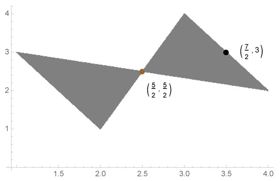
The corresponding NE payoffs are $\left({\Pi }_a(\frac{\pi }{2},\frac{\pi }{2},\frac{\pi }{2},0),{\Pi }_b(\frac{\pi }{2},\frac{\pi }{2},\frac{\pi }{2},0)\right)=(\frac{7}{2},3)$. They are higher than classical payoffs and lie on the Pareto frontier of classical mixed strategies [22] (see also Figure 1).

Figure 1. Payoff polygon for game (21) with the classical (brown) and quantum (black) equilibrium payoff vectors.

In this way, we get a truly quantized game with a non-trivial and Pareto efficient Nash equilibrium which is invariant with respect to isomorphic transformations of an input classical game.

Another property relates to $2\times 2$ bimatrix games for which there are dominant pairs of payoffs, i.e., pairs of strategies that guarantee both players the highest payoffs.

Proposition 2. 

Let us suppose that the bimatrix (1) has a dominant pair of payoffs—i.e., there exists $k,l\in \{0,1\}$ such that $p_{kl}={max}_{i,j}\left\{p_{ij}\right\}$ for $p\in \{a,b\}$. Then, the game (2) has Nash equillibria $\left({\theta }_a^{*},{\varphi }_a^{*},{\theta }_b^{*},{\varphi }_b^{*}\right)$ of the form

i. 

$(0,\varphi ,0,-\varphi )$ and $(\pi ,\varphi ,\pi ,\pi -\varphi )$ for $p_{00}={max}_{i,j}\left\{p_{ij}\right\}$,

ii. 

$(0,\varphi ,0,\pi -\varphi )$ and $(\pi ,\varphi ,\pi ,-\varphi )$ for $p_{11}={max}_{i,j}\left\{p_{ij}\right\}$,

iii. 

$(0,\varphi ,\pi ,\varphi )$ and $(\pi ,\varphi +\pi ,0,\varphi )$ for $p_{01}={max}_{i,j}\left\{p_{ij}\right\}$,

iv. 

$(0,\varphi +\pi ,\pi ,\varphi )$ and $(\pi ,\varphi ,0,\varphi )$ for $p_{10}={max}_{i,j}\left\{p_{ij}\right\}$,

v. 

$(0,\varphi ,0,{\varphi }^{\prime })$ and $(\pi ,\varphi ,\pi ,{\varphi }^{\prime })$ for $p_{00}=p_{11}={max}_{i,j}\left\{p_{ij}\right\}$,

vi. 

$(0,\varphi ,\pi ,{\varphi }^{\prime })$ and $(\pi ,\varphi ,0,{\varphi }^{\prime })$ for $p_{01}=p_{10}={max}_{i,j}\left\{p_{ij}\right\}$,

where $\varphi ,{\varphi }^{\prime }\in [0,2\pi )$. The payoffs at the Nash equilibria are equal to the dominant values ${\Pi }_p\left({\theta }_a^{*},{\varphi }_a^{*},{\theta }_b^{*},{\varphi }_b^{*}\right)=p_{kl}$.

Proof. 

The proof of this proposition can be derived directly from properties of payoff functions (6). In case i., let us assume that $({\theta }_a^{*},{\varphi }_a^{*},{\theta }_b^{*},{\varphi }_b^{*})=(0,\varphi ,0,-\varphi )$, for any $\varphi \in [0,2\pi )$. Notice that $P_{0,0}\left(0,\varphi ,0,-\varphi \right)=1$ and $P_{k,l}\left(0,\varphi ,0,-\varphi \right)=0$ for $(k,l)\ne (0,0)$. Therefore, for both $p=a,b$, we have

$${\Pi }_p(0,\varphi ,0,-\varphi )=\sum _{k,l=0}^1{P}_{k,l}(0,\varphi ,0,-\varphi )p_{kl}=p_{00}\ge {\Pi }_p({\theta }_a,{\varphi }_a,{\theta }_b,{\varphi }_b),$$

(23)

for arbitrary $({\theta }_a,{\varphi }_a,{\theta }_b,{\varphi }_b)\in D_a\times D_b$. The last inequality follows from the assumption that $p_{00}={max}_{i,j}\left\{p_{ij}\right\}$ and from normalization (8) of the payoffs coefficients. Thus, Equation (23) proves conditions (14) and (15) and yields the values of the NE payoffs at $p=a,b$. Similar inequalities hold for the second part of case i., where also $P_{0,0}\left(\pi ,\varphi ,\pi ,\pi -\varphi \right)=1$, which ends the proof of case i. The cases ii., iii. and iv., can be proven in a similar way. In the case v., let us notice that $P_{0,0}\left(0,\varphi ,0,{\varphi }^{\prime }\right)+P_{1,1}\left(0,\varphi ,0,{\varphi }^{\prime }\right)=1$ for any $\varphi ,{\varphi }^{\prime }\in [0,2\pi )$. Thus, for both $p=a,b$ we have

$${\Pi }_p(0,\varphi ,0,{\varphi }^{\prime })=\sum _{k,l=0}^1{P}_{k,l}(0,\varphi ,0,{\varphi }^{\prime })p_{kl}=p_{00}=p_{11}\ge {\Pi }_p({\theta }_a,{\varphi }_a,{\theta }_b,{\varphi }_b),$$

(24)

for arbitrary $({\theta }_a,{\varphi }_a,{\theta }_b,{\varphi }_b)\in D_a\times D_b$. An analogous inequality holds in the second part of the case v., because $P_{0,0}\left(\pi ,\varphi ,\pi ,{\varphi }^{\prime }\right)+P_{1,1}\left(\pi ,\varphi ,\pi ,{\varphi }^{\prime }\right)=1$. The last case can be proven analogously. □

Note that the 2-parameter set $D_p$ of players’ strategies (3) is a subset of the set $\mathsf{SU}(2)$ of all (3-parameter) unitary transformations. Therefore, it is clear from the above proof that the dominant pair of payoffs will also result in NE in the full $\mathsf{SU}(2)$ parameterization.

Example 2. 

Let us consider the game given by bimatrix

$$\begin{array}{cc}& \begin{array}{cc}q& 1-q\end{array}\\ \begin{array}{l}p\\ 1-p\end{array}& (\begin{array}{cc}(3,3)& (0,3)\\ (3,0)& (1,1)\end{array}),\end{array}$$

(25)

This game has two Nash equilibria in pure strategies $(p,q)=(0,0)$ and $(1,1)$ with the payoffs $(1,1)$ and $(3,3)$, respectively. It has a dominant pair of payoffs $p_{00}=(3,3)$; therefore, according to Proposition 2, it has also Nash equilibria for two pairs of strategies:

$$\left({\theta }_a^{*},{\varphi }_a^{*},{\theta }_b^{*},{\varphi }_b^{*}\right)=\left(0,\varphi ,0,-\varphi \right)\mathrm{and}\left(\pi ,\varphi ,\pi ,\pi -\varphi \right),\varphi \in [0,2\pi ).$$

(26)

The corresponding NE payoffs are equal to $(3,3)$. The payoff pair $(1,1)$ is not accessible within this type of quantum NE.

Propositions 1 and 2 provide sufficient conditions for the existence of Nash equilibria in the center ${\theta }_a^{*}={\theta }_b^{*}=\pi /2$ or at the boundary ${\theta }_a^{*},{\theta }_b^{*}\in \{0,\pi \}$ of $\theta$-parts of players’ strategy spaces $D_p$, respectively. It is also possible that the game has both types of NE. As an example, let us consider the matrix (21) from Example 1, in which the payoffs $a_{00}$ and $a_{10}$ are swapped. The resulting payoffs satisfy the assumptions of both propositions, and therefore, have both types of NE—the first defined in Proposition 1.ii. and the second defined in Proposition 2.iv. We speculate that within parameterization (3), Propositions 1 and 2 describe the only strategy profiles that allow for the existence of pure Nash equilibria.

4. Games without Pure Nash Equilibria

In this section, we will discuss classes of games in which there are no Nash equilibria in the strategy set (3). We begin our considerations by proving two technical lemmas concerning the scheme (2). They will be useful in proving the main statements of this section.

Lemma 1. 

For a fixed strategy $({\theta }_b^{*},{\varphi }_b^{*})$ of player b and a fixed strategy $({\theta }_a^{*},{\varphi }_a^{*})$ of player a, the following equations are satisfied:

$$\underset{{\theta }_a,{\varphi }_a}{max}(P_{0,0}({\theta }_a,{\varphi }_a,{\theta }_b^{*},{\varphi }_b^{*})+P_{i,j}({\theta }_a,{\varphi }_a,{\theta }_b^{*},{\varphi }_b^{*}))=1$$

(27)

and

$$\underset{{\theta }_b,{\varphi }_b}{max}(P_{0,0}({\theta }_a^{*},{\varphi }_a^{*},{\theta }_b,{\varphi }_b)+P_{i,j}({\theta }_a^{*},{\varphi }_a^{*},{\theta }_b,{\varphi }_b))=1.$$

(28)

for $(i,j)\in \{(0,1),(1,0)\}$.

Proof. 

As a first step, we prove (27) for $(i,j)=(1,0)$. Let us assume that ${\theta }_b^{*}\ne 0$ and ${\varphi }_b^{*}\ne {\varphi }_a-\pi$. Consider player a’s strategy $({\theta }_a,{\varphi }_a)$ that satisfies the following equations:

$$cot\frac{{\theta }_a}{2}=cot\frac{{\theta }_b^{*}}{2}tan\left(\frac{{\varphi }_a}{2}-\frac{{\varphi }_b^{*}}{2}\right),cos{\varphi }_a=cos(cos{\theta }_b^{*}cos{\varphi }_b^{*}).$$

(29)

Letting

$${\varphi }_a^{*}=arccos\left(cos{\theta }_b^{*}cos{\varphi }_b^{*}\right)$$

(30)

and

$${\theta }_a^{*}=2arccot\left(cot\frac{{\theta }_b^{*}}{2}tan\left(\frac{arccos\left(cos{\theta }_b^{*}cos{\varphi }_b^{*}\right)}{2}-\frac{{\varphi }_b^{*}}{2}\right)\right)$$

(31)

we conclude that

$$P_{0,0}({\theta }_a^{*},{\varphi }_a^{*},{\theta }_b^{*},{\varphi }_b^{*})+P_{1,0}({\theta }_a^{*},{\varphi }_a^{*},{\theta }_b^{*},{\varphi }_b^{*})=1.$$

(32)

For the case ${\theta }_b^{*}=0$ and ${\varphi }_b\in [0,2\pi )$, Equation (32) is satisfied when player a chooses $({\theta }_a^{*},{\varphi }_a^{*})=(0,-{\varphi }_b)$. Finally, for ${\varphi }_b^{*}={\varphi }_a^{*}-\pi$, Equation (30) implies ${\varphi }_a^{*}=\pi /2$, ${\varphi }_b^{*}=-\pi /2$. Then, Equation (32) holds true for ${\theta }_a^{*}=0$. To sum up, for any strategy of player b, player a can choose $({\theta }_a^{*},{\varphi }_a^{*})$ so that Equation (32) holds true. In the same manner, we prove Equation (27) for $(i,j)=(0,1)$. Let us first assume that

$$sin\frac{{\theta }_b}{2}sin\frac{{\varphi }_a-{\varphi }_b}{2}-cos\frac{{\theta }_b}{2}sin\frac{{\varphi }_a+{\varphi }_b}{2}\ne 0.$$

(33)

Consider a strategy $({\theta }_a^{*},{\varphi }_a^{*})$ such that

$${\varphi }_a^{*}=-arcsin(cos{\theta }_b^{*}sin{\varphi }_b^{*})$$

(34)

and

$${\theta }_a^{*}=-2arccot\left(\frac{cos\frac{{\theta }_b^{*}}{2}cos\frac{{\varphi }_a^{*}-{\varphi }_b^{*}}{2}+sin\frac{{\theta }_b^{*}}{2}cos\frac{{\varphi }_a^{*}+{\varphi }_b^{*}}{2}}{sin\frac{{\theta }_b^{*}}{2}sin\frac{{\varphi }_a^{*}-{\varphi }_b^{*}}{2}}\right).$$

Then

$$P_{0,0}({\theta }_a^{*},{\varphi }_a^{*},{\theta }_b^{*},{\varphi }_b^{*})+P_{0,1}({\theta }_a^{*},{\varphi }_a^{*},{\theta }_b^{*},{\varphi }_b^{*})=1.$$

(35)

If

$$sin\frac{{\theta }_b}{2}sin\frac{{\varphi }_a-{\varphi }_b}{2}=cos\frac{{\theta }_b}{2}sin\frac{{\varphi }_a+{\varphi }_b}{2}$$

(36)

then the expression $P_{1,0}({\theta }_a,{\varphi }_a,{\theta }_b,{\varphi }_b)+P_{1,1}({\theta }_a,{\varphi }_a,{\theta }_b,{\varphi }_b)$ can be written as

$$\begin{array}{c}{cos}^2\frac{{\theta }_b}{2}{\left(cos\frac{{\varphi }_a-{\varphi }_b}{2}sin\frac{{\theta }_a}{2}+cos\frac{{\theta }_a}{2}sin\frac{{\varphi }_a+{\varphi }_b}{2}\right)}^2\hfill \\ +{\left(cos\frac{{\varphi }_a+{\varphi }_b}{2}sin\frac{{\theta }_a}{2}sin\frac{{\theta }_b}{2}-sin\frac{{\varphi }_a+{\varphi }_b}{2}cos\frac{{\theta }_a}{2}cos\frac{{\theta }_b}{2}\right)}^2.\end{array}$$

(37)

Letting ${\theta }_a=0$ yields $P_{1,0}({\theta }_a,{\varphi }_a,{\theta }_b,{\varphi }_b)+P_{1,1}({\theta }_a,{\varphi }_a,{\theta }_b,{\varphi }_b)=0$. As a result, we obtain $P_{0,0}({\theta }_a,{\varphi }_a,{\theta }_b,{\varphi }_b)+P_{0,1}({\theta }_a,{\varphi }_a,{\theta }_b,{\varphi }_b)=1$. Similar arguments apply to Equation (28). □

Lemma 2. 

Let $({\theta }_a,{\varphi }_a,{\theta }_b,{\varphi }_b)$ be a strategy profile in (2), and $P_{i,j}({\theta }_a,{\varphi }_a,{\theta }_b,{\varphi }_b)$ is given by (6). If $P_{i,j}({\theta }_a,{\varphi }_a,{\theta }_b,{\varphi }_b)=1$ for some $i,j\in \{0,1\}$, then ${\theta }_a^{*}={\theta }_b^{*}\in \{0,\pi \}$.

Proof. 

There is no loss of generality in assuming $P_{0,0}({\theta }_a,{\varphi }_a,{\theta }_b,{\varphi }_b)=1$. Then, $P_{1,1}({\theta }_a,{\varphi }_a,$${\theta }_b,{\varphi }_b)=0$, and from (6) it follows that

$$\begin{array}{c}\hfill {\left(cos\frac{{\theta }_a}{2}cos\frac{{\theta }_b}{2}cos\left(\frac{{\varphi }_a+{\varphi }_b}{2}\right)+sin\frac{{\theta }_a}{2}sin\frac{{\theta }_b}{2}sin\left(\frac{{\varphi }_a+{\varphi }_b}{2}\right)\right)}^2=1,\\ \hfill {\left(cos\frac{{\theta }_a}{2}cos\frac{{\theta }_b}{2}sin\left(\frac{{\varphi }_a+{\varphi }_b}{2}\right)-sin\frac{{\theta }_a}{2}sin\frac{{\theta }_b}{2}cos\left(\frac{{\varphi }_a+{\varphi }_b}{2}\right)\right)}^2=0.\end{array}$$

(38)

By squaring and adding both sides of Equation (38), we obtain

$${cos}^2\frac{{\theta }_a}{2}{cos}^2\frac{{\theta }_b}{2}+{sin}^2\frac{{\theta }_a}{2}{sin}^2\frac{{\theta }_b}{2}=1$$

(39)

which is equivalent to

$${cos}^2\frac{{\theta }_a}{2}{sin}^2\frac{{\theta }_b}{2}+{sin}^2\frac{{\theta }_a}{2}{cos}^2\frac{{\theta }_b}{2}=0.$$

(40)

The last equation is satisfied only for ${\theta }_a^{*}={\theta }_b^{*}\in \{0,\pi \}$, as claimed. □

Let us consider a symmetric game of the type

$$\left(\begin{array}{cc}(\gamma ,\gamma )& (\beta ,\alpha )\\ (\alpha ,\beta )& (\delta ,\delta )\end{array}\right),\alpha >\gamma >\delta ,\alpha >\beta ,and(\gamma ,\gamma )\notin Conv\left(\left\{(\alpha ,\beta ),(\delta ,\delta ),(\beta ,\alpha )\right\}\right),$$

(41)

where $Conv\left(·\right)$ denotes the convex hull of the set of points.

Proposition 3. 

There are no pure Nash equilibria of the game (41) in parameterization (3).

Proof. 

Let us consider the payoff functions

$$\begin{array}{cc}\hfill {\Pi }_a({\theta }_a,{\varphi }_a,{\theta }_b,{\varphi }_b)& =\gamma P_{0,0}({\theta }_a,{\varphi }_a,{\theta }_b,{\varphi }_b)+\beta P_{0,1}({\theta }_a,{\varphi }_a,{\theta }_b,{\varphi }_b)+\alpha P_{1,0}({\theta }_a,{\varphi }_a,{\theta }_b,{\varphi }_b)+\delta P_{1,1}({\theta }_a,{\varphi }_a,{\theta }_b,{\varphi }_b),\hfill \end{array}$$

(42)

$$\begin{array}{cc}\hfill {\Pi }_b({\theta }_a,{\varphi }_a,{\theta }_b,{\varphi }_b)& =\gamma P_{0,0}({\theta }_a,{\varphi }_a,{\theta }_b,{\varphi }_b)+\alpha P_{0,1}({\theta }_a,{\varphi }_a,{\theta }_b,{\varphi }_b)+\beta P_{1,0}({\theta }_a,{\varphi }_a,{\theta }_b,{\varphi }_b)+\delta P_{1,1}({\theta }_a,{\varphi }_a,{\theta }_b,{\varphi }_b).\hfill \end{array}$$

(43)

Suppose that there exists a Nash equilibrium $({\theta }_a^{*},{\varphi }_a^{*},{\theta }_b^{*},{\varphi }_b^{*})$. By Lemma 1, we conclude that player a’s response $({\theta }_a^{*},{\varphi }_a^{*})$ to an equilibrium strategy $({\theta }_b^{*},{\varphi }_b^{*})$ of player b implies

$${\Pi }_a({\theta }_a^{*},{\varphi }_a^{*},{\theta }_b^{*},{\varphi }_b^{*})=\gamma P_{0,0}({\theta }_a^{*},{\varphi }_a^{*},{\theta }_b^{*},{\varphi }_b^{*})+\alpha P_{1,0}({\theta }_a^{*},{\varphi }_a^{*},{\theta }_b^{*},{\varphi }_b^{*})\ge \gamma .$$

(44)

Similarly, if $({\theta }_a^{*},{\varphi }_a^{*})$ is an equilibrium strategy of player a, we can see that

$${\Pi }_b({\theta }_a^{*},{\varphi }_a^{*},{\theta }_b^{*},{\varphi }_b^{*})=\gamma P_{0,0}({\theta }_a^{*},{\varphi }_a^{*},{\theta }_b^{*},{\varphi }_b^{*})+\alpha P_{0,1}({\theta }_a^{*},{\varphi }_a^{*},{\theta }_b^{*},{\varphi }_b^{*})\ge \gamma .$$

(45)

Inequalities (44) and (45) show that a Nash equilibrium for each player would give each player at least $\gamma$. Since $(\gamma ,\gamma )\notin Conv\left((\alpha ,\beta ),(\delta ,\delta ),(\beta ,\alpha )\right)$, a strict inequality of (44) or (45) would mean that the other player gets less than $\gamma$ in the equilibrium. Therefore, there is no Nash equilibrium that would give a payoff vector other than $(\gamma ,\gamma )$.

Suppose that there exists a Nash equilibrium $({\theta }_a^{*},{\varphi }_a^{*},{\theta }_b^{*},{\varphi }_b^{*})$ with the outcome $(\gamma ,\gamma )$. Thus, a strategy profile $(({\theta }_a^{*},{\varphi }_a^{*}),({\theta }_b^{*},{\varphi }_b^{*}))$ that generates the payoff $\gamma$ obeys the following condition:

$$P_{0,0}({\theta }_a^{*},{\varphi }_a^{*},{\theta }_b^{*},{\varphi }_b^{*})=1.$$

(46)

By Lemma 2, it follows that ${\theta }_a^{*}={\theta }_b^{*}\in \{0,\pi \}$. Without loss of generality, we can assume that ${\theta }_b^{*}=0$. However, then, player b obtains $\alpha$ by choosing $({\theta }_a,{\varphi }_a)=(\pi ,{\varphi }_b^{*})$; i.e.,

$${\Pi }_a(\pi ,{\varphi }_b^{*},0,{\varphi }_b^{*})=\alpha >\gamma ={\Pi }_a({\theta }_a^{*},{\varphi }_a^{*},{\theta }_b^{*},{\varphi }_b^{*}).$$

(47)

This contradicts our assumption that $({\theta }_a^{*},{\varphi }_a^{*},{\theta }_b^{*},{\varphi }_b^{*})$ is a Nash equilibrium. □

An immediate consequence of Proposition 3 is the following corollary.

Corollary 1. 

There are no pure Nash equilibria of the game

$$\left(\begin{array}{cc}(\gamma ,\gamma )& (\beta ,\alpha )\\ (\alpha ,\beta )& (\delta ,\delta )\end{array}\right),\alpha >\gamma >\delta >\beta ,2\gamma >\alpha +\beta .$$

(48)

The game (48) is a well known prisoner’s dilemma. The condition that $(\gamma ,\gamma )$ is beyond the convex hull of the remaining payoffs (41) is equivalent to the last inequality in (48). Note that it is enough to replace the first inequality $\alpha >\gamma$ with an equality $\alpha =\gamma$ for the game (48) to have a dominant pair of payoffs and Nash equilibria in pure strategies. Such a case is presented in Example 2, where $\alpha =3,\gamma =3,\delta =1,\beta =0$. The first inequality $\alpha >\gamma$ in Proposition 3 is therefore crucial for the non-existence of Nash equilibria. It is also worth noting that the assumptions of Proposition 3 cover a wider class of games than just the Prisoner’s Dilemma. Assuming that $\beta >\delta$ in (41), we get the next corollary.

Corollary 2. 

There are no pure Nash equilibria of the game

$$\left(\begin{array}{cc}(\gamma ,\gamma )& (\beta ,\alpha )\\ (\alpha ,\beta )& (\delta ,\delta )\end{array}\right),\alpha >\gamma >\beta >\delta ,2\gamma >\alpha +\beta .$$

(49)

The game (49) is a special case of the game of Chicken. Examples for both corollaries can be given if we assume that $\alpha =4$, $\gamma =3$, $\delta =1$ and $\beta =0$ (for the prisoner’s dilemma) or $\beta =1$ and $\delta =0$ (for the game of chicken).

Example 3. 

According to Corollaries 1 and 2, the following games do not have Nash equilibria in pure strategies.

$$\left(\begin{array}{cc}(3,3)& (0,4)\\ (4,0)& (1,1)\end{array}\right)(\mathrm{the}\mathrm{prisoner}\text{’}\mathrm{s}\mathrm{dilemma})\mathrm{and}\left(\begin{array}{cc}(3,3)& (1,4)\\ (4,1)& (0,0)\end{array}\right)(\mathrm{the}\mathrm{game}\mathrm{of}\mathrm{chicken}).$$

(50)

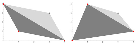
The payoff polygons of both games are shown in Figure 2. Here, one can also see the equivalence of conditions for $(\gamma ,\gamma )$ from Equations (41), (48) and (49), where gray payoffs are outside the convex hull of the set of red payoffs.

Figure 2. Payoff polygons for games (50).

In what follows, we examine another class of games that have no Nash equilibria. Let us now consider the following game.

$$\left(\begin{array}{cc}(\alpha ,\beta )& (\gamma ,\gamma )\\ (\gamma ,\gamma )& (\beta ,\alpha )\end{array}\right),\alpha >\beta ,(\alpha +\beta )/2>\gamma .$$

(51)

This game is more general than the battle of the sexes, for which $\alpha >\beta >\gamma$. For games of this type, the following proposition holds:

Proposition 4. 

There are no pure Nash equilibria of the game (51) in parameterization (3).

Proof. 

Using the expressions (11) and (10), the player’s $p=1,2$ payoff function of the game (51) is

$$\begin{array}{cc}\hfill {\Pi }_p\left({\theta }_a,{\varphi }_a,{\theta }_b,{\varphi }_b\right)=& \frac{\alpha +\beta }{4}(1+cos{\theta }_{a}cos{\theta }_b)+\frac{\gamma }{2}(1-cos{\theta }_{a}cos{\theta }_b)+\hfill \\ \hfill \pm & \frac{\beta -\alpha }{4}\left(cos({\varphi }_a+{\varphi }_b)(cos{\theta }_a+cos{\theta }_b)+sin({\varphi }_a+{\varphi }_b)sin{\theta }_{a}sin{\theta }_b\right),\hfill \end{array}$$

(52)

where “±” means “+” for player b and “−” for player a. Let us assume that the game has a Nash equilibrium at $({\theta }_a^{*},{\varphi }_a^{*},{\theta }_b^{*},{\varphi }_b^{*})$. The equilibrium is neither at $(0,{\varphi }_a^{*},\pi ,{\varphi }_b^{*})$ nor at $(\pi ,{\varphi }_a^{*},0,{\varphi }_b^{*})$ because according to (52) ${\Pi }_p\left(0,{\varphi }_a^{*},\pi ,{\varphi }_b^{*}\right)={\Pi }_p\left(\pi ,{\varphi }_a^{*},0,{\varphi }_b^{*}\right)=\gamma$, whereas there exist ${\varphi }_a$ such that ${\Pi }_p\left(0,{\varphi }_a,0,{\varphi }_b^{*}\right)\ge (\alpha +\beta )/2>\gamma$. We can therefore conclude that $({\theta }_a^{*},{\theta }_b^{*})\ne (0,\pi )$ and $({\theta }_a^{*},{\theta }_b^{*})\ne (\pi ,0)$. The second line in Formula (52) can be expressed by a single cosine function because

$$cos({\varphi }_a+{\varphi }_b)(cos{\theta }_a+cos{\theta }_b)+sin({\varphi }_a+{\varphi }_b)sin{\theta }_{a}sin{\theta }_b=Ccos({\varphi }_a+{\varphi }_b+\phi ),$$

(53)

where $C^2={(cos{\theta }_a+cos{\theta }_b)}^2+{sin}^2{\theta }_a{sin}^2{\theta }_b$. The phase $\phi =arctan\left(-\frac{sin{\theta }_{a}sin{\theta }_b}{cos{\theta }_a+cos{\theta }_b}\right)$ or $\phi =\pm \frac{\pi }{2}$ if $cos{\theta }_a+cos{\theta }_b=0$. Therefore, the payoff (52) can be transformed to a form in which it depends on ${\varphi }_a+{\varphi }_b$ only through one cosine function

$$\begin{array}{c}\hfill {\Pi }_p\left({\theta }_a,{\varphi }_a,{\theta }_b,{\varphi }_b\right)=\frac{\alpha +\beta }{4}(1+cos{\theta }_{a}cos{\theta }_b)+\frac{\gamma }{2}(1-cos{\theta }_{a}cos{\theta }_b)\pm \frac{\beta -\alpha }{4}Ccos({\varphi }_a+{\varphi }_b+\phi ).\end{array}$$

(54)

From the definition of NE, it follows that ${\Pi }_a\left({\theta }_a^{*},{\varphi }_a^{*},{\theta }_b^{*},{\varphi }_b^{*}\right)\ge {\Pi }_a\left({\theta }_a^{*},{\varphi }_a,{\theta }_b^{*},{\varphi }_b^{*}\right)$ for all ${\varphi }_a\in [0,2\pi )$. Note that equality holds only at ${\varphi }_a={\varphi }_a^{*}$. This is because the cosine in (54) reaches its maximum at only one point because $\alpha >\beta$ and $C\ne 0$ for $({\theta }_a^{*},{\theta }_b^{*})\ne (0,\pi )$ and $({\theta }_a^{*},{\theta }_b^{*})\ne (\pi ,0)$, as we assumed. Due to the sinusoidal term, ${\Pi }_a\left({\theta }_a^{*},{\varphi }_a,{\theta }_b^{*},{\varphi }_b^{*}\right)$ has its strict maximum at ${\varphi }_a={\varphi }_a^{*}$. However, at the same time, the payoff ${\Pi }_b\left({\theta }_a^{*},{\varphi }_a^{*},{\theta }_b^{*},{\varphi }_b\right)$ has its minimum at ${\varphi }_b={\varphi }_b^{*}$, because the last term of (54) has the opposite sign for player b. This shows that ${\Pi }_b\left({\theta }_a^{*},{\varphi }_a^{*},{\theta }_b^{*},{\varphi }_b^{*}\right)<{\Pi }_b\left({\theta }_a^{*},{\varphi }_a^{*},{\theta }_b^{*},{\varphi }_b\right)$ for some ${\varphi }_b$, and consequently, $({\theta }_a^{*},{\varphi }_a^{*},{\theta }_b^{*},{\varphi }_b^{*})$ is not a Nash equilibrium of (51). □

Note that the presented proof of Proposition 4 can be generalized to show the following corollaries.

Corollary 3. 

There are no pure Nash equilibria of the game

$$\left(\begin{array}{cc}(\alpha ,\beta )& ({\gamma }_1,{\gamma }_2)\\ ({\gamma }_1,{\gamma }_2)& (\beta ,\alpha )\end{array}\right),\alpha >\beta ,(\alpha +\beta )/2>{\gamma }_1,{\gamma }_2.$$

(55)

Using the symmetry of the payoff function with respect to the swapping of the second player strategies, one can prove also the next corollary.

Corollary 4. 

There are no pure Nash equilibria of the game

$$\left(\begin{array}{cc}({\gamma }_1,{\gamma }_2)& (\alpha ,\beta )\\ (\beta ,\alpha )& ({\gamma }_1,{\gamma }_2)\end{array}\right),\alpha >\beta ,(\alpha +\beta )/2>{\gamma }_1,{\gamma }_2.$$

(56)

5. Conclusions

In noncooperative quantum game theory, the dominant trend is to study games with respect to Nash equilibria. In our work, we focused on finding the equilibria in the specific 2-parameter set of unitary strategies. A quantum game with such strategies is invariant with respect to isomorphic transformation of the classical game, as the game with $\mathsf{SU}(2)$. Contrary to the special unitary group, there may be equilibria for these 2-parameter strategies in games for which players have different preferences regarding the final vector payoff. Our work was the first attempt to determine the form of Nash equilibria in the quantum approach to general $2\times 2$ bimatrix games in the assumed parameterization. We have formulated conditions for pure Nash equilibria that span large classes of games. By using the symmetrized form of the payoff function, we have shown in Proposition 1 that it is possible to find equilibria in the center (${\theta }_a^{*}={\theta }_b^{*}=\pi /2$) of the players’ strategy spaces. This leads to Nash equilibria in many games which do not have them in the strategy space $\mathsf{SU}(2)$. Proposition 2 summarizes the conditions for the existence of the equilibra in games with dominant pairs of payoffs. We identified a series of games that do not have Nash equilibria in the parametrization under study. In particular, these are the prisoner’s dilemma, some variants of the game of chicken and the battle of the sexes. Our considerations do not cover all types of games. We believe that the work is a good starting point to characterize the full topology of $2\times 2$ bimatrix games in terms of Nash equilibria.

References

- von Neumann, J. Zur Theorie der Gesellschaftsspiele. Math. Ann. 1928, 100, 295. [Google Scholar] [CrossRef]
- von Neumann, J.; Morgenstern, O. Theory of Games and Economic Behavior; Princeton University Press: Princeton, NJ, USA, 1944. [Google Scholar]
- Meyer, D.A. Quantum strategies. Phys. Rev. Lett. 1999, 82, 1052. [Google Scholar] [CrossRef]
- Eisert, J.; Wilkens, M.; Lewenstein, M. Quantum Games and Quantum Strategies. Phys. Rev. Lett. 1999, 83, 3077–3080. [Google Scholar] [CrossRef]
- Marinatto, L.; Weber, T. A quantum approach to static games of complete information. Phys. Lett. A 2000, 272, 291. [Google Scholar] [CrossRef]
- Li, H.; Du, J.; Massar, S. Continuous-variable quantum games. Phys. Lett. A 2002, 306, 73. [Google Scholar] [CrossRef]
- Khan, S.; Alam, S. The dynamics of Nash equilibrium under non-Markovian classical noise in quantum Prisoners’ Dilemma. Rep. Math. Phys. 2018, 81, 399–413. [Google Scholar] [CrossRef]
- Khan, F.S.; Bao, N. Quantum Prisoner’s Dilemma and high frequency trading on the quantum cloud. Front. Artif. Intell. 2021, 4, 769392. [Google Scholar] [CrossRef]
- Shi, L.; Xu, F. Quantum Stackelberg duopoly game with isoelastic demand function. Phys. Lett. A 2021, 385, 126956. [Google Scholar] [CrossRef]
- Iqbal, A.; Abbott, D. Two-player quantum games: When player strategies are via directional choices. Quantum Inf. Process. 2022, 21, 212. [Google Scholar] [CrossRef]
- Benjamin, S.C.; Hayden, P.M. Comment on “Quantum games and quantum strategies”. Phys. Rev. Lett. 2001, 87, 069801. [Google Scholar] [CrossRef]
- Szopa, M. How Quantum Prisoner’s Dilemma Can Support Negotiations. Optim. Stud. Ekon. 2014, 5, 90–102. [Google Scholar] [CrossRef]
- Frąckiewicz, P. Quantum games with unawareness. Entropy 2018, 20, 555. [Google Scholar] [CrossRef] [PubMed]
- Flitney, A.P.; Hollenberg, L.C.L. Nash equilibria in quantum games with generalized two-parameter strategies. Phys. Lett. A 2007, 363, 381. [Google Scholar] [CrossRef][Green Version]
- Du, J.; Xu, X.; Li, H.; Zhou, X.; Han, R. Playing Prisoner’s Dilemma with quantum rules. Fluct. Noise Lett. 2002, 2, R189. [Google Scholar] [CrossRef]
- Du, J.; Li, H.; Xu, X.; Shi, M.; Wu, J.; Zhou, X.; Han, R. Experimental realization of quantum games on a quantum computer. Phys. Rev. Lett. 2002, 88, 137902. [Google Scholar] [CrossRef] [PubMed]
- Chen, L.K.; Ang, H.; Kiang, D.; Kwek, L.C.; Lo, C.F. Quantum prisoner dilemma under decoherence. Phys. Lett. A 2003, 316, 317. [Google Scholar] [CrossRef]
- Li, Q.; Iqbal, A.; Chen, M.; Abbot, D. Quantum strategies win in a defector-dominated population. Physica A 2012, 391, 3316. [Google Scholar] [CrossRef]
- Nawaz, A. The strategic form of quantum Prisoners’ Dilemma. Chin. Phys. Lett. 2013, 30, 050302. [Google Scholar]
- Frąckiewicz, P. Strong isomorphism in Eisert-Wilkens-Lewenstein type quantum game. Adv. Math. Phys. 2016, 2016, 4180864. [Google Scholar] [CrossRef]
- Frąckiewicz, P.; Pykacz, J. Quantum games with strategies induced by basis change rules. Int. J. Theor. Phys. 2017, 56, 4017. [Google Scholar] [CrossRef]
- Szopa, M. Efficiency of Classical and Quantum Games Equilibria. Entropy 2021, 23, 506. [Google Scholar] [CrossRef] [PubMed]
Publisher’s Note: MDPI stays neutral with regard to jurisdictional claims in published maps and institutional affiliations. |
© 2022 by the authors. Licensee MDPI, Basel, Switzerland. This article is an open access article distributed under the terms and conditions of the Creative Commons Attribution (CC BY) license (https://creativecommons.org/licenses/by/4.0/).